Hybrid grid/basis set discretizations of the Schrödinger equation

Abstract

We present a new kind of basis function for discretizing the Schrödinger equation in electronic structure calculations, called a gausslet, which has wavelet-like features but is composed of a sum of Gaussians. Gausslets are placed on a grid and combine advantages of both grid and basis set approaches. They are orthogonal, infinitely smooth, symmetric, polynomially complete, and with a high degree of locality. Because they are formed from Gaussians, they are easily combined with traditional atom-centered Gaussian bases. We also introduce diagonal approximations which dramatically reduce the computational scaling of two-electron Coulomb terms in the Hamiltonian.

I Introduction

Most numerical simulations of the Schrödinger cannot work directly in the continuum; they require a discretization of some sort that maps the continuum to a finite number of degrees of freedom. For example, in the many thousands of electronic structure calculations performed annually for molecules and solids, basis sets are usually used. For molecules, these are usually atom centered functions composed of linear combinations of Gaussian type functions, for which analytic integrals are used to quickly generate the discrete Hamiltonian terms. For solids, plane wave basis sets are often used, which also have analytic integrals. These basis set methods have been developed and refined over most of a century, and the software to use them has been improved to a remarkable degree. Nevertheless, a variety of alternative discretization methods, such as wavelet basesHarrison et al. (2004); Yanai et al. (2015); Mohr et al. (2014) adapted gridsModine et al. (1997); Beck (2000), finite elementsWhite et al. (1989), and sinc-function basesJones et al. (2016) have continued to be developed. These alternatives have been pursued to address real weaknesses in existing discretizations, but Gaussian and plane wave bases are still used for most calculations.

What is the motivation to try to make an improved discretization approach again? Our primary reason is that some of the most promising new strong-correlation methods for electronic structure—the density matrix renormalization group (DMRG)White (1992); White and Martin (1999); Chan and Sharma (2011), and related tensor network methodsNakatani and Chan (2013)—depend strongly on the discretization. These methods have strong requirements for locality in the basis, due to the low-entanglement nature of their approximations. One can use localized Gaussian basis sets for DMRG, but this combination does not perform nearly as well as DMRG for simple lattice models, like the Hubbard model. The ideal basis for a DMRG or tensor network electronic structure calculation would be some sort of hypothetical real space grid with a very modest number of grid points, comparable to the number of functions in an atom-centered Gaussian basis, and giving comparable accuracy. None of the current approaches approximate this ideal.

Our approach has two key new elements. The first is a novel type of basis function, called a gausslet, related to the scaling functions of wavelet approaches, designed to live on a uniform grid. Several features of these functions are particularly nice for electronic structure, particularly that they are orthogonal, localized, smooth, symmetric, and composed of a sum of Gaussians. The second new element is a set of diagonal approximations for the Hamiltonian elements. In making a diagonal approximation for the two electron interaction, the number of terms (integrals) needed drops from $N^{4}$ to $N^{2}$, where $N$ is the number of basis functions. This reduction is not a large-$N$ asymptotic feature—it appears for any $N$ with no large coefficient in front of the $N^{2}$. These two features take us a substantial way towards the performance of the hypothetical very coarse but accurate real space grid.

The next section gives a more detailed overview of the problem and the approach. Section III discusses grids of Gaussians as bases, which have nearly ideal completeness properties but suffer from near linear dependence. Section IV discusses ternary wavelet transformations which are used in Section V to derive gausslets. Section VI presents diagonal approximations, and Section VII has conclusions and a discussion of further directions. Throughout we give numerical examples in 1D.

II Overview

Consider an arbitrary basis set approach. The Hamiltonian is an operator with the coefficients of the operator terms defined by integrals over the basis. By far the most complex part of the Hamiltonian is the two-electron Coulomb interaction operator, parameterized by a four dimensional array or tensor

$$V_{ijkl}=\int_{\mathbf{r}_{1}}\int_{\mathbf{r}_{2}}\frac{\phi_{i}(\mathbf{r}_{1})\phi_{l}(\mathbf{r}_{1})\phi_{j}(\mathbf{r}_{2})\phi_{k}(\mathbf{r}_{2})}{|\mathbf{r}_{1}-\mathbf{r}_{2}|}$$ (1)

where the $\phi_{i}(\mathbf{r})$ make up the set of $N$ basis functions, $i=1\ldots N$. In some simpler approximations (e.g. the local density approximation of density functional theory), one can bypass the use of $V_{ijkl}$ in favor of, say, solving the Poisson equation, but usually for more accurate methods treating electron-electron correlation explicitly, one cannot avoid dealing with $V_{ijkl}$, which has $N^{4}$ elements.

In contrast, a simple cubic grid discretization gives a representation of the electron-electron interaction which scales only as $N^{2}$, where now $N$ is the number of grid points. In such an approach, one could use finite-difference approximations to represent kinetic energy derivatives. The nucleus-electron and electron-electron interactions would be evaluated point-wise, with the two electron Hamiltonian terms taking the form $V_{ij}\hat{n}_{i}\hat{n}_{j}$, where $\hat{n}_{i}$ is the density operator on site $i$, and $V_{ij}=|\vec{r}_{i}-\vec{r}_{j}|^{-1}$ (with a suitable alteration at $i=j$).

Simple grids like this are rarely used for electronic structure because the $N$ for an accurate 3D grid would be much bigger than for a typical basis. Consider a single atom: the grid spacing needs to be set to resolve behavior near the nucleus, resulting in many grid points to describe the tails of the wavefunction far from the nucleus. In contrast, in a Gaussian basis the tails of the wavefunction can be described using just a few basis functions. For example, in an early effort using a uniform 3D grid, utilizing finite elements rather than finite differences, as many as $10^{5}$ grid points were needed for accurate results for the moleculeWhite et al. (1989). Much more efficient approaches use adapted grids, putting more points near the nucleiModine et al. (1997). Neverthless, the number of grid points tends to be in the 1000’s even for second row diatomic molecules. Wavelet bases are another approach with much of the locality of a grid, and with adaptable increased resolution near nuclei, but again the number of functions tends to be substantially larger than in Gaussian bases. These types of methods can be useful for density functional theory or Hartree Fock calculations, but they are impractical for typical wavefunction methods treating correlation accurately.

Grid-like methods have a fundamental advantage for use with DMRG and other recently developed tensor network methods: these methods are based on the low entanglement of ground states when expressed in a local real-space basis. The entanglement of ground states is governed by the area law Eisert et al. (2010); Hastings (2007), which is specific to localized real space bases. In a delocalized basis, a volume law of entanglement holds instead, requiring the number of states $m$ kept to grow exponentially for fixed accuracy. Thus DMRG greatly prefers a real-space local representation. In addition, the calculation time for DMRG depends strongly on the number of two-electron interaction terms, so the $N^{4}$ scaling of $V_{ijkl}$ is a major drawback. The standard DMRG approach for molecules in a Gaussian basis utilizes a standard basis localization method before DMRG is used. This localization is less than ideal, and except in certain treatments of long chains, all $N^{4}$ two electron terms are kept.

The very recently developed sliced basis DMRG approach (SBDMRG)Stoudenmire and White (2017) uses a finite-difference grid in one direction (the long direction in a chain) and 2D Gaussians for the transverse directions. For chain systems, the SBDMRG grid gives a reduction to $O(N^{2})$ two electron terms, where $N$ scales linear with the length. SBDMRG also utilizes a compression algorithm for the long range terms, yielding a $O(N)$ calculation time, and chains of up to 1000 hydrogen atoms have been studied in the strongly correlated stretched-bond regime. While arbitrary molecules can, in principle, be treated with SBDMRG, it is particularly suited for long chains, even more than standard QCDMRG. One motivation for this work is to find a good way to increase the grid spacing in SBDMRG without loss of accuracy, for faster and more efficient SBDMRG calculations. However, a more important motivation is to take advantages of locality in all three dimensions.

Here we present techniques which do take us closer to an ideal combination of grid and basis discretizations. Our approach is related to orthogonal wavelet bases. Wavelets have and continue to be used successfully in electronic structure calculations, but our goals are different from many existing uses. A conventional wavelet basis can be used in a way that has precise control over the accuracy, with systematically improvable accuracy, in, say, a density functional theory calculation.Harrison et al. (2004) These approaches make no use of standard Gaussian bases which give an excellent description of core electrons with a very small number of functions. Thus the price of the precise control of accuracy is a basis that may have more than 1000 functions for a small molecule, which is not practical for most beyond-HF correlation calculations.

Our interest is in these correlation calculations, where one is interested in accuracies only up to about 1 mH, and for which Gaussian basis set descriptions of cores are fine, at least for energy differences. Thus we consider approaches where we use wavelet techniques in a very restricted way, combining them with standard Gaussian basis sets. A key consideration in developing such an approach is the calculation of integrals. To make this easy, we construct functions similar to the scaling functions of wavelet transforms, but out of an equal-spaced array of identical-width Gaussians. The resulting functions, called gausslets have a number of significant advantages for electronic structure calculations.

Gausslets live on a uniform grid, with one function per grid point. They are defined in 1D, but in 2 or 3D, one simply takes products of the 1D functions. Gausslets are orthogonal and symmetric, and almost compact in both real and momentum space, in the same sense that Gaussians are. They have excellent completeness properties for representing smooth functions. All standard integrals have simple analytic forms, although one has to contract over the underlying Gaussians. A gausslet is shown in Fig. 1, together with seven of the Gaussians of which it is composed. A 1D gausslet basis would be composed of this function plus integer translations, and the whole basis can be scaled to a grid spacing $a$.

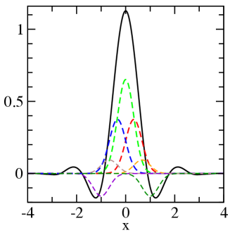
Figure 1: The gausslet ${\mathcal{G}}_{6}$ (solid line), along with some of the Gaussians of which it is composed, multiplied by their coefficients. A basis is formed by translating ${\mathcal{G}}_{6}$ to center it on every integer, and then scaling to any desired lattice spacing $a$ (here $a=1$). This basis is orthonormal and can represent any polynomial up to fourth order. Gausslets are exactly symmetric, and are defined as a sum of Gaussians of width $1/3$, with spacing $1/3$; ${\mathcal{G}}_{6}$ falls to about $10^{-12}$ at $x=\pm 12.5$.

Gausslets are constructed using a recently developed class of wavelet transforms which use a factor of three scaling transformation rather than the usual factor of two, in order to make them exactly symmetric. They have an additional very important property: they integrate like a $\delta$-function, for any low-order polynomial $p(x)$:

$$\int_{-\infty}^{\infty}dx\ {\mathcal{G}}(x-b)p(x)=p(b)$$ (2)

This, in turn translates to reducing the two electron integrals from $N^{4}$ to $N^{2}$, $V_{ijkl}\to\tilde{V}_{ij}$, provided the interaction is smooth. One way to make the interaction smooth would be to replace the Coulomb electron electron interaction with a two-electron pseudopotentialPrendergast et al. (2001).

The first step in constructing gausslets is understanding the properties of arrays of equally spaced, equal-width Gaussians.

III Arrays of Gaussians

Arrays of Gaussians with identical widths are particularly convenient to use in constructing basis functions because of their analytic integrals, their smoothness, their completeness, and also because the product space is greatly reduced and convenient. The product of a Gaussian of width $w$ located at $i$, and another of width $w$ at $j$, is a Gaussian centered at $(i+j)/2$ of width $w/\sqrt{2}$; the set of all products of a grid of $N$ such Gaussians is a half-spaced grid with roughly $2N$ functions, rather than $N^{2}$ functions. The product space plays a central role in defining Hamiltonian matrix elements, so this simplification can significantly improve computational efficiency.

The completeness properties of arrays of Gaussians are interesting. As is common in numerical analysis, we define completeness in terms of representing low order polynomials. A grid of basis functions with good polynomial completeness is excellent at representing arbitrary smooth functions. Consider a unit-spaced 1D grid, and on each integer point $j$ put a Gaussian with width $w$

$$g_{j}(x)\equiv\exp[-\frac{1}{2}\frac{(x-j)^{2}}{w^{2}}]$$ (3)

To see the completeness of the set $\{g_{j}\}$, consider the sum, shown in Fig. 2(a):

$$C(x)=\sum_{j}g_{j}(x).$$ (4)

Since the $g_{j}$ are identical except for translation, the representation within this basis of a constant function must be proportional to $C(x)$. If $C(x)$ is not nearly constant, the basis is very poor—it can’t even represent a constant.

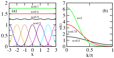
Figure 2: (a) An array of Gaussians and their sums, $C(x)$. (b) Overlap matrix eigenvalues.

We will show that $C(x)$ is very nearly constant for sufficiently large $w$. Note that $C$ is periodic, $C(x-1)=C(x)$, with period 1. Expand it in a Fourier series, with coefficients $c(k=2\pi n)$, where $n$ is an integer:

$$c(k) = \int_{0}^{1}dx\ C(x)\exp(-ikx)$$

$$= \sqrt{2\pi}w\exp(-\frac{1}{2}k^{2}w^{2}).$$

The largest deviation from constancy comes from the smallest nonzero $k$ in the series, namely $k=\pm 2\pi$, for which the factor $\exp(-\frac{1}{2}k^{2}w^{2})$ is $\exp(-2\pi^{2}w^{2})$. For $w=\sqrt{2}$, this factor is less than $10^{-17}$. For $w=1$, it is less than $10^{-8}$. Thus for modest width $w$, $C(x)$ is exactly constant to double precision accuracy (15 or 16 digits). In what follows, we choose $w=1$, since this lack of completeness at the $10^{-8}$ level appears in the wavefunction. According to standard variational arguments, it translates to errors in the energy of order $10^{-16}$. Note that higher terms in the series have much smaller coefficients, so that not only is $C(x)$ nearly constant, a number of higher derivatives are nearly zero. We will not try to make this particularly quantitative, since we can test any such property with a trivial numerical evaluation.

The flatness of $C(x)$—for the special case of Gaussians—also implies higher order polynomial completeness. In particular, we will show that the near constancy of $C(x)$ implies that, for $n\geq 1$, $\sum_{j}j^{n}g_{j}(x)$ is very nearly a polynomial in $x$ with order $n$. (We have already shown it is true for $n=0$.) If some linear combination of the $g_{j}$ can represent an order-$m$ polynomial for $0\leq m\leq n$, then one can find a suitable linear combination that can represent any polynomial up to order $n$. Gaussians have the property that their derivatives, to all orders, can be written as the same Gaussian times a polynomial. In particular, let $P(x,n)$ denote a polynomial in $x$ of degree $n$; the nth derivative of $g_{j}(x)$ can be written as

$$g_{j}^{(n)}(x) = P(x-j,n)g_{j}(x)$$

$$= \sum_{l,m}C_{l,m}j^{l}x^{m}g_{j}(x)$$

where $C_{l,m}=0$ if $l+m>n$. The nth derivative of $C(x)$ is

$$0\approx C^{(n)}(x)=\sum_{l,m}C_{l,m}x^{m}\sum_{j}j^{l}g_{j}(x).$$ (6)

In order to prove our result by induction, we pick out the $l=n$ term, for which $m=0$, and assume that for $l<n$, $\sum_{j}j^{l}g_{j}(x)$ is a polynomial $P_{l}(x)$. Then

$$C_{l,0}\sum_{j}j^{n}g_{j}(x)\approx-\sum_{l<n,m}C_{l,m}x^{m}P_{l}(x).$$ (7)

Since $C_{l,m}=0$ if $l+m>n$, this means that if $\sum_{j}j^{l}g_{j}(x)$ is very nearly an order-$l$ polynomial for all $l<n$, then it is an order $n$ polynomial for $l=n$. By induction, this is true for any $n$. This result breaks down when $C^{(n)}(x)$ stops being zero for large $n$. For $w\gtrsim 1$ , the breakdown does not occur very quickly, and an array of Gaussians has approximate polynomial completeness to high order.

The weakness of a grid of Gaussian as a basis is its lack of orthogonality, and that orthogonalizing the functions involves a fairly singular matrix, associated with a near lack of linear independence. Let $S(j,k)=S(j-k)=\langle g_{j}|g_{k}\rangle$ be the overlap matrix of the $\{g_{j}\}$. We can form an orthonormal set of functions (all related by integer translations) using $q(j-k)\equiv S^{-1/2}(j,k)$ as

$$G_{j}(x)\equiv\sum_{k}q(j-k)\ g_{k}(x).$$ (8)

However, $S$ becomes increasing singular as $w$ increases. The eigenvectors of $S$ are plane waves, and the most singular point is at momentum $\pi$; this corresponds to near cancellation of $g_{j}$. For example, for $w=\sqrt{2}$, the unnormalized fit to a momentum $\pi$ plane wave, $\sum_{j}(-1)^{j}g_{j}(x)$, is only of order $10^{-4}$ in magnitude. The near singularity of $S$ means that the $G_{j}$ have long tails and widely varying coefficients for the component Gaussians, making them computationally poorly behaved.

Fortunately the orthogonalization does not spoil the completeness, nor would a generic convolution of the form Eq. (8), transforming $g\to G$ using an arbitrary vector $q$. Consider

$$\sum_{j}P(j,n)G_{j}(x)=\sum_{k}\left[\sum_{j}q(j-k)P(j,n)\right]g_{k}(x).$$ (9)

The term in square brackets is a polynomial in $k$ of degree $n$, so the entire right side is a polynomial in $x$ of degree $n$. By the same reasoning as above, this implies that the $G_{j}$ have the same excellent completeness properties as the $g_{j}$.

In summary, a grid of Gaussians has excellent completeness, as well as several other very desirable features, but poor orthogonality and linear independence properties. Fortunately, as we show in the next two sections, these faults can be fixed using wavelet technology.

IV Ternary Wavelet Transformations

In conventional compact orthogonal wavelet theory, as pioneered largely by Daubechies,Daubechies (1992) it is not possible to have a symmetric, compact, orthogonal wavelet transformation (WT). However, with ternary WTs , which change scales by a factor of 3 instead of 2, symmetry, orthogonality, and compactness are compatible. Recently Evenbly and White (E&W)Evenbly and White (2016) introduced new families of ternary WTs with excellent completeness, compactness, and smoothness properties, which we will make use of and extend. A very carefully chosen set of coefficients $c_{k}$, $-m\leq k\leq m$, with $c_{-k}=c_{k}$, defines a symmetric wavelet transform. Given a single function $f(x)$, we define all integer translations $f_{j}(x)=f(x-j)$ to form a basis set that lives on an integer grid. Then the wavelet transform produces a new basis set, also living on a grid with unit spacing, defined by a function $f^{\prime}$, defined by

$$f^{\prime}(x)=\sum_{k}c_{k}f(3x-k)$$ (10)

The scaling function of the WT is the fixed point of Eq. (10). The fixed point exists provided the initial $f$ satisfies some simple conditions, most importantly that they sum to a constant (exactly), $\sum_{j}f_{j}(x)={\rm const}$. Thus any functions defined by Gaussians with finite $w$ are technically not suitable for generating the fixed point. However, if one only wants to apply the WT a modest number of times, Gaussian derived functions can be an excellent starting point. Since we do not plan to use the wavelets to represent sharp core functions (instead using standard Gaussians), a full multiscale resolution analysis is not needed, and for our uses, the fixed point is entirely unnecessary.

E&W showed that WTs have a direct correspondence with quantum circuit theory. The circuit corresponding to a WT is defined by a small number of angles $\theta_{k}$; each angle defines a unitary “gate”, which is a $2\times 2$ or $3\times 3$ unitary matrix. The unitarity of the circuit is independent of the values of $\theta_{k}$, removing an annoying set of constraints when optimizing a WT. The circuits express symmetry much more naturally than in conventional approaches. Some of the symmetric ternary WTs constructed by E&W appear to have better properties than any previous such WTs.

Besides the transformation of the scaling function in Eq. (10), the WT produces two wavelet functions per scaling function. The scaling function captures the lowest momenum behaviour, while the wavelets describe high momentum. These wavelets are less central to our discussion here.

In the terminology of E&W, we consider here only Type I site-centered symmetric ternary wavelets. These are characterized by the number of low and high frequency moments associated with the scaling functions. We make this more specific here with the notation $W_{nlh}$ to describe the WT with $n$ angles, $l$ low moments, and $h$ high moments. The number $n$ also gives the number of layers of the circuit, fixing the range of the $c_{k}$, specifically from $-(3n-2)$ to $3n-2$, with $c_{-k}=c_{k}$. The number $l$ gives the completeness of the scaling functions; more specifically, $l-1$ is the maximum polynomial order the scaling functions fit exactly, which is imposed by making the wavelets orthogonal to any $l$th degree polynomial. Similarly, $h$ controls the smoothness; specifically, $h-1$ gives the number of sign-flipped polynomials $(-1)^{k}k^{h}$ the scaling functions are orthogonal too, which also corresponds to the Fourier transform of the $c_{k}$ having vanishing value and $h-1$ derivatives at maximum momentum $\pi$.

A related and important property of the corresponding scaling functions is that they integrate polynomials like a $\delta$-function. This is associated with a property of the $c_{k}$:

$$\sum_{k}c_{k}k^{m}=\sqrt{3}\delta_{m,0}$$ (11)

for $m=0,\ldots,p-1$ for some $p$. (The evenness of the $c_{k}$ makes this statement trivial for odd $m$.) The $\delta$-function order $p$ is related to the other moments, but not in a simple way: we have found WTs with the same $n$, $l$, and $h$, but with different $p$. Usually, however, a large $p$ appears “for free” from optimizing $l$ and $h$.

E&W give just a few examples of these types of WTs, and not to full double precision. Determination of a $W_{nlh}$ involves a nontrivial nonlinear optimization; we have found $W_{nlh}$ to high precision both for the examples of E&W and a number of additional WTs with higher order. All useful WTs had even $n$, and it is difficult to converge useful WT for higher $n$. Angles for the most useful WTs are listed in Table I. These emphasize completeness over smoothness, but not completely, mostly setting $h=2$ (which is only one constraint, since the order-1 high moment is automatically satisfied because of symmetry). The scaling functions with $h=2$ are nicely smooth; for $h=0$ they are much more irregular. This leaves $n-1$ degrees of freedom for completeness, i.e. $l=n-1$. Below we construct gausslets out of $W_{432}$, $W_{652}$, $W_{872}$, and $W_{1092}$. These WTs all have impressively high $p$’s given by a simple formula: $p=2l$.

	xxx $W_{212}$ xxx	xxx $W_{220}$ xxx
$\theta_{1}$	0.16991845472706096855	0.27564279921626540397
$\theta_{2}$	0.78539816339744830962	0.67967381890824387419

	xxx $W_{432}$ xxx	xxx $W_{652}$ xxx
$\theta_{1}$	0.33591409249043635638	0.47808035535078662712
$\theta_{2}$	-1.46977679545346969482	0.61724603408318791423
$\theta_{3}$	-0.16599563776337538784	-1.39526939914470111011
$\theta_{4}$	2.25517495885091800443	-0.51453080478199670477
$\theta_{5}$	-	1.08710749852097545154
$\theta_{6}$	-	0.68268293409625710015

	xxx $W_{872}$ xxx	xxx $W_{1092}$ xxx
$\theta_{1}$	0.57548632554189299396	0.61183864100711914517
$\theta_{2}$	1.07092896697683457430	0.70680189527339659367
$\theta_{3}$	-0.53397048757827478700	-2.76090222438702891461
$\theta_{4}$	-0.84404057490329784656	0.82725175790860767489
$\theta_{5}$	-2.19779794769420972567	-0.63493786130732787550
$\theta_{6}$	-0.20902293951451481799	-0.23346217196976042571
$\theta_{7}$	2.32620056445765248695	1.21327891348912294041
$\theta_{8}$	0.76753271083842639987	-1.15390181597860903352
$\theta_{9}$	-	1.74064098592517567308
$\theta_{10}$	-	0.63870849816381350029

Table 1: Angles $\theta_{k}$ parameterizing wavelet transforms of various depths.

A WT can be applied to an array of Gaussians, producing a new basis where the functions are formed from sums of Gaussians. The completeness properties of the Gaussians are transfered by the WT to the new basis, up to the completeness order $l$. To see this, let $i$ index a grid with spacing 1, and $j$ (an integer) run over a grid with spacing $1/3$. Let $f_{i}(j)=c_{j-3i}$; we can think of $f_{i}$ as being a discrete basis function representing functions living on the $1/3$ grid. (Usually in wavelet theory one thinks of an infinite sequence of ever smaller grids, which represents the continuum in the limit of infinitesimal grid spacing. In contrast, we apply the WT to a grid of functions which are already continuous functions of $x$.) The WTs have a discrete completeness property that means we can write

$$j^{m}=\sum_{i}a_{i}f_{i}(j)$$ (12)

for $m<l$. Multiplying by $g_{j}(x)$ on both sides, and summing over $j$, we find that linear combinations

$$s_{i}(x)\equiv\sum_{j}f_{i}(j)g_{j}(x)$$ (13)

can represent arbitrary low order polynomials. Again, this implies that suitable linear combinations of the $s_{i}(x)$ can represent any low order polynomial. However, they are not orthogonal, which we address in the next section.

V Gausslets

We wish to use these properties of WTs and Gaussian grids to define convenient, orthogonal, complete functions defined as sums of Gaussians. There are several possible ways to proceed. One way starts with the $s_{i}(x)$. The $s_{i}(x)$ are not orthogonal, but their overlap matrix $S_{s}$ is much less singular than that of the $g_{j}(x)$. The $s_{i}(x)$ look like somewhat broadened wavelet scaling functions, with oscillations that partially cancel off-diagonal elements of the overlap matrix. (Further applications of a WT would take them closer to orthogonality.) One can use $S_{s}^{-1/2}$ to orthogonalize the $s_{i}$. The resulting functions are close to what we want, but $S_{s}^{-1/2}$ introduces moderately long tails in the final functions. One can then apply a WT to these orthogonal functions, which would substantially decrease the tails, and use those functions. The main drawback is that the underlying Gaussian grid would have a spacing of $1/9$ that of the final basis functions. The more Gaussians making up a basis function, the more computatonal work to use them, so we have developed a way to maintain the minimal $1/3$ spacing of the underlying Gaussians without the long tails.

It is possible to partially orthogonalize the $g_{j}(x)$, so that the application of a particular WT to the partially orthogonalized functions produces fully orthonormal functions. Let function $G_{j}(x)$ be defined by Eq. (8), for some vector $q(k)$, and then apply a WT (defined by $f_{i}(j)$):

$${\mathcal{G}}_{i}(x)\equiv\sum_{j}f_{i}(j)\ G_{j}(x).$$ (14)

We know that a $q(k)$ exists that makes the ${\mathcal{G}}_{i}(x)$ orthonormal—we can use the overlap matrix $S_{s}$ to make $q(k)$, which completely orthonormalizes the $G_{j}(x)$, and thus the ${\mathcal{G}}_{i}(x)$. In that case, $q(k)$ falls to about $10^{-12}$ near $k=110$, so it is rather nonlocal, making ${\mathcal{G}}_{i}$ have long tails. It is possible to find a much more compact $q(k)$ if it is optimized for a particular WT, requiring orthogonality only of the ${\mathcal{G}}_{i}$ and not both the $G_{j}$ and the ${\mathcal{G}}_{i}$. The $q$ convolution and the WT each take care of parts of the orthogonalization. A typical $q$ is show in Fig. 3. Finding such a $q$ is a rather tedious nonlinear optimization problem, with many local minima. We implemented this optimization using a Nelder Mead algorithm, using restarts and high precision to deal with local minima, with the minimizations sometimes taking several days, and only achieving approximate double-precision orthogonality. A final orthogonalization step was performed to make the functions orthogonal to very high precision, with minimal impact on locality, using the inverse square root of the overlap matrix. Fortunately, using these functions does not require that these optimizations be repeated; all one needs are the final coefficients of the Gaussians, and the properties of the functions are easily verified.

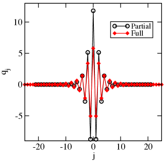
Figure 3: Full and partial orthogonalizing vectors $q(k)$, for the case of ${\mathcal{G}}_{6}$. The partial orthogonalizer extends out to $\pm 21$; the full orthogonalizer has fallen to about $10^{-12}$ at $j=110$.

This approach produces functions—gausslets—with a ratio of 3 between the spacing of the functions and the underlying Gaussians. Normally with WTs there is a tradeoff between order and compactness. The presence of the underlying Gaussians mean that there is an inherent limit to the size of a “$1/3$-gausslet” which is greater than the width of the fixed point scaling function of the WT used to make the gausslet. However, the gausslets are substantially smoother. We present coefficients for gausslets ${\mathcal{G}}_{4}$, ${\mathcal{G}}_{6}$, ${\mathcal{G}}_{8}$, and ${\mathcal{G}}_{10}$, where the index signifies $n$ of the underlying WT, $W_{n}$, which has $l=n-1$ and $h=2$. The gausslet ${\mathcal{G}}_{6}$ is shown in Fig. 1; the others look similar, with slightly increasing width with the order. The coefficients $b_{j}$ of these gausslets in terms of the underlying Gaussians are given in the Appendix in Table II-V.

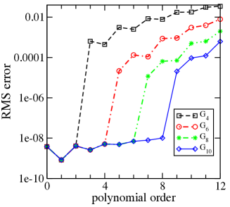
Figure 4: Root mean square errors in the fit of an array of gausslets with unit spacing to scaled Chebyshev polynomials $T_{n}(x/10)$, over the range $0\leq x\leq 1$, for gausslets of different orders, as a function of $n$. The gausslets of order $n$ are based on wavelet transformations designed to fit polynomials of order $0$ to $n-2$. The residual error of order $10^{-8}$ visible in the figure for small $n$ is due to the finite width and imperfect completeness of the underlying Gaussians making up the gausslets. Since the underlying Gaussians are the same for all the gausslets, the residual errors are approximately the same. The fitting errors of order $10^{-8}$ are expected to translate to energy errors of order $10^{-16}$.

A simple test of the completeness of the gausslets is shown in Fig. 4. The gausslets are fitted to polynomials of various orders and the root mean square errors over the unit interval are shown. (The gausslets involved in the fitting extend well outside this interval, because of the small but finite tails of the gausslets.) The fitting coefficients were approximated using the $\delta$-function property, as $T_{n}(i/10)$ for the gausslet centered at $i$, so this test of the fitting also tests the $\delta$-function property. Since the order of the $\delta$-function property is much higher than for fitting property, one sees only the errors associated with the fitting.

One may wish to have more compact gausslets, paying the price of an underlying finer array of Gaussians. Suitable $1/9$, $1/27$, etc. gausslets are easily derived by applying WTs to one of the ${\mathcal{G}}_{n}$. We label these gausslets as in the following example: ${\mathcal{G}}_{864}$ is formed from ${\mathcal{G}}_{8}$ and applying $W_{6}$ and then $W_{4}$. These constructions also generate useful wavelet-like functions, and a multiresolution basis can be formed for a modest range of scales, with each length scale having different functions. If one successively applies $W_{n}$, the range of the functions decreases, and the basis functions become close to the scaling function of $W_{n}$. Alternatively, one can successively decrease the order over several steps, which produces very localized functions functions which are still smooth with a finite size underlying Gaussian array. An example of this is shown in Fig. 5. A multiscale basis can be useful, but in many cases a better alternative that produces smaller bases is to add atom-centered Gaussian functions to the gausslet basis. The extra functions can be orthogonalized to the gausslets and themselves. A simple 1D example of this approach is given below.

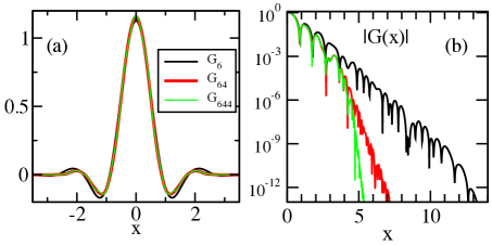
Figure 5: Comparison of a sequence of guasslets ${\mathcal{G}}_{6}$, ${\mathcal{G}}_{6}$₄, ${\mathcal{G}}_{6}$₄₄. Repeated application of a wavelet transform shrinks the tails of the functions.

As a first test of the use of gausslets to solve the Shrödinger equation, we apply them to two different simple 1D smooth potentials; see Fig. 6. The first, the Pöschl-Teller potential, is exactly solvable, with energy $E=-1/2$. The second, the soft Coulomb potential, has been used as a 1D model with properties such as correlation energies roughly similar to that of real 3D moleculesStoudenmire et al. (2012); Wagner et al. (2012). Here the SC potential would be that of pseudo-hydrogen. Each potential is centered at two positions to demonstrate that the grid points need not be aligned with the potential centers. To define the Hamiltonian matrices, we first evaluate the Hamiltonian matrix elements for the underlying Gaussian grid with spacing $a/3$, analytically for the kinetic energy, and numerically for the potentials. Then we transform to the gausslet basis using the $b_{j}$. Both of these potentials have widths of order 1, and we see that very high accuracy is easily achievable for $a\sim 0.2$. More important for our goals is that one achieves accuracies of $O(10^{-3})$ for $a\sim 1$. Large $a$ values are essential for applications to 3D.

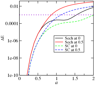
Figure 6: Energy errors in solving 1D potentials with a ${\mathcal{G}}_{10}$ gausslet basis with spacing $a$. Here the “Sech” potential is the exactly solvable Pöschl-Teller potential $V(x)=-{\rm sech}^{2}(x-b)$, for $b=0,0.5$, and the “SC” potential is the soft Coulomb potential $V(x)=-1/\sqrt{(x-b)^{2}+1}$, for $b=0,0.5$. The dotted line shows $\Delta E=10^{-3}$, a typical target accuracy for “chemically accurate” electronic structure calculations.

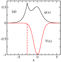
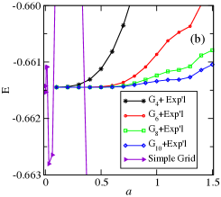
Figure 7: (a) A potential with a smooth part and a delta function, and the resulting ground state. (b) Convergence of the energy with grid spacing for two types of bases: 1) an array of gausslets plus an exponential which is the solution of the isolated delta function, for four different gausslets; and 2) a simple second order finite difference grid.

A key advantage of a basis set approach is that one can add functions to it to represent singularities or other sharp features. As a test of this, shown in Fig. 7 we consider a potential with a smooth part plus an off-center delta function, $V(x)=-\exp(-\frac{1}{2}x^{2})-\delta(x-2.7)$. Particularly in three dimensions, this sort of potential is difficult with a grid. Our basis consists of an array of gausslets plus, to represent the singularity, the solution to the delta function alone, $\exp(-|x-2.7|)$. The exponential is orthogonalized to the gausslets to make a fully orthogonal basis. To carry out the calculations, the exponential is first represented very accurately as a sum of a few hundred Guassians, the coefficients coming from a discretization of an integral. (In a 3D calculation, to describe, say, a 1S function, one would use a sum of a few Gaussians from a standard basis set.) Then all the potential terms are sums of analytic Gaussian integrals. The hybrid Gaussian/exponential approach converges very rapidly, with errors below about $10^{-3}$ for $a<1.5$ with ${\mathcal{G}}_{8}$ and ${\mathcal{G}}_{10}$. The energies for the last two points, $a=0.1$ and $a=0.2$, agree to eight digits, $E=-0.66144716$. For comparison, we implemented a naive grid, without trying to put a grid point exactly on the singularity. The grid results show substantial oscillations as a function of $a$. The finest grid result, $a=10^{-4}$, gives $E\approx-0.6614$, in agreement with the gausslet result but much less accurate.

VI Diagonal Approximations

A crucial feature of finite difference grid approximations is the simple form of the two electron interaction, $V_{ij}\hat{n}_{i}\hat{n}_{j}$. A similar property holds for the one electron nucleus-electron potential terms, which have the simple form $U_{i}\hat{n}_{i}$. This latter property is not so important in itself, since the extra computation time to deal with a $U_{ij}$ form of the potential is minor, but it does serve another useful purpose: approximations which make $U$ diagonal should generally do the same for $V$, since the two electron interaction acts on one electron with a single-particle potential determined by the locations of all the other electrons. We will consider the simpler single particle potential first, in one dimension. Diagonal representations such as these are a key property of bases made from the sinc functionJones et al. (2016). Here we find similar approximations for gausslets, implying that the high nonlocality of the sinc is not needed for this sort of approximation. Although we focus on the gausslets, similar approximations would work for the ternary wavelet scaling functions, and for certain types of traditional wavelet scaling functions with the $\delta$-function property, particularly coifletsDaubechies (1992).

Let $U(x)$ act on a continuum wavefunction $\psi(x)$ to give another wavefunction $\phi(x)$: $\phi(x)=U(x)\psi(x)$. We are interested in the coefficient of $\phi$ for basis function ${\mathcal{G}}_{i}$, written using the expansion of $\psi$ in terms of the ${\mathcal{G}}_{j}$:

$$\phi_{i}=\int dx\ {\mathcal{G}}_{i}(x)\phi(x)=\sum_{j}\psi_{j}\int dx\ {\mathcal{G}}_{i}(x)U(x){\mathcal{G}}_{j}(x).$$ (15)

This is the conventional non-diagonal form, with the last integral defining $U_{ij}$. Now assume that each ${\mathcal{G}}_{i}$ integrates like a weighted delta function, with location $x_{i}$:

$$\int dx\ {\mathcal{G}}_{i}(x)f(x)=f(x_{i})w_{i}$$ (16)

for any smooth function $f(x)$, with

$$w_{i}\equiv\int dx\ {\mathcal{G}}_{i}(x).$$ (17)

Then

$$\phi_{i}=\phi(x_{i})w_{i}=U(x_{i})\psi(x_{i})w_{i}=U(x_{i})\psi_{i}.$$ (18)

Thus we have a diagonal “point” approximation for $U$:

$$U_{ij}\to\delta_{ij}U(x_{i}).$$ (19)

Note that the locality of the gausslets means that $U_{ij}$ is small for $i$ far from $j$, but the diagonal approximation does not rely on this. In particular, we disregard the near-neighbor $j=i\pm 1$ terms even though they are not small.

There are two other closely related diagonal approximations. First, if the $\delta$-function property is only approximate, we may prefer to replace $U(x_{i})$ with its overlap with ${\mathcal{G}}_{i}$:

$$U_{ij}\to\delta_{ij}\int dx\ {\mathcal{G}}_{i}(x)U(x)/w_{i}.$$ (20)

One might hope that this “integral” approximation could be more accurate, since it averages the potential over a finite range, but one needs tests to see if it actually is an improvement. Second, let us assume that the $\{{\mathcal{G}}_{i}\}$ can exactly represent a constant function over the range of interest. Then $w_{k}$ is then the expansion coefficient for ${\mathcal{G}}_{k}$ to represent the identity function, and

$$1=\sum_{k}w_{k}{\mathcal{G}}_{k}(x).$$ (21)

Inserting this into Eq. (20) gives the “summed” approximation

$$U_{ij}\to\delta_{ij}\sum_{k}U_{ik}w_{k}/w_{i}.$$ (22)

For the special case where the ${\mathcal{G}}_{i}$ are a uniform grid of gausslets, $w_{k}=w_{i}$, and as the grid spacing goes to zero, smooth functions have $\psi_{k}\approx\psi_{i}$ in the close vicinity of a point $i$. In this case, $\sum_{k}U_{ik}\psi_{k}\approx\psi_{i}\sum_{k}U_{ik}$, providing another rough justification for Eq. (22). (This idea was the original inspiration for these diagonal approximations.)

Tests of the diagonal approximations are shown for the soft Coulomb potential in Fig. 8. One sees that all of the diagonal approximations become very precise for small $a$. In fact, although one cannot see it in this figure, the diagonal approximation curves and the non-diagonal full matrix curve come together faster as a function of $a$ than any of the curves converge to the exact result. This is because the $\delta$-function property paramenter $p$ is twice that of the completeness parameter $l$. This means that at small $a$, there is no point in using the full matrix–the result might not be exact, but the diagonal approximation doesn’t contribute significantly to any error. At larger $a$, the diagonal approximations introduce significant errors. The integral approximation (or equivalently for this case, the summed approximation) is significantly better than the point approximation.

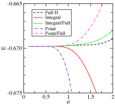
Figure 8: Energy solving the soft Coulomb potential (with $b=0$) using diagonal approximations with the ${\mathcal{G}}_{10}$ gausslet basis, as a function of spacing $a$. The “Full” curve uses the full Hamiltonian matrix. The “Integral” diagonal approximation is shown, which for these bases is identical to the “Summed” approximation. For the two diagonal approximations, we also show the energy evaluated with the full Hamiltonian, but with the eigenvector from the corresponding approximation.

These three approximations translate immediately into two electron approximations for $V$. The pointwise evaluation is

$$V_{ijkl}\to\delta_{il}\delta_{jk}V(x_{i},x_{j}).$$ (23)

The integral approximation replaces $V(x_{i},x_{j})$ in Eq. (23) with

$$V(x_{i},x_{j})\to\int dx\ dx^{\prime}\ {\mathcal{G}}_{i}(x)V(x,x^{\prime}){\mathcal{G}}_{j}(x^{\prime})/(w_{i}w_{j}).$$ (24)

The summed approximation replaces $V(x_{i},x_{j})$ with

$$V(x_{i},x_{j})\to\sum_{kl}V_{ijkl}w_{l}w_{k}/(w_{i}w_{j})$$ (25)

Because of the big difference in computational scaling associated with two electron versus one electron terms, it is sensible to only make the diagonal approximation for the two electron terms, using the full matrices for the one electron terms.

As a simple interacting example calculation we perform an exact diagonalization for a 1D helium atom in a soft Coulomb potential, with a basis of gausslets ranging from $-L$ to $L$. The results are shown in Fig. 9. According to Ref. Wagner et al. (2012), the exact energy from a grid DMRG calculation is -2.238. The two Full/Integral curves, which completely overlap, demonstrate that $L=7$ gives excellent convergence in $L$. All the diagonal approximations perform excellently at smaller $a$. For larger $a$ they still behave well; the Full/Integral approximation stays within 1 mH almost up to $a=1$. The point diagonal approximations are somewhat less accurate at larger $a$, but the Point/Point approximation is especially convenient for small $a$, since it is as accurate as the other approximations and requires no integral evaluations at all. For this case we went to $a=0.1$ and $L=15$, which gave 601 basis functions, to push for very high accuracy; we obtain $E=-2.238257824$, which we believe is correct to all the digits shown. The setup and diagonalization took less than 5 minutes on a desktop. With DMRG, it would be straightforward to extend these calculations to long chains.

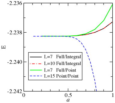
Figure 9: Energy solving the soft Coulomb 1D helium atom using gausslet basis ${\mathcal{G}}_{10}$ with diagonal approximations, as a function of spacing $a$. The approximations are labeled in the form (single particle approximation)/(two particle approximation). The lattice of gausslets extends approximately from $-L$ to $L$.

One can consider making the diagonal approximations after first making a mean-field-like reduction of the operator. For the one electron case derived below, this gives an energy correction but does not change the Hamiltonian. For the two electron terms, this produces altered one electron terms which change the diagonalization and might improve the results. For the one electron case, assume we have some estimate for $\langle\hat{c}^{\dagger}_{i}\hat{c}_{j}\rangle$, and let

$$\hat{U} = \sum_{ij}U_{ij}\hat{c}^{\dagger}_{i}\hat{c}_{j}$$ (26)

$$= \sum_{ij}U_{ij}(\hat{c}^{\dagger}_{i}\hat{c}_{j}-\langle\hat{c}^{\dagger}_{i}\hat{c}_{j}\rangle)+\sum_{ij}U_{ij}\langle\hat{c}^{\dagger}_{i}\hat{c}_{j}\rangle.$$ (27)

If we now apply a diagonal approximation $U_{ij}\to\tilde{U}_{ii}$ on the first term, we have

$$\hat{U}\approx\sum_{i}\tilde{U}_{ii}\hat{c}^{\dagger}_{i}\hat{c}_{i}+\left(\sum_{ij}U_{ij}\langle\hat{c}^{\dagger}_{i}\hat{c}_{j}\rangle-\sum_{i}\tilde{U}_{ii}\langle\hat{n}_{i}\rangle\right).$$ (28)

Suppose we use as our approximate $\langle\hat{c}^{\dagger}_{i}\hat{c}_{j}\rangle$ (and $\langle\hat{n}_{i}\rangle$) the result from the ground state using $\tilde{U}$. Then adding the correction term in the parentheses in Eq. (28) is the same as evaluating the energy in the full Hamiltonian of the eigenstate from the approximate Hamiltonian. This corrected result is shown in Fig. 8. We see that the corrected result is significantly better than the uncorrected result at large $a$. We leave exploring these mean-field approximations for the two electron term for future work.

A basis permitting a good diagonal approximation is special, and an orthogonal transformation of the basis will, in general, spoil the approximation. A truncation of the basis may not harm the approximation; in particular, a reduction of a particular set of orbitals into one orbital which is a linear combination from the set still allows a diagonal approximation. This is because a basis rotation takes two particle fermion number-conserving operators (i.e. $\hat{c}^{\dagger}_{i}\hat{c}_{j}$ or $\hat{n}_{i}$) into similar two particle operators, and a single orbital only has one such operator, $\hat{n}_{i}$. This applies also to the two-electron terms. If one knows the single particle reduced density matrix (RDM, $\langle\hat{c}^{\dagger}_{i}\hat{c}_{j}\rangle$), one can determine if reducing a particular set of functions to one function is a good approximation: it corresponds to the diagonal block over the sites of the RDM having just one significant eigenvalue. If so, that eigenvector would be the correct linear combination. One may expect that the outer tail regions of a molecule would satisfy this criterion, since far from the nuclei, the wavefunction decays in a simple way. This suggests that one should combine sites in the tail regions into tail functions, which could lead to a large reduction in the number of basis functions. If one transforms a set of basis function into a few functions, this breaks the diagonal approximation, but it only generates a limited number of off-diagonal terms, which may be acceptable. Specifically, if basis function $i$ is in the reduced set and $p$, $q$, and $r$ are outside the set, terms such as $\hat{c}^{\dagger}_{i}\hat{c}^{\dagger}_{p}c_{q}c_{r}$) with only one (or three) operators in the set are not generated.

A very important question is how to make a diagonal or near-diagonal approximation with a basis composed of an array of gausslets with some additional non-gausslet functions, particularly to represent the sharp behaviour near nuclei. We leave this question for future studies.

VII Discussion

Application of these ideas to sliced basis DMRG would require little development beyond what is presented here. The initial applications of SBDMRG used a finite difference grid which was adapted with a low-frequency filtering procedure to increase convergence with the grid spacing. Usually a grid spacing of 0.1 Bohr was used for hydrogen chains. The grid plus filtering procedure could be replaced by a gausslet basis, with a diagonal approximation introduced for the two-electron interaction. Probably this would allow substantially higher lattice spacing, and it would smooth the way for including larger $Z$ atoms.

More generally, for realistic 3D systems, one can form a 3D gausslet basis by making products of 1D gausslets, namely

$${\mathcal{G}}(x,y,z)={\mathcal{G}}(x){\mathcal{G}}(y){\mathcal{G}}(z)$$ (29)

If one is not worried about making diagonal approximations, then one can combine gausslets with 3D Gaussians from a standard Gaussian basis, orthogonalizing them to the gausslets. The fact that gausslets are made of Gaussians would facilitate this. Note that for a uniform grid of gausslets, all the two electron integrals between gausslets only need be done only once, and would be applicable to all systems, with a simple rescaling for different lattice spacings.

Diagonal approximation can be extremely effective in speeding up calculations, and so one would want to try to find approaches that allow them. The most straightforward approach would involve using a pseudopotential both of the usual one-electron type, and also a two-electron pseudopotentialPrendergast et al. (2001). This one electron pseudopotential means that a gausslet 3D grid, without supplementary Gaussians, would be adequate, and the two electron pseudopotental would allow any of our diagonal approximationn for the two electron interaction. The two-electron diagonal approximation would greatly speed up DMRG, and also allow other tensor network methods, such as projected entangled pair states (PEPS) to be tried. The diagonal interaction could be compressed for use in DMRG, just as is done in SBDMRG. The diagonal approximation may also speed up other correlation methods. To our knowledge, the combination of both types of pseudopotentials has not been used before, but it seems reasonably straightforward. The key question would be: what grid spacing is needed for reasonable accuracy?

For all electron calculations combining gausslets and 3D Gaussians, two-electron diagonal approximations would need to be tested and developed, since the extra functions do not fit within the $\delta$-function framework we used to derive diagonal approximations. Nevertheless, one might find approximations with acceptable accuracy. One could also consider whether diagonal approximations could be useful even in a standard Gaussian basis which has been localized by a standard method. Recently, Baker, Burke, and WhiteBaker et al. (2017) have proposed “wavelet localization” (WL), where an auxiliary wavelet basis is used to localize an existing delocalized basis, at the cost of a modest increase in the number of functions in the basis. One could equally use gausslets to perform wavelet localization. One scheme would be to WL to localize standard Gaussian atom-centered basis functions on each atom. The result would be functions which look standard Gaussians close to their nucleus, but midway to the next atom they would rapidly die off with oscillations to make them orthogonal to all functions on neighboring atoms. This might give rise to a modified diagonal approximation in which $V_{ijkl}$ is nonzero only if $i$ and $l$ are on the same atom, and $j$ and $k$ are on the same atom.

In conclusion, we have introduced gausslets, a new type of basis function, which combine the efficiencies of working with Gaussians, but with systematic completeness and orthogonality, while maintaining locality, symmetry, and smoothness. We have introduced diagonal approximations, which are tied to gausslets, which dramatically improve the scaling of electronic structure calculations, making them act more like a grid than a basis. Although the various tests we have performed here are in 1D, these basis functions were developed with 3D applications in mind, and we anticipate rapid development of 3D uses.

We thank Miles Stoudenmire, Glen Evenbly, Kieron Burke, Takeshi Yanai, Tom Baker, and Garnet Chan for helpful conversations. We acknowledge support from the Simons Foundation through the Many-Electron Collaboration, and from the U.S. Department of Energy, Office of Science, Basic Energy Sciences under award #DE-SC008696.

VIII Appendix: Coefficients of wavelets and gausslets

Here we give coefficients for the wavelets and gausslets described here. First, we present the coefficients of the gausslets, which are defined by

$${\mathcal{G}}(x)=\sum_{j}b_{j}\exp[-\frac{1}{2}(3x-j)^{2}]$$ (30)

The $b_{j}$ for gausslets with even order 4 through 10 are given in Tables II-V.

In Tables VI-XI, the coefficients defining ternary wavelet transforms are given. These can be used to define sequence of gausslets based on the primary gausslets given in Tables II-V. For example, applying a WT to a primary gausslet gives a gausslet with Gaussian spacing of $1/9$. Combining Eqs. (30) and (10), we have

$${\mathcal{G}^{\prime}}(x)=\sum_{l}\exp[-\frac{1}{2}(9x-l)^{2}]\sum_{k}c_{k}b_{l-3k},$$ (31)

where the $b_{j}$ come from the primary gausslet and the $c_{k}$ are the coefficients associated with the additional WT. To define wavelet-like functions coming from this transformation, we use the same formula, but with the mid or high wavelet coefficients replacing the $c_{k}$. One can repeat these WTs to construct a multi-level wavelet-like basis, where the functions at each scale, in addition to different scalings, are slightly different. All the basis functions in the multi-level basis would be written in terms a single grid of Gaussians, which would have a spacing a factor of three smaller than the finest level of wavelet-like functions.

$j$	$b_{j}$	$j$	$b_{j}$	$j$	$b_{j}$	$j$	$b_{j}$
$0$	$0.6067686239029718$	$12$	$-0.0007634581491839$	$24$	$-0.0000000111857638$	$36$	$-0.0000000000000001$
$1$	$0.4595762731397992$	$13$	$0.0001654718546793$	$25$	$0.0000000057570184$	$37$	$0.0000000000000000$
$2$	$-0.0164427190204405$	$14$	$-0.0001062974603036$	$26$	$0.0000000017544093$	$38$	$0.0000000000000003$
$3$	$-0.1403618655345050$	$15$	$0.0001489730491976$	$27$	$-0.0000000078396493$	$39$	$0.0000000000000004$
$4$	$-0.0402939401786279$	$16$	$-0.0000925527267679$	$28$	$0.0000000029209953$	$40$	$0.0000000000000003$
$5$	$0.0091345923715139$	$17$	$0.0000589148129012$	$29$	$-0.0000000011159594$	$41$	$-0.0000000000000004$
$6$	$0.0412074716875908$	$18$	$-0.0000343962098581$	$30$	$0.0000000006646346$	$42$	$-0.0000000000000005$
$7$	$-0.0263104231001814$	$19$	$0.0000139465804941$	$31$	$-0.0000000001080798$	$43$	$-0.0000000000000004$
$8$	$0.0120390822107673$	$20$	$-0.0000055900603412$	$32$	$-0.0000000000000000$	$44$	$-0.0000000000000001$
$9$	$-0.0041120776084794$	$21$	$0.0000021993752470$	$33$	$-0.0000000000000000$	$45$	$-0.0000000000000001$
$10$	$0.0003155814182348$	$22$	$-0.0000007773157565$	$34$	$-0.0000000000000000$	$46$	$-0.0000000000000001$
$11$	$0.0008905265359326$	$23$	$0.0000001821311458$	$35$	$0.0000000000000000$	$47$	$0.0000000000000000$
$12$	$-0.0007634581491839$	$24$	$-0.0000000111857638$	$36$	$-0.0000000000000001$	$48$	$0.0000000000000001$

Table 2: Coefficients $b_{j}$ of the Gaussians defining the gausslet ${\mathcal{G}}_{4}$ for $j\geq 0$, where $b_{-j}=b_{j}$.

$j$	$b_{j}$	$j$	$b_{j}$	$j$	$b_{j}$	$j$	$b_{j}$
$0$	$0.6510799122138565$	$10$	$-0.0129995132051085$	$20$	$0.0000527579539840$	$30$	$0.0000000012233441$
$1$	$0.3748901951337270$	$11$	$0.0083444621145336$	$21$	$-0.0000284802656230$	$31$	$0.0000000063863555$
$2$	$0.0939399437214329$	$12$	$-0.0035602045266604$	$22$	$0.0000150015015272$	$32$	$-0.0000000030684215$
$3$	$-0.1569006465627569$	$13$	$0.0012544959501549$	$23$	$-0.0000068808321161$	$33$	$0.0000000004500457$
$4$	$-0.0948155527751206$	$14$	$0.0003594627655807$	$24$	$0.0000028004555091$	$34$	$-0.0000000002218040$
$5$	$0.0232646256086860$	$15$	$-0.0007848423809006$	$25$	$-0.0000013067346743$	$35$	$0.0000000000913882$
$6$	$0.0216613768304792$	$16$	$0.0005747148102592$	$26$	$0.0000007168554123$	$36$	$0.0000000000104569$
$7$	$0.0361805021062946$	$17$	$-0.0003070053297971$	$27$	$-0.0000003912054599$	$37$	$-0.0000000000043992$
$8$	$-0.0317148981502408$	$18$	$0.0001499886588480$	$28$	$0.0000001613546686$	$38$	$-0.0000000000000000$
$9$	$0.0133915814065059$	$19$	$-0.0000895654658735$	$29$	$-0.0000000401650166$	$39$	$-0.0000000000000000$
$10$	$-0.0129995132051085$	$20$	$0.0000527579539840$	$30$	$0.0000000012233441$	$40$	$-0.0000000000000000$

Table 3: Coefficients of the Gaussians defining the gausslet ${\mathcal{G}}_{6}$.

$j$	$b_{j}$	$j$	$b_{j}$	$j$	$b_{j}$	$j$	$b_{j}$
$0$	$0.6188489361270065$	$12$	$-0.0046547275254753$	$24$	$0.0000289020341125$	$36$	$0.0000000067016738$
$1$	$0.3824167454273702$	$13$	$0.0040100201083541$	$25$	$-0.0000168829682435$	$37$	$-0.0000000032075046$
$2$	$0.1099474897465580$	$14$	$-0.0015184700034549$	$26$	$0.0000097119084642$	$38$	$0.0000000009153639$
$3$	$-0.1478654707279702$	$15$	$-0.0002473520884477$	$27$	$-0.0000054294948468$	$39$	$-0.0000000001508133$
$4$	$-0.1092533175894797$	$16$	$0.0004021212441880$	$28$	$0.0000027905622899$	$40$	$0.0000000000575772$
$5$	$0.0008350876805188$	$17$	$-0.0006709855121816$	$29$	$-0.0000011656692668$	$41$	$-0.0000000000147799$
$6$	$0.0383468513752624$	$18$	$0.0006479929834526$	$30$	$0.0000004251304827$	$42$	$-0.0000000000041069$
$7$	$0.0443793867348271$	$19$	$-0.0004072275423943$	$31$	$-0.0000001918178974$	$43$	$0.0000000000015572$
$8$	$-0.0264220705098279$	$20$	$0.0002507059396952$	$32$	$0.0000001011853914$	$44$	$0.0000000000000007$
$9$	$0.0039445390490703$	$21$	$-0.0001490130367618$	$33$	$-0.0000000521084195$	$45$	$0.0000000000000002$
$10$	$-0.0180915921775044$	$22$	$0.0000852936240908$	$34$	$0.0000000266388167$	$46$	$0.0000000000000001$
$11$	$0.0130345989975900$	$23$	$-0.0000498804314109$	$35$	$-0.0000000129272754$	$47$	$0.0000000000000002$
$12$	$-0.0046547275254753$	$24$	$0.0000289020341125$	$36$	$0.0000000067016738$	$48$	$0.0000000000000000$

Table 4: Coefficients of the Gaussians defining the gausslet ${\mathcal{G}}_{8}$.

$j$	$b_{j}$	$j$	$b_{j}$	$j$	$b_{j}$	$j$	$b_{j}$
$0$	$0.6006282292783031$	$17$	$-0.0009695161114260$	$34$	$0.0000004139991910$	$51$	$-0.0000000000000030$
$1$	$0.3870904132059249$	$18$	$0.0012381620748654$	$35$	$-0.0000001869527576$	$52$	$-0.0000000000000088$
$2$	$0.1167436095101837$	$19$	$-0.0008657512270795$	$36$	$0.0000000787310449$	$53$	$0.0000000000000063$
$3$	$-0.1401141978512072$	$20$	$0.0007050590750442$	$37$	$-0.0000000360812189$	$54$	$-0.0000000000000019$
$4$	$-0.1178552983794614$	$21$	$-0.0005322979066705$	$38$	$0.0000000168525628$	$55$	$0.0000000000000030$
$5$	$-0.0112632618094700$	$22$	$0.0003332874495659$	$39$	$-0.0000000087040883$	$56$	$-0.0000000000000018$
$6$	$0.0450560144981757$	$23$	$-0.0002178032104139$	$40$	$0.0000000042255242$	$57$	$0.0000000000000002$
$7$	$0.0502131666992306$	$24$	$0.0001389608411184$	$41$	$-0.0000000014639246$	$58$	$-0.0000000000000001$
$8$	$-0.0207372799495982$	$25$	$-0.0000849543923289$	$42$	$0.0000000006473451$	$59$	$-0.0000000000000004$
$9$	$-0.0031814624464224$	$26$	$0.0000533515010750$	$43$	$-0.0000000003739856$	$60$	$0.0000000000000005$
$10$	$-0.0214900136942583$	$27$	$-0.0000327971054166$	$44$	$0.0000000001419863$	$61$	$-0.0000000000000004$
$11$	$0.0139369308627208$	$28$	$0.0000193278214075$	$45$	$-0.0000000000705564$	$62$	$0.0000000000000003$
$12$	$-0.0029594340072233$	$29$	$-0.0000108674604171$	$46$	$0.0000000000418054$	$63$	$-0.0000000000000003$
$13$	$0.0057046712233152$	$30$	$0.0000060213353043$	$47$	$-0.0000000000097639$	$64$	$0.0000000000000001$
$14$	$-0.0026819334185882$	$31$	$-0.0000033140396282$	$48$	$-0.0000000000008755$	$65$	$-0.0000000000000001$
$15$	$-0.0004611902203357$	$32$	$0.0000016801358258$	$49$	$0.0000000000004776$	$66$	$0.0000000000000000$
$16$	$0.0003205662299202$	$33$	$-0.0000008242534887$	$50$	$-0.0000000000000061$	$67$	$-0.0000000000000001$
$17$	$-0.0009695161114260$	$34$	$0.0000004139991910$	$51$	$-0.0000000000000030$	$68$	$0.0000000000000000$

Table 5: Coefficients of the Gaussians defining the gausslet ${\mathcal{G}}_{10}$.

$i$	$c_{i}$	mid	high
$0$	$0.7484170156161815$	$-0.4141800601853688$	$-0.2024957614263287$
$1$	$0.4276668660663895$	$0.5561945933948288$	$0.6771570498285660$
$2$	$0.1710667464265558$	$0.5561945933948288$	$-0.6771570498285660$
$3$	$-0.0855333732132779$	$-0.4141800601853688$	$0.2024957614263287$
$4$	$-0.0213833433033195$	$-0.1375657059183308$	$0.0166032494845936$
$5$	$-$	$-0.0118635394430115$	$-0.0118635394430115$
$6$	$-$	$0.0059317697215057$	$0.0059317697215057$
$7$	$-$	$0.0014829424303764$	$0.0014829424303764$

Table 6: Coefficients of wavelet transform $W_{220}$, for the scaling function $c_{i}$, and the middle and high momentum wavelets, for $i\geq 0$. The scaling function is even, whereas the other two are even or odd about $i=1.5$.

$i$	$c_{i}$	mid	high
$0$	$0.6969234250586759$	$-0.4107941294958309$	$-0.2912209736267808$
$1$	$0.4927992798267444$	$0.5569318768365513$	$0.6414828661994326$
$2$	$0.1020620726159658$	$0.5569318768365513$	$-0.6414828661994326$
$3$	$-0.0597865779345251$	$-0.4107941294958309$	$0.2912209736267808$
$4$	$-0.0175110832530844$	$-0.1450832262860604$	$0.0605322369231791$
$5$	$-$	$-0.0043460190752818$	$-0.0043460190752818$
$6$	$-$	$0.0025458390319679$	$0.0025458390319679$
$7$	$-$	$0.0007456589886540$	$0.0007456589886540$

Table 7: Coefficients as above for $W_{212}$.

$i$	$c_{i}$	mid	high
$0$	$0.6654518154646826$	$-0.4617717901799725$	$-0.2359874179084521$
$1$	$0.4969889091605378$	$0.5186541524715275$	$0.6585998426666274$
$2$	$0.1522417442806671$	$0.5186541524715275$	$-0.6585998426666274$
$3$	$-0.0593919977778424$	$-0.4617717901799725$	$0.2359874179084521$
$4$	$-0.0672354496530670$	$-0.1078637175407073$	$0.0841607095236212$
$5$	$-0.0093917416781021$	$-0.0397145690376490$	$0.0209204101741108$
$6$	$0.0157358047969966$	$0.0557630905226228$	$-0.0526670507235282$
$7$	$0.0052021123443088$	$0.0378621556799923$	$-0.0160908994076716$
$8$	$0.0001324480078012$	$0.0011113995954888$	$0.0003302461490658$
$9$	$-0.0003945801566827$	$-0.0022730422083537$	$0.0000541173646729$
$10$	$-0.0005877532725198$	$-0.0018397302114096$	$0.0016267280773742$
$11$	$-$	$-0.0000112285715763$	$-0.0000112285715763$
$12$	$-$	$0.0000334514018403$	$0.0000334514018403$
$13$	$-$	$0.0000498280781966$	$0.0000498280781966$

Table 8: Coefficients as above for $W_{432}$.

$i$	$c_{i}$	mid	high
$0$	$0.6501872253871461$	$-0.3326691320361256$	$-0.3985523539040441$
$1$	$0.4940964120768750$	$0.4617130598294811$	$0.5294225272694084$
$2$	$0.1780984528432653$	$0.4617130598294811$	$-0.5294225272694084$
$3$	$-0.0550234989262552$	$-0.3326691320361256$	$0.3985523539040441$
$4$	$-0.0909186892745402$	$-0.3513429148166311$	$-0.1101656407319533$
$5$	$-0.0223292656979585$	$0.2123841660468002$	$-0.1722908299587890$
$6$	$0.0228722887575782$	$-0.0435059280158056$	$0.1120830232328460$
$7$	$0.0207692102073512$	$0.0471740159564527$	$0.0641734780408469$
$8$	$0.0001875552900496$	$0.0472649765483601$	$-0.0474205851314999$
$9$	$-0.0046673963657314$	$-0.0321789874755936$	$0.0060694381298741$
$10$	$-0.0029827472651827$	$-0.0141320492125154$	$-0.0041510125101285$
$11$	$0.0000122804325728$	$0.0038045472726876$	$-0.0069020341086599$
$12$	$0.0004958110781867$	$0.0005097996313745$	$0.0038288991079757$
$13$	$0.0002506428079038$	$0.0008168646303215$	$0.0011331890760763$
$14$	$0.0001904530104763$	$0.0007056901707920$	$-0.0000758169804573$
$15$	$-0.0000956826425385$	$-0.0004157014804255$	$-0.0000230761855707$
$16$	$-0.0000240352411869$	$-0.0001197879867532$	$-0.0000211614918367$
$17$	$-$	$-0.0000232066649304$	$-0.0000232066649304$
$18$	$-$	$0.0000116589127129$	$0.0000116589127129$
$19$	$-$	$0.0000029286897978$	$0.0000029286897978$

Table 9: Coefficients as above for $W_{652}$.

$i$	$c_{i}$	mid	high
$0$	$0.6405114155921802$	$-0.3375139980479778$	$-0.4039942834789112$
$1$	$0.4939883211006996$	$0.4503853137136165$	$0.5230712815513074$
$2$	$0.1883467419220768$	$0.4503853137136165$	$-0.5230712815513074$
$3$	$-0.0509642509914217$	$-0.3375139980479778$	$0.4039942834789112$
$4$	$-0.1002087947361240$	$-0.3500934773100930$	$-0.1039860497525889$
$5$	$-0.0319876829488389$	$0.2262032106618946$	$-0.1823451665854768$
$6$	$0.0264267798480466$	$-0.0457081535644925$	$0.1059004557185995$
$7$	$0.0296416130059931$	$0.0684899632270586$	$0.0775684132075941$
$8$	$0.0032279612625169$	$0.0347100961359410$	$-0.0410249000273447$
$9$	$-0.0085182815554429$	$-0.0313871506443303$	$-0.0049510556835877$
$10$	$-0.0068462489140611$	$-0.0213667045463818$	$-0.0127701397211819$
$11$	$0.0001096044668196$	$-0.0034628183480061$	$0.0003939228713510$
$12$	$0.0017214485641282$	$0.0069288505780870$	$0.0032237126853854$
$13$	$0.0011215139675216$	$0.0040732105791174$	$0.0022173172757962$
$14$	$0.0001704882398608$	$-0.0000794545807413$	$0.0016753488483300$
$15$	$-0.0002998652087043$	$-0.0007340446903331$	$-0.0011606884628785$
$16$	$-0.0001452851719807$	$-0.0004547873303444$	$-0.0004060678489517$
$17$	$-0.0000920708232117$	$-0.0002478140795869$	$-0.0000899247570665$
$18$	$0.0000577763210731$	$0.0001850306275303$	$0.0000772987554511$
$19$	$0.0000179810577610$	$0.0000655287922988$	$0.0000297523799899$
$20$	$0.0000073202860851$	$0.0000327013420245$	$0.0000079670215055$
$21$	$-0.0000041801789562$	$-0.0000194432981798$	$-0.0000053190023630$
$22$	$-0.0000011935254922$	$-0.0000057711652336$	$-0.0000017383936002$
$23$	$-$	$-0.0000010832435911$	$-0.0000010832435911$
$24$	$-$	$0.0000006185758332$	$0.0000006185758332$
$25$	$-$	$0.0000001766158898$	$0.0000001766158898$

Table 10: Coefficients as above for $W_{872}$.

$i$	$c_{i}$	mid	high
$0$	$0.6339678630846935$	$-0.2712444288646899$	$-0.4376120240714272$
$1$	$0.4937325799533404$	$0.4039182339362101$	$0.4425723917378794$
$2$	$0.1947092720525292$	$0.4039182339362101$	$-0.4425723917378794$
$3$	$-0.0475399624330072$	$-0.2712444288646899$	$0.4376120240714272$
$4$	$-0.1058504106212748$	$-0.4003612905337904$	$-0.1482339583941647$
$5$	$-0.0388674200543010$	$0.2836382952046013$	$-0.2252241642218347$
$6$	$0.0280045599991956$	$-0.0869402103053695$	$0.1415067231884696$
$7$	$0.0360267579988863$	$0.0808627388944033$	$0.1146487108662731$
$8$	$0.0064755478963359$	$0.0625113141364469$	$-0.0779159680299839$
$9$	$-0.0114606959238103$	$-0.0542988486674284$	$0.0065857070698602$
$10$	$-0.0105211360558507$	$-0.0375578779290256$	$-0.0198322246382788$
$11$	$-0.0004029241837836$	$0.0067718607880278$	$-0.0080093797622695$
$12$	$0.0033019830277673$	$0.0072289136257594$	$0.0116541898416100$
$13$	$0.0023926174915384$	$0.0072590112195473$	$0.0067065096826978$
$14$	$0.0001341991885869$	$0.0027315433528202$	$-0.0002487510217457$
$15$	$-0.0007538488057219$	$-0.0033602186014616$	$-0.0017279646580792$
$16$	$-0.0004329594781529$	$-0.0016600052145813$	$-0.0010614642726768$
$17$	$-0.0001478738121134$	$-0.0002029246011991$	$-0.0007777985405009$
$18$	$0.0001677730970039$	$0.0004669843226612$	$0.0005667275560345$
$19$	$0.0000705400971549$	$0.0002308672126553$	$0.0002018690639151$
$20$	$0.0000462924730060$	$0.0001574234886506$	$0.0000672760624394$
$21$	$-0.0000318321017008$	$-0.0001118649601750$	$-0.0000576398269189$
$22$	$-0.0000102706557188$	$-0.0000377747073410$	$-0.0000208603073810$
$23$	$-0.0000059656665643$	$-0.0000191233742666$	$-0.0000154881935497$
$24$	$0.0000034648630245$	$0.0000126260685159$	$0.0000087886962940$
$25$	$0.0000009680025867$	$0.0000038839469583$	$0.0000024869174397$
$26$	$0.0000005103695558$	$0.0000025108247769$	$0.0000008948821449$
$27$	$-0.0000002386702849$	$-0.0000012807717653$	$-0.0000005250889782$
$28$	$-0.0000000558061352$	$-0.0000003243977491$	$-0.0000001477032107$
$29$	$-$	$-0.0000000805960182$	$-0.0000000805960182$
$30$	$-$	$0.0000000376900903$	$0.0000000376900903$
$31$	$-$	$0.0000000088127363$	$0.0000000088127363$

Table 11: Coefficients as above for $W_{1092}$.

References

- Harrison et al. (2004) Robert J. Harrison, George I. Fann, Takeshi Yanai, Zhengting Gan, and Gregory Beylkin, “Multiresolution quantum chemistry: Basic theory and initial applications,” The Journal of Chemical Physics 121, 11587–11598 (2004), http://dx.doi.org/10.1063/1.1791051 .
- Yanai et al. (2015) Takeshi Yanai, George I. Fann, Gregory Beylkin, and Robert J. Harrison, “Multiresolution quantum chemistry in multiwavelet bases: excited states from time-dependent hartree-fock and density functional theory via linear response,” Phys. Chem. Chem. Phys. 17, 31405–31416 (2015).
- Mohr et al. (2014) Stephan Mohr, Laura E. Ratcliff, Paul Boulanger, Luigi Genovese, Damien Caliste, Thierry Deutsch, and Stefan Goedecker, “Daubechies wavelets for linear scaling density functional theory,” The Journal of Chemical Physics 140, 204110 (2014), http://dx.doi.org/10.1063/1.4871876 .
- Modine et al. (1997) N. A. Modine, Gil Zumbach, and Efthimios Kaxiras, “Adaptive-coordinate real-space electronic-structure calculations for atoms, molecules, and solids,” Phys. Rev. B 55, 10289–10301 (1997).
- Beck (2000) Thomas L. Beck, “Real-space mesh techniques in density-functional theory,” Rev. Mod. Phys. 72, 1041–1080 (2000).
- White et al. (1989) Steven R. White, John W. Wilkins, and Michael P. Teter, “Finite-element method for electronic structure,” Phys. Rev. B 39, 5819–5833 (1989).
- Jones et al. (2016) Jeremiah R. Jones, François-Henry Rouet, Keith V. Lawler, Eugene Vecharynski, Khaled Z. Ibrahim, Samuel Williams, Brant Abeln, Chao Yang, William McCurdy, Daniel J. Haxton, Xiaoye S. Li, and Thomas N. Rescigno, “An efficient basis set representation for calculating electrons in molecules,” Molecular Physics 114, 2014–2028 (2016), http://dx.doi.org/10.1080/00268976.2016.1176262 .
- White (1992) Steven R. White, “Density matrix formulation for quantum renormalization groups,” Phys. Rev. Lett. 69, 2863–2866 (1992).
- White and Martin (1999) Steven R. White and Richard L. Martin, “Ab initio quantum chemistry using the density matrix renormalization group,” The Journal of Chemical Physics 110, 4127–4130 (1999).
- Chan and Sharma (2011) Garnet Kin-Lic Chan and Sandeep Sharma, “The density matrix renormalization group in quantum chemistry,” Annual Review of Physical Chemistry 62, 465–481 (2011).
- Nakatani and Chan (2013) Naoki Nakatani and Garnet Kin-Lic Chan, “Efficient tree tensor network states (ttns) for quantum chemistry: Generalizations of the density matrix renormalization group algorithm,” The Journal of Chemical Physics 138, 134113 (2013), http://dx.doi.org/10.1063/1.4798639 .
- Eisert et al. (2010) J. Eisert, M. Cramer, and M. B. Plenio, “Colloquium,” Rev. Mod. Phys. 82, 277–306 (2010).
- Hastings (2007) M B Hastings, “An area law for one-dimensional quantum systems,” J. Stat. Mech. 2007, P08024 (2007).
- Stoudenmire and White (2017) E. Miles Stoudenmire and Steven R. White, “Sliced basis density matrix renormalization group for electronic structure,” Phys. Rev. Lett. 119, 046401 (2017).
- Prendergast et al. (2001) David Prendergast, M. Nolan, Claudia Filippi, Stephen Fahy, and J. C. Greer, “Impact of electron–electron cusp on configuration interaction energies,” The Journal of Chemical Physics 115, 1626–1634 (2001), http://dx.doi.org/10.1063/1.1383585 .
- Daubechies (1992) I. Daubechies, Ten Lectures on Wavelets (Society for Industrial and Applied Mathematics, 1992) http://epubs.siam.org/doi/pdf/10.1137/1.9781611970104 .
- Evenbly and White (2016) Glen Evenbly and Steven R. White, “Representation and design of wavelets using unitary circuits,” arxiv 1605.07312 (2016).
- Stoudenmire et al. (2012) E. M. Stoudenmire, Lucas O. Wagner, Steven R. White, and Kieron Burke, “One-dimensional continuum electronic structure with the density-matrix renormalization group and its implications for density-functional theory,” Phys. Rev. Lett. 109, 056402 (2012).
- Wagner et al. (2012) Lucas O. Wagner, E. M. Stoudenmire, Kieron Burke, and Steven R. White, “Reference electronic structure calculations in one dimension,” Phys. Chem. Chem. Phys. 14, 8581–8590 (2012).
- Baker et al. (2017) Thomas E. Baker, Kieron Burke, and Steven R. White, “Chemical accuracy from small, system-adapted basis functions,” arxiv 1709.03460 (2017).