Disabling External Influence in Social Networks via Edge Recommendation

Abstract

Existing socio-psychological studies suggest that users of a social network form their opinions relying on the opinions of their neighbors. According to DeGroot opinion formation model, one value of particular importance is the asymptotic consensus value $\langle\pi,x\rangle$—the sum of user opinions $x_{i}$ weighted by the users’ eigenvector centralities $\pi_{i}$. This value plays the role of an attractor for the opinions in the network and is a lucrative target for external influence. However, since any potentially malicious control of the opinion distribution in a social network is clearly undesirable, it is important to design methods to prevent the external attempts to strategically change the asymptotic consensus value. In this work, we assume that the adversary wants to maximize the asymptotic consensus value by altering the opinions of some users in a network; we, then, state $\operatorname{DIVER}$—an NP-hard problem of disabling such external influence attempts by strategically adding a limited number of edges to the network. Relying on the theory of Markov chains, we provide perturbation analysis that shows how eigenvector centrality and, hence, $\operatorname{DIVER}$’s objective function change in response to an edge’s addition to the network. The latter leads to the design of a pseudo-linear-time heuristic for $\operatorname{DIVER}$, whose computation relies on efficient estimation of mean first passage times in a Markov chain. We confirm our theoretical findings in experiments.

1 Introduction

Online social network play an important role in today’s life, which is, to a great extent, due to the fact that, in the absence of the objective means for opinion evaluation, people tend to evaluate their opinions by comparison with the opinions of others [1]. Thus, social networks impact the opinion formation process in the society. Clearly, the society would benefit from this process’ being natural and fair, with good ideas spreading and bad ideas disappearing. However, viral marketing experts may be interested in affecting the opinion formation process, having the goal of driving the opinion distribution to a certain business-imposed objective. One popular way of affecting (or controlling) the opinion formation process is influence maximization [2], whose central idea is to affect the opinions of a limited number of users in the network with the goal of maximizing the subsequent spread of “right” opinions from these users throughout the network, or, more generally, shifting the opinion distribution towards a desired state. Naturally, the society would benefit from having a mechanism that would prevent such potentially malicious interventions into the opinion formation process in social networks. Our work is dedicated to the design of one such mechanism—an edge recommendation algorithm that disables the effect of the attempts to control the opinion distribution in an online social network through user influence.

In this work, we assume that the user opinions $x(t)$ are formed in the network following the well-established DeGroot(-Abelson) opinion formation model [3, 4]

$$x(t+1)=Wx(t),\ x(t)\in[0,1]^{n},\ W\in[0,1]^{n\times n},\ W\mathds{1}=\mathds{1},$$

where $t$ is time, and $W$ is a row-stochastic interpersonal appraisal matrix—playing the role of the adjacency matrix of a directed social network—whose element $w_{ij}$ measures the relative extent to which user $i$ values the opinion of user $j$ (see Fig. 1a). According to this model, users form their opinions via weighted averaging of their own opinions with those of their neighbors in the network. The model’s rationale—buttressed by social comparison theory [1], cognitive dissonance theory [5], and balance theory [6, 7]—is that people act to achieve balance with other group members or, alternatively, to relieve psychological discomfort from disagreement with others. Its well-known that, in a long term, in a “well-connected” social network, the opinions of all users approach the same asymptotic consensus value

$$\lim\limits_{t\to\infty}{x_{i}(t)}=\langle\pi,x(0)\rangle=\pi^{\intercal}x(0),$$

being a sum of the initial opinions $x_{i}(0)$ of all the users, weighted by the users’ eigenvector centralities $\pi_{i}$. While in real-world situations, people do not always agree upon the same opinion—in contrast to how it is prescribed by DeGroot model—$\langle\pi,x(0)\rangle$ still can be viewed as the value to which the opinions of all the network users are attracted, which makes this value a lucrative target for influence.

Figure 1: The adversary influences the users’ opinions, $x(0)\to\widetilde{x}(0)$, increasing the asymptotic consensus value $\langle\pi,x(0)\rangle\to\langle\pi,\widetilde{x}(0)\rangle$. The network responds by adding edges, reducing the asymptotic consensus value $\langle\widetilde{\pi},\widetilde{x}(0)\rangle$, making it closer to the original $\langle\pi,x(0)\rangle$.

We assume that there is an adversary—an external party whose goal is to maximize the asymptotic consensus value $\langle\pi,x(0)\rangle$. To that end, the adversary influences a limited number of users in the network, changing their initial opinions and, thereby, changing both the initial opinion distribution $x(0)\to\widetilde{x}(0)$ as well as the asymptotic consensus value $\langle\pi,x(0)\rangle\to\langle\pi,\widetilde{x}(0)\rangle$, as shown in Fig. 1b. Our goal is to respond to this attack, and restore the asymptotic consensus value to its original state $\langle\pi,x(0)\rangle$. However, we cannot directly influence the social network’s users’ opinions; the only legitimate opinion control tool available to us is edge recommendation. We add a limited number of edges, thereby, changing the distribution of eigenvector centralities $\pi\to\widetilde{\pi}$ and restoring the original asymptotic consensus value, $\langle\pi,\widetilde{x}(0)\rangle\to\langle\widetilde{\pi},\widetilde{x}(0)\rangle\approx\langle\pi,x(0)\rangle$, as shown in Fig. 1c.

The central goal of this work is to design a scalable algorithm that—under the above described attack upon the opinion distribution—would identify the edges whose addition to a social network would efficiently drive the asymptotic consensus value to its state prior to the attack, disabling the latter’s impact. Our specific contributions are:

$\boldsymbol{\triangleright}$ We have defined $\operatorname{DIVER}$—a new problem of disabling external influence in a social network via edge recommendation—and proven its NP-hardness.

$\boldsymbol{\triangleright}$ We have provided novel perturbation analysis, having established how the network nodes’ eigenvector centralities changes when a single edge is added to the network. This analysis has led to the definition of an edge score $f_{\pi}(i,j)$ that quantifies the potential impact of addition of directed edge $(i,j)$ to the network upon $\operatorname{DIVER}$’s objective.

$\boldsymbol{\triangleright}$ We have shown how to estimate edge scores $f_{\pi}$ in pseudo-constant time in networks with skewed eigenvector centrality distribution, such as scale-free networks.

$\boldsymbol{\triangleright}$ We have provided a pseudo-linear-time heuristic for $\operatorname{DIVER}$ relying on edge scores $f_{\pi}$, and experimentally confirmed its effectiveness.

The paper is organized as follows. Preliminaries and notation are provided in Sec. 2. In Sec. 3, we formally define our problem—$\operatorname{DIVER}$—and prove its NP-hardness. A brief survey of literature on extremal network design and centrality perturbation theory is given in Sec. 4. Our main analyses and algorithms are developed in Sec. 5. In particular, Sec. 5.1 provides an informal overview of our approach towards solving $\operatorname{DIVER}$. In Sec. 5.2, we address the problem of choosing a small number of candidate edges out of the quadratic total number of candidates. Sec. 5.3 provides the analysis of the impact of a single edge’s addition upon the eigenvector centrality distribution. Sec.5.4 and Sec. 5.5 address the definition of edge scores and their efficient computation, respectively. The edge selection heuristic for $\operatorname{DIVER}$ along with its time complexity are stated in Sec. 5.6. We conclude with experimental results in Sec. 6, and discussion in Sec. 7.

2 Preliminaries

We are given a sparse directed strongly connected aperiodic social network $G(V,E)$, $|V|=n$, $|E|=O(n)$, having row-stochastic adjacency matrix $W\in[0,1]^{n\times n}$, $W\mathds{1}=\mathds{1}$—also known as the interpersonal appraisal matrix—whose entry $w_{ij}\in[0,1]$ reflects the relative extent to which user $i$ takes into account the opinion of user $j$ while forming his or her opinion. Aperiodicity can be replaced by the requirement of the network’s having at least one self-loop with a non-zero weight, which translates into a natural requirement of having at least one user who does not completely disregard his or her own opinion in the process of new opinion formation.

User opinions $x(t)\in[0,1]^{n}$ at time $t=0,1,2,\dots$ are continuous, indicating an attitude towards a particular issue. Given the initial user opinions $x(0)\in[0,1]^{n}$, the opinions $x(t)$ evolve in discrete time as $x(t+1)=Wx(t)$, with each user’s locally averaging the opinions of all the users in his or her out-neighborhood, including the user’s own opinion.

In the remainder of the paper, we will mostly work with the initial opinions $x(0)$, so we will use notation $x=x(0)$.

$\mathds{1}$	vector of all ones
$\operatorname{diag}(v)$	diagonal matrix with $v$ on the main diagonal
$I$	identity matrix
$e_{i}$	$i$’th column of the identity matrix
$x(t)$	(unaltered) user opinions at time $t$
$x$	$x(0)$
$\widetilde{x}$	altered user opinions at time $t=0$
$n$	number of nodes in the network
$W$	network’s row-stochastic adjacency matrix
$\widetilde{W}$	altered network’ row-stochastic adjacency matrix
$\theta_{ij}$	weight of added directed edge $(i,j)$
$\pi$ ($\widetilde{\pi}$)	$\ell_{1}$-normalized left dominant eigenvector of $W$ (of $\widetilde{W}$)
$m_{ij}$	mean first passage time from $i$ to $j$ in chain $W$

Table 1: Notation summary

Due to strong connectivity and aperiodicity of $G$, the opinion formation process asymptotically converges, with $\lim_{t\to\infty}{x(t)}=\langle\pi,x\rangle\mathds{1}$, where $\pi^{\intercal}W=\pi^{\intercal}$, $\|\pi\|_{1}=1$, so $\pi$ is the $\ell_{1}$-normalized dominant left eigenvector of $W$. We refer to $\langle\pi,x\rangle$ as the asymptotic consensus value—the opinion all the users are attracted to and asymptotically agree upon under DeGroot model. By definition, $\pi$ is also a vector of eigenvector centralities of the network’s nodes, and can also be viewed as the users’ no-teleportation PageRank scores or the stationary distribution of the ergodic Markov chain with state transition matrix $W^{\intercal}$. Due to the latter, we may refer to $W$ as a Markov chain, and are interested in the following properties of $W$ if viewed as such.

Definition 1 (First passage time)

The first passage time $T_{ij}$ from state $i$ to state $j$ of Markov chain $W$ is a random variable describing the number of steps it takes for the chain started at state $i$ to reach state $j$. $T_{ii}$ is the first return time.

Definition 2 (Mean first passage time)

The mean first passage time (MFPT) $m_{ij}$ from state $i$ to state $j$ of Markov chain $W$ is the expected first passage time $\operatorname{\mathbb{E}}\left[T_{ij}|\text{started at $i$}\right]$ through state $j$ when the chain started at state $i$. $m_{ii}$ is the mean first return time (MFRT).

The following two theorems immediately follow from Theorems 4.4.4 and 4.4.5 of Kemeny and Snell [8], respectively; regularity of the Markov chain $W$ in the original theorems translates into our requirements of aperiodicity and strong connectivity of the network with adjacency matrix $W$.

Theorem 2.1 (Connection between MFRT and $\pi$)

For any state $i$ of Markov chain $W$ with an aperiodic strongly connected network, $m_{ii}=1/\pi_{i}$.

Theorem 2.2 (MFPT one-hop conditioning)

For any states $i$ and $j$ of Markov chain $W$ with an aperiodic strongly connected network, $m_{ij}=1+\sum_{k\neq j}{w_{ik}m_{kj}}$.

3 Problem’s Statement and Hardness

Given a social network, at each point it time, we can observe its users’ opinions. We assume that, at some time point, an external adversary makes an influence maximization attempt by targeting several users and changing their opinions, with the goal of, w.l.o.g., maximizing the asymptotic consensus value. Such influence attempts can be detected using opinion dynamics-aware anomaly detection techniques [9]. Alternatively, we can track whether the current changes in user opinions follow a pattern prescribed by the solution of an influence maximization problem.

Having detected an external influence attempt, we are given the opinion distribution $x\in[0,1]^{n}$ preceding the attack as well as the externally altered opinion distribution $\widetilde{x}\in[0,1]^{n}$. As a result of the attack, the original asymptotic consensus value $\langle\pi,x\rangle$ has changed to $\langle\pi,\widetilde{x}\rangle$, where $\pi$, as before, is the network’s eigencentrality vector. Our goal is to add a limited number of edges to the network and, thereby, change $\pi$ in such a way, that the resulting asymptotic consensus value $\langle\widetilde{\pi},\widetilde{x}\rangle$ is close to its state $\langle\pi,x\rangle$ before the attack. Formally, the problem of disabling external influence via edge recommendation is defined as follows:

(3.1) $$\boxed{\operatorname{DIVER}(W,k,x,\widetilde{x})={\operatorname*{arg\,min}}_{\widetilde{W}}{|\langle\widetilde{\pi}(\widetilde{W}),\widetilde{x}\rangle-\langle\pi,x\rangle|},}$$

where the perturbed row-stochastic adjacency matrix $\widetilde{W}$ differs from $W$ by $k$ new edges whose weights $\theta_{ij}$ we cannot control (since these weights correspond to the users’ interpersonal appraisals), yet, can estimate and, hence, assume the knowledge of. For $k=1$, after addition of directed edge $(r,c)$ with weight $\theta_{rc}$, $\widetilde{W}$ will look as follows:

(3.2) $$\widetilde{W}=W-\theta_{rc}\operatorname{diag}(e_{r})W+\theta_{rc}e_{r}e_{c}^{\intercal}.$$

In this work, we focus on deterministically adding edges with predefined weights to the network, but our framework can be easily extended to the non-deterministic, case with edge acceptance probabilities.

Complexity of $\operatorname{DIVER}$ comes along two dimensions—the necessity to search for the best subset of edges delivering the minimum of $\operatorname{DIVER}$’s objective, and assessing the impact of a given subset of edges upon the objective. While the latter can be done in polynomial time, the edge subset search cannot and is the cause of NP-hardness. In the following Theorem 3.1, we formally show that, even for the case of an undirected network, $\operatorname{DIVER}(W,k,x,\widetilde{x})$ is NP-hard.

Theorem 3.1

The problem $\operatorname{DIVER}(W,k,x,\widetilde{x})$ of disabling external influence via $k$ edges’ recommendation is NP-hard for undirected networks.

• In the proof, we will show that $\operatorname{DIVER}(W,k,x,\widetilde{x})$ applied to a certain simple undirected network can be used as a solver for the classic NP-complete subset sum problem. For readability, we will abuse notation and assume that the value of $\operatorname{DIVER}(W,k,x,\widetilde{x})$ is the minimum itself, rather than the corresponding $\operatorname*{arg\,min}$.

  1) Subset sum problems: The subset sum problem $\operatorname{SSP}(\{z_{i}\},s)$ is a classic NP-complete problem of deciding whether a given finite set $\{z_{i}\}\subset\mathbb{Z}^{n}$ of integers has a non-empty subset with a predefined sum $s\in\mathbb{Z}$. ($\operatorname{SSP}$ appears on Karp’s list of NP-complete problems [10, p.95] under the name $\operatorname{KNAPSACK}$). A related problem is the problem $\operatorname{kSSP_{01}}(\{z_{i}\},k,s)$ of deciding whether, among a finite number of bounded reals $z_{i}\in[0,1]$, there is a non-empty subset of $k$ elements summing up to a given value $s\in[0,1]$. Reduction $\operatorname{SSP}\propto\operatorname{kSSP_{01}}$ is as follows:

  $$\operatorname{SSP}( \{z_{i}\},s)={\bigvee}_{k=1}^{n}{\operatorname{kSSP_{01}}(\{z^{\prime\prime}_{i}\},k,s^{\prime\prime})},$$

  $$z^{\prime}_{i} =z_{i}+L\in\mathbb{Z}_{+},\ s^{\prime}=s+kL\in\mathbb{Z}_{+},$$

  $$L =|\min\{0,\min\{s,\min{z_{i}}\}\}|$$

  $$z^{\prime\prime}_{i} =z^{\prime}_{i}/M\in[0,1],\ s^{\prime\prime}_{i}=(s+kL)/M\in[0,1],$$

  $$M =\max\{s^{\prime},\max{z^{\prime}_{i}}\}.$$

  2) Undirected uniformly weighted networks and their eigenvector centrality: Let $W_{01}\in\{0,1\}^{n\times n}$ be the binary adjacency matrix of an undirected network, $d=W_{01}\mathds{1}$ be a vector of node degrees, and $D=\operatorname{diag}(d)$. Further, let $W=D^{-1}W_{01}$. We say that $W$ is the adjacency matrix of an undirected uniformly weighted network (since, all the edges within the same neighborhood are weighted equally). Notice that $W$ is row-stochastic, as $W\mathds{1}=D^{-1}W_{01}\mathds{1}=D^{-1}d=\mathds{1}$.

  Since $d^{\intercal}W=d^{\intercal}D^{-1}W_{01}=\mathds{1}^{\intercal}W_{01}=d^{\intercal}$, vector $\pi=d/\|d\|_{1}=d/(2|E|)=d/(2m)$ is the $\ell_{1}$-normalized dominant left eigenvector–or, eigenvector centrality—of $W$. If the underlying unweighted network $W_{01}$ is perturbed with $k$ undirected edges $(i,j)\in S$, $|S|=k$, then the eigenvector centrality of the corresponding weighted network becomes

  $$\widetilde{\pi} =\frac{1}{2(m+k)}\left(d+{\sum}_{(i,j)\in S}{(e_{i}+e_{j})}\right)$$

  (3.3) $$=\frac{1}{m+k}\left(m\pi+{\sum}_{(i,j)\in S}{(e_{i}+e_{j})/2}\right),$$

  where $e_{i}$ is the $i$’th column of the identity matrix.

  3) $\operatorname{DIVER}$ in undirected uniformly weighted networks: If network $W$ is undirected uniformly weighted and, thus, defined by its binary adjacency matrix $W_{01}$, then $\operatorname{DIVER}$’s objective function over such $W$ can be rewritten as follows:

  $$f(\widetilde{W}_{01}) =|\langle\widetilde{\pi},\widetilde{x}\rangle-\langle\pi,x\rangle|=(\text{from~{}(\ref{eq:uw-pinew})})=$$

  $$=\left|\frac{m}{m+k}\langle\pi,\widetilde{x}\rangle+\frac{1}{2(m+k)}\langle\sum\limits_{(i,j)\in S}{(e_{i}+e_{j})},\widetilde{x}\rangle-\langle\pi,x\rangle\right|$$

  $$=\frac{1}{m+k}\left|\langle\sum\limits_{(i,j)\in S}{(e_{i}+e_{j})},\widetilde{x}/2\rangle-\langle\pi,(m+k)x-m\widetilde{x}\rangle\right|$$

  $$=a(k)\left|\langle\sum\limits_{(i,j)\in S}{(e_{i}+e_{j})},\widetilde{x}/2\rangle-b(k,x,\widetilde{x})\right|,$$

  where $b(k,x,\widetilde{x})=\langle\pi,(m+k)x-m\widetilde{x}\rangle$. Since $k$, and, consequently, $a(k)$ are constant, minimization of $f(\widetilde{W}_{01})$ is equivalent to minimization of

  (3.4) $$f^{\prime}(\widetilde{W}_{01})=\left|\langle\sum\limits_{(i,j)\in S}{(e_{i}+e_{j})},\widetilde{x}/2\rangle-b(k,x,\widetilde{x})\right|.$$

  4) Reduction $\operatorname{kSSP_{01}}\propto\operatorname{DIVER}$: Suppose we are given an instance $\operatorname{kSSP_{01}}(z,k,s)$, with $z\in[0,1]^{n}$, $k\in\mathbb{N}$, and $s\in[0,1]$. In what follows, we will show that the solution to $\operatorname{kSSP_{01}}(z,k,s)$ is obtained by checking whether

  (3.5) $$\min_{\widetilde{W}^{KC}}{\operatorname{DIVER}\left(W^{KC},k,\frac{s\mathds{1}+m(z\otimes\mathds{1}_{2})}{m+k},z\otimes\mathds{1}_{2}\right)}=0,$$

  where $W^{KC}$ is the adjacency matrix of an undirected uniformly weighted $2n$-clique from which edges $C=\{(2i-1,2i)\mid i=1,\dots,n\}$ have been removed (see Fig. 2), $\widetilde{W}^{KC}$ is $W^{KC}$ perturbed with $k$ edges $S=\{(2i-1,2i)\}\subseteq C$, $\mathds{1}=\mathds{1}_{2n}$, and $\otimes$ is Kronecker product.

  

  Figure 2: Network $W^{KC}$ for $n=3$; absent edges $C$ are displayed dashed. Node states $z\otimes\mathds{1}_{2}$, used in the reduction, are displayed next to the nodes.

It is easy to show that the proposed input to $\operatorname{DIVER}$ is indeed legal ($W^{KC}$ is row-stochastic matrix of a uniformly weighted undirected strongly connected aperiodic network; and $\widetilde{x}=z\otimes\mathds{1}_{2}$ and $x=\frac{s\mathds{1}+m(z\otimes\mathds{1}_{2})}{m+k}$ are legal vectors of altered and original user opinions, respectively.

Let us show what $\operatorname{DIVER}$ transforms into under the proposed input of (2). First, we notice that, for $b(k,x,\widetilde{x})=\langle\pi,(m+k)x-m\widetilde{x}\rangle$ of (3.4), the following holds

$$b \left(k,\frac{s\mathds{1}+m\widetilde{x}}{m+k},\widetilde{x}\right)=\langle\pi,s\mathds{1}+m\widetilde{x}-m\widetilde{x}\rangle=s\langle\pi,\mathds{1}\rangle=s.$$

Then, $\operatorname{DIVER}$’s objective (3.4) under input (3.5) will look as

$$f^{\prime}(\widetilde{W}^{KC})=\left|\left\langle\sum\limits_{(i,j)\in S}{(e_{i}+e_{j})},\frac{z\otimes\mathds{1}_{2}}{2}\right\rangle-s\right|=\left|\sum\limits_{\ell=1}^{n}{y_{\ell}z_{\ell}}-s\right|,$$

where $y_{\ell}$ are edge decision variables

$$y_{\ell}=\begin{cases}1,&\text{if }(2\ell-1,2\ell)\in S,\\ 0,&\text{otherwise}.\end{cases}$$

Thus, solving $\operatorname{DIVER}$ via minimizing $f^{\prime}(\widetilde{W}^{KC})$, we look for a subset of $\{z_{\ell}\}$ of size $k$ summing up to $s$, which is exactly what $\operatorname{kSSP_{01}}$ is after, so $\operatorname{kSSP_{01}}\propto\operatorname{DIVER}$.

Parts 1) and 4) of the proof together establish $\operatorname{SSP}\propto\operatorname{kSSP_{01}}\propto\operatorname{DIVER}$, so $\operatorname{DIVER}$ is NP-hard. $\square$

4 Background Work

$\operatorname{DIVER}$ is, essentially, a problem of strategically modifying eigenvector centrality $\pi\to\widetilde{\pi}$ of a directed weighted network via edge addition, with the goal of optimizing the absolute value of a linear function of $\widetilde{\pi}$. While this problem is new, there is a range of related problems—in extremal network design as well as in the perturbation analysis of centrality measures and stationary distributions of Markov chains—related to ours either in the nature of the objective being optimized or the methods and analyses used. We survey several groups of these works in the following subsections.

4.1 Analytic Optimization of Network Topology

The first class of related works are the network design problems, where a network’s topology is altered to optimize some property of that network. Both the optimized property and the methods involved in the solution are analytic (in contrast to combinatorial goals and methods, reviewed separately).

Algebraic Connectivity: Ghosh and Boyd [11] studied the problem of maximizing the algebraic connectivity—the second smallest eigenvalue of the combinatorial Laplacian $L$ [12]—of an undirected unweighted network via edge addition. If $a_{i}$ is the $i$’th column of the network’s incidence matrix, then the optimization problem being addressed is

$$\uplambda_{2}(L+\sum{x_{i}a_{i}a_{i}^{\intercal}})\to\max,\ x^{\intercal}\mathds{1}=const,\ x\in\{0,1\}^{n}.$$

The authors formulate the problem as a semidefinite program (SDP) via convex relaxation ($x\in[0,1]^{n}$), which is feasible to solve for small networks. They also provide a greedy perturbation heuristic that picks edges $(i,j)$ based on the largest value of $(v_{i}-v_{j})^{2}$—the squared difference of the Fiedler vector’s components corresponding to each edge’s ends. The authors show that, in case of simple $\uplambda_{2}$, value $(v_{i}-v_{j})^{2}$ gives the first-order approximation of the increase in $\uplambda_{2}(L)$ if edge $(i,j)$ is added to the network. The heuristic outperforms the SDP solution in experiments on synthetic data. The authors also derive bounds on algebraic connectivity under single-edge perturbation. More recently, this approach has been employed by Yu et al. [13] for the design of an edge selection heuristic that the authors have augmented with an extra objective—neighborhood overlap-based user similarity (which likely correlates with edge acceptance likelihood).

Spectral Radius: Van Mieghem et al. [14] study the problem of minimizing the spectral radius of an undirected network via edge or node removal. They prove NP-hardness of the problem, and show that the edge selection heuristic that picks edges $(i,j)$ with the largest scores $v_{i}v_{j}$—where $v$ is the dominant eigenvector—performs well in experiments. More recently, Saha et al. [15] addressed the same problem of spectral radius minimization, and designed a walk-based algorithm, relying on the link between the sum of powers of eigenvalues of a network and the number of closed walks in it, and provided approximation guarantees for them. Zhang et al. [16] studied spectral radius minimization for directed networks under SIR model, and provided an SDP/LP-based solutions, having high polynomial time complexity.

Eigenvalues and Their Functions: Tong et al. [17] investigate how to optimize the diffusion rate—expressed via the largest eigenvalue of the adjacency matrix—through a directed strongly connected unweighted (see [18] for the weighted case’s treatment) network via edge addition or removal. Similarly to Van Mieghem et al. [14], the authors use first-order perturbation theory in order to assess the effect of the deletion of $k$ edges

$$\uplambda_{max}-\widetilde{\uplambda}_{max}=\sum{u_{i}v_{j}}/\langle u,v\rangle+O(k),$$

where $u$ and $v$ and the left and right dominant eigenvectors of the adjacency matrix, respectively. This analysis inspires an edge selection heuristic, with the quality of edge $(i,j)$’s being defined as $u_{i}v_{j}$, similarly to $v_{i}v_{j}$ edge score of [14]. Le et al. [19] extend this result to the networks with small eigengaps. The key idea of their approach is tracking multiple (instead of just the dominant) eigenvalues of the network. Chan et al. [20] target optimization of natural connectivity—a network robustness measure defined, roughly, as an average of exponentiated eigenvalues of the adjacency matrix—of an undirected strongly connected network via the change of its topology. For edge addition, they focus on a small number of candidate edges whose both ends have high eigencentrality.

Other Objectives: The SDP-based approach of Ghosh and Boyd [21] has been applied by the same authors to minimization of the total effective resistance of an undirected electric network via edge weight selection. Arrigo and Benzi [22] address the problem of optimizing the total communicability—the sum of the entries in the exponential of the adjacency matrix—in an undirected connected network via edge addition and removal. The authors use edge selection heuristics, favoring edges between the nodes having high eigenvector centrality (for edge addition) or edges between the nodes having a large sum of their degrees (for edge removal). Garimella et al. [23] study an edge recommendation problem targeting reduction of polarization in a directed unweighted network, where polarization is measured via a random walk-based score. The edges are created between users “holding opposing views”. Similarly to [20, 22], the authors use an edge-selection heuristic that favors edges between high-degree nodes.

4.2 Combinatorial Optimization of Network Topology

These works address network design problems whose objectives or methods are of combinatorial nature. A large portion of these works are dedicated to direct information spread optimization in combinatorial opinion dynamics models, in contrast to indirectly optimizing some analytic feature of the network, such as the spectral radius of its adjacency matrix, expected to facilitate or hinder information propagation.

Information Spread: Chaoji et al. [24] look at a problem of maximizing the size of the activated user set under the Independent Cascade-like opinion dynamics model in an undirected network via edge addition. The authors prove NP-hardness of the problem, apply continuous relaxation to gain submodularity of the objective, and design a greedy cubic-time approximation algorithm for the relaxed problem. Kuhlman et al. [25] focus on general threshold-based propagation models, and address the problem of minimizing the contagion spread via edge deletion in a directed weighted network. The authors prove inapproximability of the problem, and design a spread simulation-based heuristic, that proves to be effective in experiments. The work of Khalil et al. [26] is dedicated to facilitating or hindering the spread of information under Linear Threshold (LT) model via edge addition or deletion in a directed weighted network. The authors design an influence objective function and prove its supermodularity. The latter property used together with sampling of LT process realizations allows for the design of an efficient linear-time algorithm for target edge selection.

Shortest Paths and Optimal Flows: Phillips [27] studied the problem of minimizing a combinatorial maximum flow / minimum cut in a network. Each capacitated edge has a destruction cost, and the adversary needs to select a subset of edges to destroy, constrained by the total edge destruction budget. The authors prove NP-hardness of the problem, and design an FPTAS for the case of a planar network. Israeli and Wood [28] conduct a study of an NP-hard problem of maximizing a single $s$-$t$ shortest path via edge removal in a directed network, formulated as a mixed-integer program (MIP). Due to the prohibitive time complexity of a direct solution of a MIP problem, the authors propose several decomposition techniques to accelerate the computation under some assumptions on the edge removal delays. Papagelis et al. [29] address the problem of minimizing the average all-pairs shortest path length in a connected undirected network via edge addition, and propose a greedy algorithm and two heuristics. Their most efficient algorithm has a quadratic time complexity. Ishakian et al. [30] define a general path-counting centrality measure and study a problem of maximizing the centrality of a given node via edge addition in a DAG. The authors use a quadratic-time greedy strategy for picking edges providing the largest marginal increase of the objective. Parotsidis et al. [31] study minimization of the sum of lengths of the shortest paths from a target node to all other nodes via link recommendation to the target node in an undirected network. The problem is proven to be NP-hard, and an efficient approximation algorithm is designed, employing submodularity of the objective. A related problem of minimizing the maximal shortest path length has been previously addressed by Perumal et al. [32]; another related problem of maximizing the coverage centrality—the number of unique node pairs whose shortest paths pass through a given node—is addressed by Medya et al. [33].

4.3 Centrality Perturbation and Manipulation

These works study either how eigenvector centrality or PageRank or the stationary distribution of a Markov chain change when a network’s structure is perturbed; or how to strategically manipulate centrality by altering the network.

Strategic Centrality Manipulation: Avrachenkov and Litvak [34] analyze to what extent a node can improve its PageRank by creating new outgoing edges. The authors derive equalities that result in a conclusion that the PageRank of a web-page cannot be considerably improved by manipulating its outgoing edges. The authors also derive an optimal linking strategy, stating that it is optimal for a web-page to have only one outgoing edge pointing to a web-page with the shortest mean first passage time back to the original page. We can come to similar conclusions for eigenvector centrality in an arbitrarily weighted network using Theorem 5.1 from Sec. 5.3 of our work. De Kerchove et al. [35] generalize the results of Avrachenkov and Litvak [34], studying maximization of the sum of PageRanks of a subset of nodes via adding outgoing edges to them. Csáji et al. [36] study the problem—originally, posed by Ishii and Tempo [37]—of optimizing the PageRank of a given node via edge addition in a directed network. The authors formulate the optimization problem as a Markov decision process and propose a (generally, not scalable) polynomial-time algorithm for it. More recently, Ye et al. [38] studied the problem of reducing the social dominance of the central node in a star network in the context of a Friedkin-Johnsen model defined for issue sequences [39] via structural modifications of the network and, in particular, via edge addition. By exploiting regularity of a star network’s structure, the authors establish the conditions under which the social dominance can shift from the center to one of the peripheral nodes.

Centrality Perturbation Analysis: Cho and Meyer [40] provide coarse bounds for the stationary distribution of a generally perturbed Markov chain expressed via MFPTs:

$$|\pi_{i}-\widetilde{\pi}_{i}|/\pi_{i}\leq\|E\|_{\infty}\max\limits_{i\neq j}{m_{ij}}/2,$$

where $E$ is an additive perturbation of the state transition matrix. Chien et al. [41] provide an efficient algorithm for incremental computation of PageRank over an evolving edge-perturbed graph, with the analysis’ drawing upon the theory of Markov chains. The key idea of their algorithm is to contract the network and localize its part where the nodes are likely to have changed their PageRank scores under the perturbation. Jeh and Widom [42] study incremental computation of personalized PageRank. Langville and Meyer [43] provide exact equalities for the change in the stationary distribution of a perturbed Markov chain using group inverses. They address the problem of updating the stationary distribution under multi-row perturbation via exact and approximate aggregation, similarly to what Chien et al. [41] did for PageRank. Hunter [44] addresses the same problem of establishing equalities for the change in the stationary distribution, yet, provides an answer that does not involve group inverses and, instead, uses mean first passage times in a Markov chain; our perturbation analysis in Sec. 5.3 builds upon this result. Como and Fagnani [45] provide an upper bound on the perturbation of the stationary distribution of a Markov chain in terms of the mixing time of the chain as well as the entrance and escape likelihoods to and from the states with perturbed out-neighborhoods. Bahmani et al. [46] address the problem of updating PageRank algorithmically. The proposed node probing-based algorithms provide a close estimate of the network’s PageRank vector by crawling a small portion of the network. More recently, Li et al. [47] and Chen and Tong [48] addressed a general problem of updating eigenpairs of an evolving network. Chen and Tong provide a linear-time algorithm for tracking top eigenpairs. Finally, there are works on updating non-spectral centrality measures, such as betweenness [49] and closeness [50].

5 Strategic Edge Addition to the Network

5.1 Overview of the General Approach

Since, according to Theorem 3.1, $\operatorname{DIVER}$ optimization problem

(3.1) $$\operatorname{DIVER}(W,k,x,\widetilde{x})={\operatorname*{arg\,min}}_{\widetilde{W}}{|\langle\widetilde{\pi}(\widetilde{W}),\widetilde{x}\rangle-\langle\pi,x\rangle|},$$

is NP-hard, we need to design a heuristic for it. Our general approach—formalized later in Sec. 5.6—is as follows. We will assess candidate edges with respect to how much their addition to the network can decrease term $\langle\widetilde{\pi},\widetilde{x}\rangle$ of (3.1), and, then, iteratively add the most promising edges to the network until we are satisfied with the value of $\operatorname{DIVER}$’s objective.

Thus, our foremost concerns now are the selection of a small number of candidate edges to assess and the subsequent assessment of the potential impact of these edges’ addition to the network upon the network’s eigenvector centrality. They are addressed in the following two sections.

5.2 Selection of Candidate Edge Source Nodes

The general approach of Sec. 5.1 involves assessing candidate edges individually. However, the number of absent edges in a sparse network is $O(n^{2})$, and inspecting all of them is unfeasible for large networks. Hence, we will focus on a small number of candidate edges, outgoing from $n_{src}=const\ll n$ network nodes. The latter implies that a small number of nodes are being the sources for most—or, at least, a large number of—“good” candidate edges in the network. Intuitively, the nodes having the largest (eigenvector) centrality should be those edge sources; the changes in their out-neighborhoods should have the largest impact upon the centrality distribution in the network, as Fig. 3 suggests. This intuition will find formal support in Corollary 5.1 of Theorem 5.1 in the following Sec. 5.3.

Figure 3: Dependence of the asymptotic consensus value reduction $f_{\pi}(r,c)=\langle\pi,\widetilde{x}\rangle-\langle\widetilde{\pi},\widetilde{x}\rangle$ after addition of edge $(r,c)$, $\theta_{rc}=const$ to a scale-free network $(n=100,\gamma=-2.5)$ on the edge source’s eigenvector centrality $\pi_{r}$.

Consequently, to make sure that a candidate edge’s addition to the network has a large impact—either positive or negative—upon the asymptotic consensus value, we can select candidate edges outgoing from high-centrality nodes. Fortunately, the number of such nodes in real-world social networks is indeed small, and most nodes are at the periphery, which justifies our choice of $n_{src}=const\ll n$.

5.3 Eigencentrality Under Single-edge Perturbation

In order to tackle $\operatorname{DIVER}$ (3.1), we need to understand how the addition of a single edge $\widetilde{w}_{rc}=\theta_{rc}\in(0,1]$ from node $r$ to node $c$ in the network affects the eigencentrality vector $\widetilde{\pi}$. We assume that edge $(r,c)$ is originally absent, $w_{rc}=0$, and use the same single-edge perturbation model

(3.2) $$\widetilde{W}=W-\theta_{rc}\operatorname{diag}(e_{r})W+\theta_{rc}e_{r}e_{c}^{\intercal}$$

In our subsequent perturbation analysis, we will make the following Assumption 1.

Assumption 1 (Rational Selfishness)

Let us assume that the users are rationally selfish in that for any user $i$, $\forall j\neq i:w_{ii}>w_{ij}$. Thus, each user trusts his or her own opinion more than the opinion of any other user.

The following Theorem 5.1 states how the eigencentrality vector changes under a single-edge perturbation (3.2).

Theorem 5.1 (Single-Edge Perturbation)

Under Assumption 1, for a single-edge perturbation (3.2) of a strongly connected aperiodic network with adjacency matrix $W$, the network’s eigenvector centrality changes as

(5.6) $$\widetilde{\pi}_{j}=\pi_{j}\left[1-\frac{\theta_{rc}(m_{cj}(1-\delta\{j,c\})-m_{rj}+1)}{m_{rr}+\theta_{rc}(m_{cr}-m_{rr}+1)}\right],$$

where $m_{ij}$ is the mean first passage time from state $i$ to $j$ of Markov chain $W$, and $\delta$ is Kronecker delta. In particular,

(5.7) $$\widetilde{\pi}_{r} =1/[m_{rr}+\theta_{rc}(m_{cr}-m_{rr}+1)].$$

The proof of Theorem 5.1 will rely on the perturbation result of Hunter [44], provided for reference as Theorem 5.2 below.

Theorem 5.2 ([44, Theorem 4.4])

Suppose multiple perturbations occur in $r$’th row of $W$. Let $\epsilon_{i}=\widetilde{W}_{ri}-W_{ri}$, the minimal negative perturbation happen at state $a$, with $\epsilon_{a}=-m=\min{\{\epsilon_{j}\mid 1\leq j\leq n\}}$, and the maximal positive perturbation occur at state $b$ with $\epsilon_{b}=M=\max{\{\epsilon_{j}\mid 1\leq j\leq n\}}$. Also, let $P$ be the set of positive perturbation indices, excluding $b$, and $N$ be the set of negative perturbation indices, excluding $a$. Then,

$$\pi_{j}-\widetilde{\pi}_{j}=\begin{cases}\pi_{a}\widetilde{\pi}_{r}[Mm_{ba}+\sum\limits_{k\in P\cup N}{\epsilon_{k}m_{ka}}]&\text{if }j=a,\\ \pi_{b}\widetilde{\pi}_{r}[-mm_{ab}+\sum\limits_{k\in P\cup N}{\epsilon_{k}m_{kb}}]&\text{if }j=b,\\ \pi_{j}\widetilde{\pi}_{r}[-mm_{aj}+Mm_{bj}+\sum\limits_{\begin{subarray}{c}k\in P\cup N\\ k\neq j\end{subarray}}{\epsilon_{k}m_{kj}}]&\text{if }j\neq a,b.\end{cases}$$

• (Theorem 5.1) Let us apply Theorem 5.2 to our case of a single-edge perturbation (3.2). We are adding edge $(r,c)$ with weight $\theta_{rc}$ to the network. Due to the form (3.2) of our single-edge perturbation, the only positive perturbation occurs at the added edge’s destination node $c$, so $b=c$, $\epsilon_{c}=M=\theta_{rc}$, and $P=\varnothing$. For all the other out-neighbors $i$ of the new edge’s source node $r$, the corresponding perturbations $\epsilon_{i}=-\theta_{rc}w_{ri}$ are negative. Due to Assumption 1, $\forall i\neq r:w_{rr}>w_{ri}$, so the minimal negative perturbation occurs at $i=r$, and, thus, $a=r$ and $\epsilon_{a}=-m=-\theta_{rc}w_{rr}$.

  Let us first show the validity of (5.6) in case of $j=r$, that is, (5.7). According to Theorem 5.2,

  $$\pi_{r}-\widetilde{\pi}_{r} =\pi_{r}\widetilde{\pi}_{r}\left[\theta_{rc}m_{cr}+\sum\limits_{k\in P\cup N}{(-\theta_{rc}w_{rk})m_{kr}}\right]$$

  $$=(\text{as $w_{rc}=0$})=\theta_{rc}\pi_{r}\widetilde{\pi}_{r}\left[m_{cr}-\sum\limits_{k\neq r}{w_{rk}m_{kr}}\right].$$

  Using the one-hop conditioning Theorem 2.2, the obtained expression can be written as

  $$\pi_{r}-\widetilde{\pi}_{r} =\theta_{rc}\pi_{r}\widetilde{\pi}_{r}\left[m_{cr}-m_{rr}+1\right]$$

  $$\Leftrightarrow\widetilde{\pi}_{r} =\pi_{r}/(1+\theta_{rc}\pi_{r}[m_{cr}-m_{rr}+1]).$$

  Dividing the numerator and denominator in the right-hand side of the obtained expression by $\pi_{r}>0$ and using equality $1/\pi_{r}=m_{rr}$ from Theorem 2.1, we obtain (5.7).

  Let us similarly show the validity of the case $j\neq r,c$. From Theorem 5.2,

  $$\pi_{j}-\widetilde{\pi}_{j} =\pi_{j}\widetilde{\pi}_{r}\left[-\theta_{rc}w_{rr}m_{rj}+\theta_{rc}m_{cj}+\sum\limits_{\begin{subarray}{c}k\in P\cup N\\ k\neq j\end{subarray}}{(-\theta_{rc}w_{rk})m_{kj}}\right]$$

  $$=\theta_{rc}\pi_{j}\widetilde{\pi}_{r}\left[m_{cj}-w_{rr}m_{rj}-\sum\limits_{k\neq r,c,j}{w_{rk}m_{kj}}\right]$$

  $$=(\text{as $w_{rc}=0$})=\theta_{rc}\pi_{j}\widetilde{\pi}_{r}\left[m_{cj}-\sum\limits_{k\neq j}{w_{rk}m_{kj}}\right]$$

  $$\Leftrightarrow\text{(from Theorem~{}\ref{thm:mfpt-one-hop-cond})}$$

  $$\Leftrightarrow\widetilde{\pi}_{j}=\pi_{j}[1-\theta_{rc}\widetilde{\pi}_{r}(m_{cj}-m_{rj}+1)].$$

  Substituting (5.7) in the obtained expression, we get (5.6) for $j\neq c$. The proof for case $j=c$ is similar and, hence, is omitted. $\square$

The following Corollary 5.1—justifying Sec. 3’s focus on top-centrality edge source nodes—immediately follows from equation (5.6) of Theorem 5.1 used with Theorem 2.1.

Corollary 5.1

Under perturbation (3.2) of the network with a single edge $(r,c)$, $\theta_{rc}>0$, it holds that $\lim_{\pi_{r}\to 0}{\widetilde{\pi}}=\pi$, and, thus, $\lim_{\pi_{r}\to 0}{f_{\pi}(r,c)}=\lim_{\pi_{r}\to 0}{(\langle\pi,\widetilde{x}\rangle-\langle\widetilde{\pi},\widetilde{x}\rangle)}=0$.

5.4 Asymptotic Consensus Value Under Single-Edge Perturbation

To solve $\operatorname{DIVER}$, we are interested in adding candidate edges that would result in a large reduction $f_{\pi}(r,c)=\langle\pi,\widetilde{x}\rangle-\langle\widetilde{\pi},\widetilde{x}\rangle$ of the asymptotic consensus value. While Theorem 5.1 states how different components of the eigencentrality vector change under a single-edge perturbation (3.2), the following Theorem 5.3 is concerned with the effect of such perturbation upon the value of $f_{\pi}(r,c)$.

Theorem 5.3

Under the rational selfishness Assumption 1, for a single-edge perturbation (3.2) of $W$, the asymptotic consensus value $\langle\pi,\widetilde{x}\rangle$ decreases as follows:

$$f_{\pi}(r,c) =\langle\pi,\widetilde{x}\rangle-\langle\widetilde{\pi},\widetilde{x}\rangle$$

(5.8) $$=\theta_{rc}\frac{\sum\limits_{j=1}^{n}{\pi_{j}(m_{cj}\cdot(1-\delta\{j,c\})-m_{rj}+1)\widetilde{x}_{j}}}{m_{rr}+\theta_{rc}(m_{rc}-m_{rr}+1)}.$$

• The validity of the theorem’s claim is straightforwardly established by substituting expression (5.6) for $\widetilde{\pi}_{j}$ from Theorem 5.1 into $f_{\pi}(r,c)=\langle\pi-\widetilde{\pi},\widetilde{x}\rangle$. $\square$

Essentially, Theorem 5.3 provides us with an edge score $f_{\pi}(r,c)$, whose use for candidate edge selection comprises our heuristic for $\operatorname{DIVER}$. Unfortunately, $f_{\pi}$’s computation is rather challenging, and is addressed in the following section.

5.5 Efficient Computation of Candidate Edge Scores

Computation of candidate edge scores $f_{\pi}$ is challenging for two reasons. Firstly, expression (5.8) involves summation over all $n$ network nodes. Since there are $O(n)$ candidate edges (with $n_{src}\ll n$ sources and $n$ destinations), it would result in at least a quadratic-time heuristic for $\operatorname{DIVER}$ that would not scale. Secondly, expression (5.8) involves mean first passage times, whose direct computation is very expensive. We address both these challenges separately below.

5.5.1 Focus on a Small Number of Nodes

Our first concern is that expression (5.8) for $f_{\pi}$ contains summation over all $n$ nodes. Intuitively, not all the nodes of a social network contribute equally to the value of (5.8). Indeed, in networks with skewed eigencentrality distribution, such as scale-free networks, $f_{\pi}$ is mostly determined by a small number of top-centrality nodes. The latter is illustrated in Fig. 4, where 50% of the value of $f_{\pi}$ is determined by less than 10% of the top-centrality nodes of a scale-free network.

Figure 4: In a scale-free network $(n=100,\gamma=-2.5)$, candidate edge scores $f_{\pi}$ are approximately computed using only a small fraction of network nodes in summation in (5.8).

In Fig. 5, we show how the approximately computed $f_{\pi}$ is related to its exactly computed counterpart when we use different numbers of a scale-free network’s nodes for $f_{\pi}$’s computation. We can see that, even when we use only 10% of nodes, the relative order of $f_{\pi}$ for different candidate edges is close to the original, and it is still easy to identify candidate edges $(r,c)$ with high values of $f_{\pi}(r,c)$.

Figure 5: Comparison of exact and approximate candidate edge scores $f_{\pi}$ in a scale-free network $(n=100,\gamma=-2.5)$.

Thus, to efficiently compute $f_{\pi}(r,c)$, we will use only those $j$ in (5.8) corresponding to $n_{src}$ top-centrality nodes in the network (in addition to $j=r,c$).

5.5.2 Efficient Computation of Mean First Passage Times

In the previous section, we have considerably simplified computation of $f_{\pi}(r,c)$ by leaving only $O(n_{src})$ terms in expression (5.8). Now, our concern is to actually find values of the mean first passage times $m_{ij}$ remaining in (5.8).

The classic MFPT computation method of Kemeny and Snell [8] relies on the fundamental matrix $Z$ of Markov chain $W$, and defines MFPTs as

$$Z =(I-W+\mathds{1}\pi^{\intercal})^{-1},$$

$$M =\{m_{ij}\}=(I-Z+\mathds{1}\mathds{1}^{\intercal}\operatorname{diag}(Z))\operatorname{diag}^{-1}(\mathds{1}\pi).$$

Computation of the fundamental matrix involves a cubic-time matrix inversion and would not scale. Hunter [51] provides a survey of 11 alternative methods for MFPT computation, but all of them share the same high complexity. Most importantly, however, all existing method target computation of all $O(n^{2})$ MFPTs between all the nodes in the network.

Let us notice that expression (5.8) for $f_{\pi}$

(5.8) $$f_{\pi}(r,c)=\theta_{rc}\frac{\sum\limits_{j=1}^{n}{\pi_{j}(m_{cj}\cdot(1-\delta\{j,c\})-m_{rj}+1)\widetilde{x}_{j}}}{m_{rr}+\theta_{rc}(m_{rc}-m_{rr}+1)}$$

uses MFPTs either from or to high-centrality nodes: $r$ are top-centrality according to Sec. 5.2; $j$ are top-centrality according to Sec. 5.5.1). There are $n_{src}n\ll n^{2}$ such MFPTs, where $n_{src}$ is the number of candidate edge source nodes $r$.

We propose to estimate $n_{src}n$ MFPTs between a small number of nodes by performing a finite-time random walk and estimating passage times between the nodes. The walk starts at an arbitrary node, and proceeds for a predefined number of hops following the transition probabilities defined by the adjacency matrix $W$ viewed here as the state transition matrix of a Markov chain. While performing the walk, we accumulate the passage times between $n_{src}$ candidate edge sources and $n$ candidate edge destinations, and compute the means when the walk is complete. This approach towards MFPT estimation is similar to the $k$-Step Markov Approach that White and Smyth [52] used for estimation of their MFPT-based relative importance of network nodes.

The key questions here are Will the proposed method result in good estimates of MFPTs to and from high-centrality nodes? and If so, how long should that random walk be? We answer these two questions via empirical analysis.

The first insight is that MFPTs to and from high-centrality nodes converge very fast, since the walk visits such nodes most often. This is illustrated in Fig. 6, according to which the quality of MFPT estimates $m_{ij}$ noticeably varies with the walk’s length when both $i$ and $j$ are low-centrality, and is uniformly high if at least one of $i$ and $j$ is a high-centrality node.

Figure 6: Quality of MFPT estimation in a scale-free network $(n=100,\gamma=-2.5)$ using walks of different length.

This insight echoes the result of Avrachenkov et al. [53], who show that PageRank estimates for high-centrality nodes obtained via Monte Carlo simulation converge very fast.

Now, we empirically study the question of how long the random walk should be to obtain sufficiently good estimates of MFPTs to and from top-centrality nodes in a scale-free network, and report the results in Figures 7.

(a)

(b)

Figure 7: Dependency of the length of a random walk—used for estimating MFPTs to and from top-centrality nodes—on the size and density of the scale-free network.

Fig. 7(a) shows how many steps a random walk should perform in order for 5% of MFPTs to and from top 5% high-centrality nodes to converge within 5% of their true values, while the network’s size $n$ and scale-free exponent $\gamma$ vary. For each pair $(n,\gamma)$, 100 networks are generated, and the mean walk lengths are reported. Fig. 7(b) shows the same data for 3 specific scale-free exponents, $\gamma\in\{-2.9,-2.5,-2.1\}$. The length of the random walk does not depend on the scale-free exponent, and depends upon the network’s size $n$ as $(0.197n-2.248)\cdot 10^{4}$. These results allow to make the following statement.

Proposition 5.1 (Random Walk Length)

In scale-free networks, the length of a finite random walk sufficient for convergence of $O(n)$ MFPTs to and from $O(1)$ top-centrality nodes is $O(n)$ (in contrast to the $O(n^{3})$ cost of the direct computation of all MFPTs via the fundamental matrix method).

5.6 Solving $\operatorname{DIVER}$

In this section, we gather all our results, formally state a heuristic for solving $\operatorname{DIVER}$ as Algorithm 1, and analyze its complexity in Theorem 5.4.

Algorithm 1 Heuristic for $\operatorname{DIVER}$

0:  $W$—row-stochastic irreducible aperiodic sparse interpersonal appraisal matrix; $k$—number of new edges to add; $n_{src}$—maximal number of new edges’ sources.

0:  sequence $(r_{1},c_{1}),(r_{2},c_{2}),\dots$ of new edges to add

1:  Compute eigenvector centrality $\pi$

2:  Define candidate edge source nodes: $R\leftarrow\text{$n_{src}$ top-centrality nodes in the network}$

3:   Estimate MFPTs $\{m_{ij}\}$ to and from each $r\in R$

4:  for $r\in R$, $c\in\{1,\dots,n\}$  do

5:      Estimate $f_{\pi}(r,c)$ using $O(n_{src})$ top-centrality nodes

6:  end for

7:  $S\leftarrow\text{candidate edges $(r,c)$ having top-$k$ scores $f_{\pi}(r,c)$}$

8:  return  S

Theorem 5.4

Time-complexity of Algorithm 1 is $O(n(\operatorname{gap}(W)+n_{src}^{2})+n_{src}\log{n_{src}}+k\log{k})$, where $\operatorname{gap}(W)$ is the number of matrix-vector multiplications the power method uses to compute the dominant left eigenvector of $W$.

• In step 1 of Algorithm 1, we compute the dominant left eigenvector $\pi$ of $W$, which can be done using power method. The later performs $\operatorname{gap}(W)$ matrix-vector multiplications, each of whom has a linear time complexity for sparse $W$. Thus, this step’s complexity is $T_{1}=O(\operatorname{gap}(W)n)$. The cost of selecting top $n_{src}$ elements out of $n$ at Step 2 is $T_{2}=O(n+n_{src}\log(n_{src}))$. In step 3, following Sec. 5.5.2 and, in particular, Proposition 5.1, we estimate MFPTs via a $O(n)$-long finite random walk, so this step’s cost is $T_{3}=O(n)$. At steps 4-6, we compute $n_{src}n$ edge scores $f_{\pi}$. Following the method of Sec. 5.5.1, each $f_{\pi}(r,c)$ is computed in time $O(n_{src})$, bringing time complexity of steps 4-6 to $T_{\ref{alg:diver-heuristic:step5}-\ref{alg:diver-heuristic:step7}}=O(n_{src}^{2}n)$. Finally, selection of top $k$ out of $n_{src}n$ items at step 7 is performed in time $T_{7}=O(n_{src}n+k\log{k})$. If we collect the expressions for $T_{1},\dots,T_{7}$, we get $T=O(n(\operatorname{gap}(W)+n_{src}^{2})+n_{src}\log{n_{src}}+k\log{k})$. $\square$

In Theorem 5.4, $\operatorname{gap}(W)$ is the number of iterations required for convergence of the power method for computing eigencentrality vector $\pi$ of $W$. While the specific value of $\operatorname{gap}(W)$ depends on $W$’s spectral gap $\uplambda_{2}/\uplambda_{1}$, in practise, $\operatorname{gap}(W)$ is usually assumed to be a reasonably small constant. Thus, assuming that $\operatorname{gap}(W)$ is bounded, as well as noticing that we choose both $n_{src}$ and $k$ to be small, that is, $n_{src}\ll n$ and $k\ll n$, it immediately follows from Theorem 5.4 that Algorithm 1 is computable in time $O(n)$. For practical purposes, the hidden constant factor can be reduced by considering only some of $n$ nodes as destinations for the candidate edges; for example, we can consider only the destinations 2 hops away from the sources, increasing the acceptance likelihood of the recommended edges.

6 Experimental Results

We use Algorithm 1 to solve $\operatorname{DIVER}$ on scale-free networks $(n=250,\gamma=-2.5)$. The initial user opinions $x\in[0,1]^{n}$ are generated uniformly at random. The adversary uniformly randomly selects 16 users and changes their opinions to $1.0$, defining $\widetilde{x}$. At this stage, our goal is to add edges to the network to make the new asymptotic consensus value $\langle\widetilde{\pi},\widetilde{x}\rangle$ as close as possible to the original $\langle\pi,x\rangle$. We start adding new edges to the network, 5 at a time, using Algorithm 1 for edge selection. The number of candidate edge source nodes $n_{src}$ is $25$. The edge addition process stops either when the number of added edges reaches 180, or if $\operatorname{DIVER}$’s signed objective $\langle\widetilde{\pi},\widetilde{x}\rangle-\langle\pi,x\rangle$ has become smaller than $10^{-8}$. The results are reported in Figures 8.

(a)

(b)

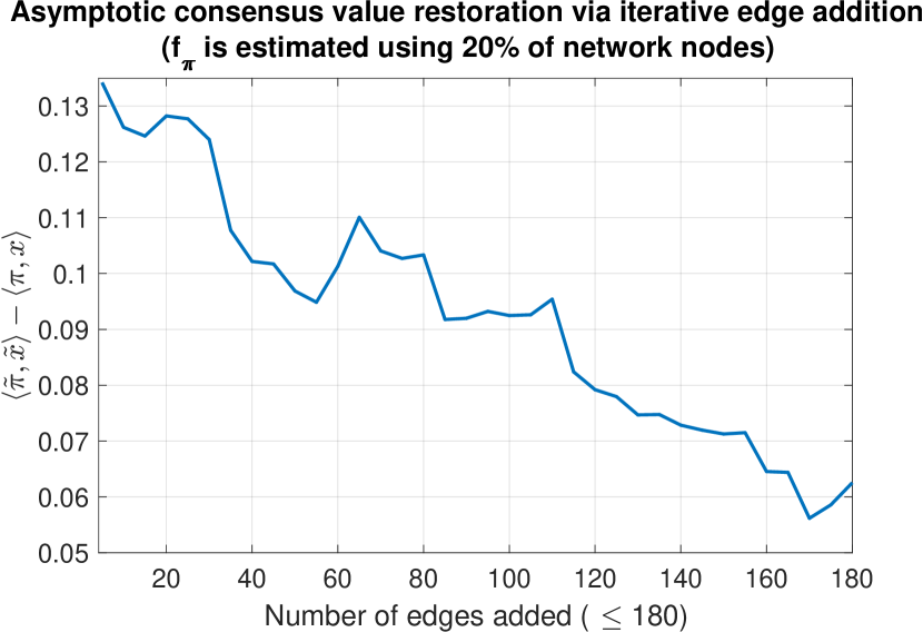
(c)

(d)

Figure 8: Solving $\operatorname{DIVER}$ via iterative edge addition using Algorithm 1.

Figures 8(a) and 8(b) show the quality $f_{\pi}$ of the edges that were suggested by Algorithm 1 for addition to the network, where the edge quality is either estimated or computed exactly, respectively. In Fig. 8(a), we can see that, if $f_{\pi}$ are estimated using only 20% of top-centrality nodes in the computation, then a few “bad” edges are selected by the heuristic, but most of the added edges are top-quality (have large values of $f_{\pi}$). In Fig. 8(b), for the case of exact computation of $f_{\pi}$, all added edges are top-quality, though, a small number of top-quality edges are missed, because their source nodes are not among the $n_{src}$ ones considered.

Fig. 8(c) and Fig. 8(d) show how $\operatorname{DIVER}$’s objective changes during iterative edge addition, when $f_{\pi}$ are either estimated or computed exactly. When we use exact $f_{\pi}$ (Fig. 8(d)), it takes 17 iterations (85 new edges) to drive the asymptotic consensus value $\langle\widetilde{\pi},\widetilde{x}\rangle$ back close to its original state $\langle\pi,x\rangle$. In case of using estimates of $f_{\pi}$ (Fig. 8(c)), the process stops having reached the allowed maximum of 180 new edges, and the asymptotic consensus value $\langle\widetilde{\pi},\widetilde{x}\rangle$ gets within $\approx 0.06$ (10%) of its original state $\langle\pi,x\rangle$.

7 Discussion and Future Work

In this work, we have formulated $\operatorname{DIVER}$—a problem of strategically adding edges to the network in order to disable the effect of external influence altering opinions of select users. Using a functional reduction from the classic subset sum problem, we have proven that this problem is NP-hard even for the case of undirected networks. Due to the problem’s hardness, we have focused on designing a heuristic for it. To that end, we have provided a perturbation analysis, formally answering the question of how the network nodes’ eigencentralities and, hence, $\operatorname{DIVER}$’s objective function change when a single edge is added to the network. The latter analysis led to the definition of candidate edge scores, that quantify the potential impact of the candidate edges, allowing to add them to the network in a greedy fashion. We have also provided insights into how to compute these edge scores in scale-free-like networks in pseudo-constant time, resulting in a pseudo-linear-time heuristic for $\operatorname{DIVER}$. One of these insights is related to efficiently estimating mean first passage times in Markov chains to and from high-centrality states. We have confirmed our theoretical findings in experiments.

Our results are rather general, and the provided insights and theory can be applied to other problems of strategically manipulating eigenvector centrality in networks. Simultaneously, this work opens many avenues for potential future research, including the following.

$\boldsymbol{\triangleright}$ $\operatorname{DIVER}$ targets optimization of the scalar asymptotic consensus value, being the value to which all the opinions asymptotically converge under DeGroot model. It is possible to generalize $\operatorname{DIVER}$ to the case of such opinion dynamics models as Friedkin-Johnsen [54] or the non-linear DeGroot model [55], where the users asymptotically disagree, and, hence, we need to optimize the asymptotic opinion distribution, rather than a scalar.

$\boldsymbol{\triangleright}$ For the purposes of efficiently computing potential impact of candidate edge addition, we have studied the question of how to efficiently estimate mean first passage times to or from top-centrality states in a Markov chain. While our answer to the latter question was based on an empirical study on scale-free networks, providing formal convergence bounds for MFPT estimation would benefit many scientific areas dealing with Markov processes.

$\boldsymbol{\triangleright}$ Finally, while $\operatorname{DIVER}$ was proposed as a method for fighting external influence upon the opinions of a social network’s users, it clearly can be used as an influence tool. Thus, it would be fruitful to study the ways to identify whether an edge recommendation process in a social network targets strategic change of the opinion distribution.

References

- [1] L. Festinger, “A theory of social comparison processes,” Human Relations, vol. 7, no. 2, pp. 117–140, 1954.
- [2] P. Domingos and M. Richardson, “Mining the network value of customers,” in Proc. of International Conference on Knowledge Discovery and Data Mining (KDD), pp. 57–66, ACM, 2001.
- [3] M. H. DeGroot, “Reaching a consensus,” Journal of the American Statistical Association, vol. 69, no. 345, pp. 118–121, 1974.
- [4] R. P. Abelson, “Mathematical models of the distribution of attitudes under controversy,” Contributions to Mathematical Psychology, vol. 14, pp. 1–160, 1964.
- [5] L. Festinger, A Theory of Cognitive Dissonance, vol. 2. Stanford University Press, 1962.
- [6] F. Heider, “Attitudes and cognitive organization,” The Journal of Psychology, vol. 21, no. 1, pp. 107–112, 1946.
- [7] D. Cartwright and F. Harary, “Structural balance: A generalization of Heider’s theory,” Psychological Review, vol. 63, no. 5, p. 277, 1956.
- [8] J. G. Kemeny and J. L. Snell, Finite Markov Chains. Springer, 1976.
- [9] V. Amelkin, P. Bogdanov, and A. K. Singh, “A distance measure for the analysis of polar opinion dynamics in social networks,” in Proc. International Conference on Data Engineering (ICDE), pp. 159–162, IEEE, 2017.
- [10] R. M. Karp, “Reducibility among combinatorial problems,” in Complexity of Computer Computations, pp. 85–103, Springer, 1972.
- [11] A. Ghosh and S. Boyd, “Growing well-connected graphs,” in Proc. of Conf. on Decision and Control, pp. 6605–6611, IEEE, 2006.
- [12] R. Merris, “Laplacian matrices of graphs: A survey,” Linear Algebra and Its Applications, vol. 197, pp. 143–176, 1994.
- [13] Z. Yu, C. Wang, J. Bu, X. Wang, Y. Wu, and C. Chen, “Friend recommendation with content spread enhancement in social networks,” Information Sciences, vol. 309, pp. 102–118, 2015.
- [14] P. Van Mieghem, D. Stevanović, F. Kuipers, C. Li, R. Van De Bovenkamp, D. Liu, and H. Wang, “Decreasing the spectral radius of a graph by link removals,” Physical Review E, vol. 84, no. 1, p. 016101, 2011.
- [15] S. Saha, A. Adiga, B. A. Prakash, and A. K. S. Vullikanti, “Approximation algorithms for reducing the spectral radius to control epidemic spread,” in Proc. of International Conference on Data Mining (SDM), pp. 568–576, SIAM, 2015.
- [16] Y. Zhang, A. Adiga, A. Vullikanti, and B. A. Prakash, “Controlling propagation at group scale on networks,” in Proc. of International Conference on Data Mining (ICDM), pp. 619–628, IEEE, 2015.
- [17] H. Tong, B. A. Prakash, T. Eliassi-Rad, M. Faloutsos, and C. Faloutsos, “Gelling, and melting, large graphs by edge manipulation,” in Proc. of International Conference on Information and Knowledge Management (CIKM), pp. 245–254, ACM, 2012.
- [18] C. Chen, H. Tong, B. A. Prakash, T. Eliassi-Rad, M. Faloutsos, and C. Faloutsos, “Eigen-optimization on large graphs by edge manipulation,” ACM Transactions on Knowledge Discovery from Data (TKDD), vol. 10, no. 4, p. 49, 2016.
- [19] L. T. Le, T. Eliassi-Rad, and H. Tong, “MET: A fast algorithm for minimizing propagation in large graphs with small eigen-gaps,” in Proc. of International Conference on Data Mining (SDM), pp. 694–702, SIAM, 2015.
- [20] H. Chan, L. Akoglu, and H. Tong, “Make it or break it: Manipulating robustness in large networks,” in Proc. of International Conference on Data Mining (SDM), pp. 325–333, SIAM, 2014.
- [21] A. Ghosh, S. Boyd, and A. Saberi, “Minimizing effective resistance of a graph,” SIAM Review, vol. 50, no. 1, pp. 37–66, 2008.
- [22] F. Arrigo and M. Benzi, “Updating and downdating techniques for optimizing network communicability,” SIAM Journal on Scientific Computing, vol. 38, no. 1, pp. 25–49, 2016.
- [23] K. Garimella, G. De Francisci Morales, A. Gionis, and M. Mathioudakis, “Reducing controversy by connecting opposing views,” in Proc. of International Conference on Web Search and Data Mining (WSDM), pp. 81–90, ACM, 2017.
- [24] V. Chaoji, S. Ranu, R. Rastogi, and R. Bhatt, “Recommendations to boost content spread in social networks,” in Proc. of International Conference on World Wide Web (WWW), pp. 529–538, ACM, 2012.
- [25] C. J. Kuhlman, G. Tuli, S. Swarup, M. V. Marathe, and S. Ravi, “Blocking simple and complex contagion by edge removal,” in Proc. of International Conference on Data Mining (ICDM), pp. 399–408, IEEE, 2013.
- [26] E. B. Khalil, B. Dilkina, and L. Song, “Scalable diffusion-aware optimization of network topology,” in Proc. of International Conference on Knowledge Discovery and Data Mining (KDD), pp. 1226–1235, ACM, 2014.
- [27] C. A. Phillips, “The network inhibition problem,” in Proc. of Symposium on Theory of Computing, pp. 776–785, ACM, 1993.
- [28] E. Israeli and R. K. Wood, “Shortest-path network interdiction,” Networks, vol. 40, no. 2, pp. 97–111, 2002.
- [29] M. Papagelis, F. Bonchi, and A. Gionis, “Suggesting ghost edges for a smaller world,” in Proc. of International Conference on Information and Knowledge Management (CIKM), pp. 2305–2308, ACM, 2011.
- [30] V. Ishakian, D. Erdös, E. Terzi, and A. Bestavros, “A framework for the evaluation and management of network centrality,” in Proc. of International Conference on Data Mining (SDM), pp. 427–438, SIAM, 2012.
- [31] N. Parotsidis, E. Pitoura, and P. Tsaparas, “Centrality-aware link recommendations,” in Proc. of International Conference on Web Search and Data Mining (WSDM), pp. 503–512, ACM, 2016.
- [32] S. Perumal, P. Basu, and Z. Guan, “Minimizing eccentricity in composite networks via constrained edge additions,” in Proc. of Military Communications Conference (MILCOM), pp. 1894–1899, IEEE, 2013.
- [33] S. Medya, A. Silva, A. Singh, P. Basu, and A. Swami, “Maximizing coverage centrality via network design,” in Proc. of International Conference on Knowledge Discovery and Data Mining (KDD), ACM, 2017.
- [34] K. Avrachenkov and N. Litvak, “The effect of new links on Google PageRank,” Stochastic Models, vol. 22, no. 2, pp. 319–331, 2006.
- [35] C. de Kerchove, L. Ninove, and P. Van Dooren, “Maximizing PageRank via outlinks,” Linear Algebra and its Applications, vol. 429, no. 5-6, pp. 1254–1276, 2008.
- [36] B. C. Csáji, R. M. Jungers, and V. D. Blondel, “PageRank optimization by edge selection,” Discrete Applied Mathematics, vol. 169, pp. 73–87, 2014.
- [37] H. Ishii and R. Tempo, “Computing the PageRank variation for fragile web data,” SICE Journal of Control, Measurement, and System Integration, vol. 2, no. 1, pp. 1–9, 2009.
- [38] M. Ye, J. Liu, B. Anderson, C. Yu, and T. Başar, “Modification of social dominance in social networks by selective adjustment of interpersonal weights,” arXiv:1703.03166, 2017.
- [39] P. Jia, A. MirTabatabaei, N. E. Friedkin, and F. Bullo, “Opinion dynamics and the evolution of social power in influence networks,” SIAM Review, vol. 57, no. 3, pp. 367–397, 2015.
- [40] G. E. Cho and C. D. Meyer, “Markov chain sensitivity measured by mean first passage times,” Linear Algebra and its Applications, vol. 316, no. 1-3, pp. 21–28, 2000.
- [41] S. Chien, C. Dwork, R. Kumar, and D. Sivakumar, “Towards exploiting link evolution,” in Workshop on Algorithms and Models for the Web Graph, 2001.
- [42] G. Jeh and J. Widom, “Scaling personalized web search,” in Proc. of International Conference on World Wide Web (WWW), pp. 271–279, ACM, 2003.
- [43] A. N. Langville and C. D. Meyer, “Updating Markov chains with an eye on Google’s PageRank,” SIAM Journal on Matrix Analysis and Applications, vol. 27, no. 4, pp. 968–987, 2006.
- [44] J. J. Hunter, “Stationary distributions and mean first passage times of perturbed Markov chains,” Linear Algebra and its Applications, vol. 410, no. 1-3, pp. 217–243, 2005.
- [45] G. Como and F. Fagnani, “Robustness of large-scale stochastic matrices to localized perturbations,” IEEE Transactions on Network Science and Engineering, vol. 2, no. 2, pp. 53–64, 2015.
- [46] B. Bahmani, R. Kumar, M. Mahdian, and E. Upfal, “PageRank on an evolving graph,” in Proc. of International Conference on Knowledge Discovery and Data Mining (KDD), pp. 24–32, ACM, 2012.
- [47] L. Li, H. Tong, Y. Xiao, and W. Fan, “Cheetah: Fast graph kernel tracking on dynamic graphs,” in Proc. of International Conference on Data Mining (SDM), pp. 280–288, SIAM, 2015.
- [48] C. Chen and H. Tong, “On the eigen-functions of dynamic graphs: Fast tracking and attribution algorithms,” Statistical Analysis and Data Mining: The ASA Data Science Journal, vol. 10, no. 2, pp. 121–135, 2017.
- [49] M.-J. Lee, J. Lee, J. Y. Park, R. H. Choi, and C.-W. Chung, “QUBE: A quick algorithm for updating betweenness centrality,” in Proc. of International Conference on World Wide Web (WWW), pp. 351–360, ACM, 2012.
- [50] A. E. Sariyüce, K. Kaya, E. Saule, and Ü. V. Çatalyürek, “Incremental algorithms for network management and analysis based on closeness centrality,” arXiv:1303.0422 [cs.DS], 2013.
- [51] J. J. Hunter, “The computation of the mean first passage times for Markov chains,” arXiv:1701.07781v2 [math.NA], 2017.
- [52] S. White and P. Smyth, “Algorithms for estimating relative importance in networks,” in Proc. of International Conference on Knowledge Discovery and Data Mining (KDD), pp. 266–275, ACM, 2003.
- [53] K. Avrachenkov, N. Litvak, D. Nemirovsky, and N. Osipova, “Monte Carlo methods in PageRank computation: When one iteration is sufficient,” SIAM Journal on Numerical Analysis, vol. 45, no. 2, pp. 890–904, 2007.
- [54] N. E. Friedkin and E. C. Johnsen, “Social influence networks and opinion change,” Advances in Group Processes, vol. 16, no. 1, pp. 1–29, 1999.
- [55] V. Amelkin, F. Bullo, and A. K. Singh, “Polar opinion dynamics in social networks,” IEEE Transactions on Automatic Control, vol. 62, Nov. 2017.