Higher-order sub-Poissonian-like nonclassical fields: Theoretical and experimental comparison

Abstract

Criteria defining higher-order sub-Poissonian-like fields are given using five different quantities: moments of I) integrated intensity, II) photon number, III) integrated-intensity fluctuation, IV) photon-number fluctuation, and V) elements of photocount and photon-number distributions. Relations among the moment criteria are revealed. Performance of the criteria is experimentally investigated using a set of potentially sub-Poissonian fields obtained by post-selection from a twin beam. The criteria based on moments of integrated intensity and photon number and those using the elements of photocount distribution are found as the most powerful. States nonclassical up to the fifth order are experimentally reached in the former case, even the ninth-order non-classicality is observed in the latter case.

Nonclassical properties of optical fields and their characterization have been in the center of attention from the beginning of quantum optics. The simplest, and from the experimental point of view the most natural, way how to achieve this is based on the determination of second-order moments of fluctuations of the measured quantities, that violate certain inequalities for nonclassical fields. This approach resulted in the introduction of principal squeeze variance of electric-field amplitudes and the Fano factor to quantify nonclassical phase fluctuations and photon-number fluctuations, respectively Luks1988 ; Davidovich1996 . The Fano factor represents the most important quantity for optical fields characterized by standard quadratic detectors, for which it identifies sub-Poissonian fields. It has been used to quantify nonclassical light originating in resonance fluorescence Kimble1977 ; Short1983 , Franck–Hertz experiment Teich1985 , high-efficiency light-emitting diodes Tapster1987 , second-harmonic generation Li1994 ; Bajer1999 , parametric deamplification Li1995 , second-subharmonic generation Koashi1993 , feed-forward action on the beam Mertz1990 ; Kim1992 or light generated in micro-cavities by passing atoms Raimond2001 . Highly sub-Poissonian fields have also been reached by post-selection from cw Rarity1987 ; Laurat2003 ; Zou2006 and pulsed twin beams (TWB) Bondani2007 ; PerinaJr2013b ; Lamperti2014 ; Iskhakov2016 ; Harder2016 .

The Fano factor $F$ defined in terms of photon-number moments as $F=\langle(\Delta\hat{n})^{2}\rangle/\langle\hat{n}\rangle$ identifies sub-Poissonian fields if $F<1$; $\Delta\hat{n}\equiv\hat{n}-\langle\hat{n}\rangle$ denotes the fluctuation of photon-number operator $\hat{n}$ given in terms of the annihilation ($\hat{a}$) and creation ($\hat{a}^{\dagger}$) operators as $\hat{n}\equiv\hat{a}^{\dagger}\hat{a}$. Symbol $\langle\rangle$ stands for the mean value. This condition when expressed in the moments of integrated intensity $W$ (or equivalently in the normally-ordered moments of photon number, i.e. $\langle W^{k}\rangle\equiv\langle\hat{a}^{\dagger k}\hat{a}^{k}\rangle$ Perina1991 ; Saleh1978 ; Vogel2006 ), $\langle(\Delta W)^{2}\rangle=\langle\hat{a}^{\dagger 2}\hat{a}^{2}\rangle-\langle\hat{a}^{\dagger}\hat{a}\rangle^{2}<0$ [for the relation between the moments that is used for determining intensity moments from the experimental data, see Eq. (3) below], reveals the relation with the general definition of non-classicality: A field is nonclassical provided that its (normally-ordered) Glauber-Sudarshan quasi-distribution ${\cal P}$ (as a function of complex field amplitudes) attains negative values or even does not exist as a regular function Glauber1963 ; Sudarshan1963 . The consideration of the marginal quasi-distribution $P$ of integrated intensities, application of this definition to any classical field and use of the Cauchy-Schwarz inequality (or the majorization theory Lee1990a ) result in the chain of inequalities $\langle W^{k}\rangle>\langle W\rangle^{k}$ fulfilled by any classical field. These inequalities then allow to naturally define a $k$-th order non-classicality (with respect to intensity $W$) Mista1977 ; Perina1991 ; Hong1985b ; Prakash2006 ; Verma2010 according to the following Criteria I:

$$r_{W}^{(k)}\equiv\langle W^{k}\rangle/\langle W\rangle^{k}-1<0,\hskip 14.22636ptk=2,\ldots.$$ (1)

As the quasi-distribution $P$ of integrated intensity completely describes the field intensity, we consider the definition (1) of higher-order non-classicalities as the most fundamental. We note that different kinds of higher-order non-classicalities have been defined when considering powers of complex field amplitudes Hong1985a ; Hillery1987a ; Hillery1987b .

On the other hand, photon-number-resolving detectors straightforwardly provide the moments of photon number $\hat{n}$. The following sequence of non-classicality Criteria II can be defined using these moments:

$$r_{n}^{(k)}\equiv\langle\hat{n}^{k}\rangle/\langle\hat{n}^{k}\rangle_{\rm Pois}-1<0,\hskip 14.22636ptk=2,\ldots.$$ (2)

The moments $\langle\hat{n}^{k}\rangle_{\rm Pois}$ characterize a Poissonian field (in a coherent state) with mean photon number $\langle\hat{n}\rangle$. Indeed, the relation among both types of moments expressed via the Stirling numbers $S_{k}^{l}$ of the second kind ($k\geq 1$),

$$\langle\hat{n}^{k}\rangle=\sum_{l=1}^{k}S_{k}^{l}\langle W^{l}\rangle,\hskip 8.53581ptS_{k}^{l}\equiv\frac{1}{l!}\sum_{m=0}^{l}(-1)^{l-m}\left(\begin{array}[]{c}l\\ m\end{array}\right)m^{k},$$ (3)

allows to rewrite criteria (2) into the form:

$$\langle\hat{n}^{k}\rangle-\langle\hat{n}^{k}\rangle_{\rm Pois}=\sum_{l=1}^{k}S_{k}^{l}\left(\langle W^{k}\rangle-\langle W\rangle^{k}\right)<0.$$ (4)

The relation (4) together with positivity of the Stirling numbers $S$ confirm that criteria (2) express non-classicality. Whereas Criteria I in Eqs. (1) and II in Eqs. (2) are identical for $k=2$, they represent in general different definitions of a $k$-th order non-classicality. For example, a field obeying $\langle W^{3}\rangle-\langle W\rangle^{3}<0$ does not have to fulfill the condition $\langle\hat{n}^{3}\rangle-\langle\hat{n}^{3}\rangle_{\rm Poiss}<0$ and vice versa. Both Criteria I and II approach each other only for intense fields ($\langle W\rangle\gg 1$) for which the last term in the sum in Eq. (4) dominates ($S_{k}^{k}=1$ for $k=1,\ldots$).

Non-classicality of an optical field can also be revealed by the moments of intensity ($\Delta W\equiv W-\langle W\rangle$) and photon-number ($\Delta\hat{n}\equiv\hat{n}-\langle\hat{n}\rangle$) fluctuations. This leads us to the following Criteria III and IV:

$$r_{\Delta W}^{(k)} \equiv \langle(\Delta W)^{k}\rangle/\langle W\rangle^{k},$$ (5)

$$r_{\Delta n}^{(k)} \equiv \langle(\Delta\hat{n})^{k}\rangle/\langle(\Delta\hat{n})^{k}\rangle_{\rm Pois}-1,\hskip 14.22636ptk=2,\ldots.$$ (6)

We note that $\langle(\Delta\hat{n})^{2}\rangle_{\rm Pois}=\langle(\Delta\hat{n})^{3}\rangle_{\rm Pois}=\langle\hat{n}\rangle$, $\langle(\Delta\hat{n})^{4}\rangle_{\rm Pois}=\langle\hat{n}\rangle+3\langle\hat{n}\rangle^{2}$ and $\langle(\Delta\hat{n})^{5}\rangle_{\rm Pois}=\langle\hat{n}\rangle+10\langle\hat{n}\rangle^{2}$. However, Criteria III $r_{\Delta W}^{(k)}<0$ for intensity fluctuations are applicable only for even orders $k$. Also Criteria IV $r_{\Delta n}^{(k)}<0$ reveal non-classicality only for fields with mean intensities $\langle W\rangle$ lower than certain value. A detailed analysis of expressions $\langle(\Delta\hat{n})^{k}\rangle-\langle(\Delta\hat{n})^{k}\rangle_{\rm Pois}$ rewritten as polynomials of $k$-th order in $\Delta W$ with $\langle W\rangle$ considered as a parameter Kim1998 gives $r_{\Delta n}^{(3)}<0$ as a non-classicality indicator for $\langle W\rangle<3$ and $r_{\Delta n}^{(4)}<0$ for arbitrary intensities.

Formally similar non-classicality criteria are derived for the elements $p(k)$ of photon-number distribution Klyshko1996 . These elements, given by the Mandel detection formula Perina1991 ; Saleh1978

$$p(k)=\int_{0}^{\infty}dW\,W^{k}\exp(-W)P(W)/k!,$$ (7)

represent ’un-normalized’ moments that obey, according to the majorization theory, certain inequalities for non-negative distribution $P(W)$ of integrated intensity Klyshko1996 ; Lee1998 . Nonclassical fields are then identified by their violation, which allows us to formulate Criteria V in terms of the modified elements $\tilde{p}(k)\equiv k!p(k)/p(0)$, $k=1,2,\ldots$, as follows:

$$r_{p}^{(k)}\equiv\tilde{p}(k)/\tilde{p}(1)^{k}-1<0,\hskip 14.22636ptk=2,\ldots.$$ (8)

For a Poissonian field, we have $r_{p}^{(k)}=0$ for all $k$. Moreover, the majorization theory allows to derive a larger number of non-classicality inequalities among the elements $\tilde{p}(k)$, in tight parallel with those for intensity moments $\langle W^{k}\rangle$ analyzed for $k\leq 5$ in Arkhipov2016c .

Criterion I $r_{W}^{(k)}<0$ for a $k$-th order non-classicality can be converted into the $k$-th-order non-classicality depth $\tau^{(k)}$ Lee1991 using the formula

$$\tau^{(k)}=(1-s^{(k)}_{\rm th})/2,$$ (9)

where $s^{(k)}_{\rm th}$ gives the threshold value of the ordering parameter $s$ for which $\langle W^{k}\rangle_{s}=\langle W\rangle^{k}_{s}$. The $s$-ordered moments $\langle W^{k}\rangle_{s}$ of intensity $W$, which are determined along the usual way considering an $s$-ordered quasi-distribution $\tilde{P}(W;s)$ of integrated intensity [see below], are expressed in terms of the usual normally-ordered moments ($s=1$) as follows Perina1991 ; Vogel2006 :

$$\langle W^{k}\rangle_{s}=\left(\frac{2}{1-s}\right)^{k}\left\langle{\rm L}_{k}\left(\frac{2W}{s-1}\right)\right\rangle;$$ (10)

${\rm L}_{k}$ denotes a $k$-th Laguerre polynomial Gradshtein2000 . We note that such moments are appropriate for a field into which a thermal field with $(1-s)$ mean photon number is added. Contrary to the parameters $r_{W}^{(k)}$ the non-classicality depths $\tau^{(k)}$ of different orders can be mutually directly compared. The greater the value of $\tau^{(k)}$ is the stronger the non-classicality is.

The parameters $r_{W}^{(k)}$ naturally occur when determining the declination $\Delta\tilde{P}(W;s)$ of an $s$-ordered quasi-distribution $\tilde{P}(W;s)$ of integrated intensity from that belonging to the Poissonian field, which is denoted as $\tilde{P}_{\rm Pois}(W;s)$ Perina1991 :

$$\Delta\tilde{P}(W;s) = \exp\left(-\frac{W}{\langle W\rangle}\right)\sum_{j=0}^{\infty}c_{j}{\rm L}_{j}\left(-\frac{W}{\langle W\rangle}\right),$$

$$c_{j} = \frac{j!}{\langle W\rangle}\sum_{l=0}^{j}\frac{(-1)^{l}r_{W}^{(l)}}{(l!)^{2}(j-l)!}.$$ (11)

It holds that $\int_{0}^{\infty}dW\Delta\tilde{P}(W;s)=0$ and so $\Delta\tilde{P}(W;s)$ of any non-Poissonian field has to have negative values. However, negative values of a non-classical field occur in the regions where they cannot be compensated by positive values of the Poissonian distribution $\tilde{P}_{\rm Pois}(W;s)$.

The performance of different non-classicality quantifiers has been experimentally tested on a set of 10 potentially sub-Poissonian fields obtained by post-selection from a TWB. The used TWB was generated in a nonlinear crystal and its signal and idler fields were detected in different regions of an iCCD camera PerinaJr2012 (for details, see Fig. 1). The signal photocounts were used for the post-selection process: Detection of a given number $c_{\rm s}$ of signal photocounts ideally leaves the idler field in the state with $c_{\rm i}=c_{\rm s}$ idler photons. Under real experimental conditions, the post-selected idler field exhibits fluctuations in photon numbers that, however, are under suitable conditions smaller than those characterizing the corresponding Poissonian field. The post-selected idler fields were measured via their photocount distributions monitored by the iCCD camera. The obtained post-selected idler fields had different intensities as the mean number $\langle n_{\rm i}\rangle$ of idler photons increases with the increasing signal photocount number $c_{\rm s}$.

Moreover, as the experiment provided the whole 2D joint signal-idler photocount histogram $f(c_{\rm s},c_{\rm i})$ it also allowed to reconstruct the whole TWB. The TWB was reconstructed as a field composed of three independent components, one characterizing ideal photon pairs, one describing noisy signal photons and one belonging to noisy idler photons. Each component is characterized by mean photon(-pair) number $B_{a}$ per mode and number $M_{a}$ of independent modes, $a={\rm p,s,i}$, and its photon-number distribution is given by the Mandel-Rice formula Perina1991 ; Saleh1978 ; PerinaJr2013a . The distribution $p_{\rm si}(n_{\rm s},n_{\rm i})$ of the whole TWB is then expressed in the form of the following two-fold convolution PerinaJr2012a ; PerinaJr2013a ; Perina2005 :

$$p_{\rm si}(n_{\rm s},n_{\rm i}) = \sum_{n=0}^{{\rm min}[n_{\rm s},n_{\rm i}]}p(n_{\rm s}-n;M_{\rm s},B_{\rm s})p(n_{\rm i}-n;M_{\rm i},B_{\rm i})$$ (12)

$$\mbox{}\times p(n;M_{\rm p},B_{\rm p});$$

$p(n;M,B)=\Gamma(n+M)/[n!\,\Gamma(M)]B^{n}/(1+B)^{n+M}$ and symbol $\Gamma$ denotes the $\Gamma$-function.

For the reconstructed TWB, the theoretical post-selected idler photon-number distributions $p_{\rm c,i}^{\rm theo}(n_{\rm i};c_{\rm s})$ observed after detecting $c_{\rm s}$ signal photocounts are expected in the form (for details, see PerinaJr2013b ):

$$p_{\rm c,i}^{\rm theo}(n_{\rm i};c_{\rm s})=\frac{\sum_{n_{\rm s}}T_{\rm s}(c_{\rm s},n_{\rm s})p_{\rm si}(n_{\rm s},n_{\rm i})}{f_{\rm s}^{\rm theo}(c_{\rm s})}$$ (13)

where $f_{\rm s}^{\rm theo}(c_{\rm s})\equiv\sum_{n_{\rm s},n_{\rm i}}T_{\rm s}(c_{\rm s},n_{\rm s})p_{\rm si}(n_{\rm s},n_{\rm i})$ is the expected signal-field photocount distribution. Function $T_{\rm s}(c_{\rm s},n_{\rm s})$ occurring in Eq. (13) characterizes detection by the camera: It determines the probabilities of having $c_{\rm s}$ photocounts when detecting a field with $n_{\rm s}$ photons. For the used iCCD camera and both detection areas with $N_{a}$ active pixels, detection efficiencies $\eta_{a}$ and mean dark counts per pixel $D_{a}$, $a={\rm s,i}$, we have PerinaJr2012 :

$$T_{a}(c_{a},n_{a}) = \left(\begin{array}[]{c}N_{a}\\ c_{a}\end{array}\right)(1-D_{a})^{N_{a}}(1-\eta_{a})^{n_{a}}(-1)^{c_{a}}$$ (19)

$$\mbox{}\times\sum_{l=0}^{c_{a}}\left(\begin{array}[]{c}c_{a}\\ l\end{array}\right)\frac{(-1)^{l}}{(1-D_{a})^{l}}\left(1+\frac{l}{N_{a}}\frac{\eta_{a}}{1-\eta_{a}}\right)^{n_{a}}.$$

In the experiment, the photon-number distributions of the post-selected idler fields were reached by applying the maximum-likelihood approach (MLA) Dempster1977 . The photon-number distribution $p_{\rm c,i}(n_{\rm i};c_{\rm s})$ conditioned by detection of $c_{\rm s}$ signal photocounts has been found as a steady state of the following iteration procedure PerinaJr2012

$$p_{\rm c,i}^{(l+1)}(n_{\rm i};c_{\rm s}) = p_{\rm c,i}^{(l)}(n_{\rm i};c_{\rm s})\sum_{c_{\rm i}}\frac{f_{\rm i}(c_{\rm i};c_{\rm s})T_{\rm i}(c_{\rm i},n_{\rm i})}{\sum_{n^{\prime}_{i}}T_{\rm i}(c_{\rm i},n^{\prime}_{\rm i})p_{\rm c,i}^{(l)}(n^{\prime}_{\rm i};c_{\rm s})},$$ (20)

$$\hskip 42.67912ptl=0,1,\ldots.$$

In Eq. (20), the normalized idler-field 1D photocount histograms $f_{\rm i}(c_{\rm i};c_{\rm s})\equiv f(c_{\rm s},c_{\rm i})/f_{\rm s}(c_{\rm s})$ with the signal photocount histogram $f_{\rm s}(c_{\rm s})\equiv\sum_{c_{\rm i}}f(c_{\rm s},c_{\rm i})$ include the experimental realizations with $c_{\rm s}$ observed signal photocounts.

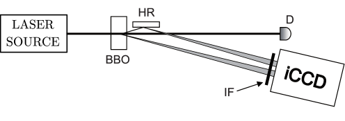
Figure 1: Scheme of the experimental setup: A TWB was emitted in non-collinear geometry in a 5-mm-long type-I BaB₂O₄ crystal (BBO) pumped by the third harmonics (280 nm) of a femtosecond cavity dumped Ti:sapphire laser (pulse duration 150 fs, central wavelength 840 nm, rep. rate 50 kHz, power 5 mW, collimated 1.5-mm-wide beam). The signal and idler (after reflection on a highly-reflecting mirror HR) fields generated by a single pump pulse were detected with detection efficiencies $\eta_{\rm s}=0.230\pm 0.005$ and $\eta_{\rm i}=0.220\pm 0.005$ by $N_{\rm s}=6528$ and $N_{\rm i}=6784$ pixels of the photocathode of iCCD camera Andor DH334-18U-63 with mean dark counts per pulse $d=0.04$ ($D_{a}=d/N_{a}$, $a={\rm s,i}$), rep. rate 10 Hz and integration time 4 ns. The nearly-frequency-degenerate signal and idler photons at the wavelength of 560 nm were filtered by a 14-nm-wide bandpass interference filter IF that defined the measured TWB with parameters $M_{\rm p}=270$, $B_{\rm p}=0.032$, $M_{\rm s}=0.01$, $B_{\rm s}=7.6$, $M_{\rm i}=0.026$, and $B_{\rm i}=5.3$ determined with relative error 7 % (for details, see PerinaJr2013a ); $\langle c_{\rm s}\rangle=2.20\pm 0.01$ and $\langle c_{\rm i}\rangle=2.18\pm 0.01$. Pump-beam intensity was actively stabilized via a motorized half-wave plate followed by a polarizer and monitored by detector D during $1.2\times 10^{6}$ repetitions of the measurement.

The experimental post-selection procedure provided ten different idler fields with different probabilities $f_{\rm s}(c_{\rm s})$ of realization [see Fig. 2(a)] and mean idler photon numbers $\langle n_{\rm c,i}\rangle$ increasing from 7 to 15 as the signal photocount number $c_{\rm s}$ used in the post-selection increases [see Fig. 2(b)]. In Fig. 2, and also in subsequent figures, we plot the quantities related to experimental photocounts (photon numbers reached by MLA) by red asterisks (green triangles) and those originating in the Gaussian fit of the TWB (GTWB) by blue solid curves. For comparison, we also depict by brown diamonds quantities reached by the simplest reconstruction method based on the intensity moments and relations $\langle W^{k}\rangle\rightarrow\langle W^{k}\rangle/\eta^{k}$. As this method does not take into account dark counts, it overestimates in general photon-number moments of the reconstructed distributions, as illustrated for the mean idler photon numbers $\langle n_{\rm i}\rangle$ in Fig. 2(b). As the experimental errors are linearly proportional to $1/\sqrt{N_{\rm rep}}$ with $N_{\rm rep}$ giving the number of measurement repetitions and according to the graph in Fig. 2(a), the characterization of the post-selected idler photon-number distributions with the signal photocount numbers $c_{\rm s}$ greater than 7 suffers from larger errors due to the low numbers of appropriate measurements, despite the large number of $1.2\times 10^{6}$ overall measurements made. We note that fixed detection efficiencies $\eta_{\rm s}$ and $\eta_{\rm i}$ were considered when determining the experimental errors of the analyzed criteria as their possible variations have only negligible influence to identification of non-classicality in the reconstructed states.

 

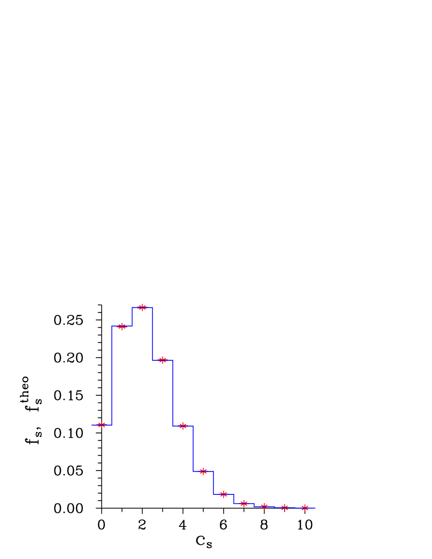
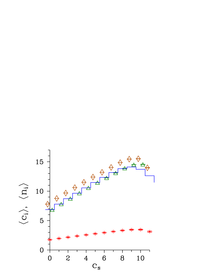
(a)                               (b)

Figure 2: (a) Signal photocount histogram $f_{\rm s}$ and its theoretical prediction $f_{\rm s}^{\rm theo}$ and (b) mean photocount (photon) number $\langle c_{\rm i}\rangle$ ($\langle n_{\rm i}\rangle$) of the post-selected idler fields as they depend on signal photocount number $c_{\rm s}$. Data for experimental photocount distributions (red $\ast$) and photon-number distributions determined by MLA (green $\triangle$), GTWB (blue solid curve) and modifying the intensity moments (brown $\diamond$) are plotted. Experimental errors are smaller than the used symbols.

Criteria I and II: Parameters $r_{W}^{(k)}$ quantifying $k$-th-order non-classicalities via the ’theoretical’ intensity moments and plotted in Figs. 3(a,c,e,g) show that the post-selected idler fields conditioned by the detected signal photocount numbers $c_{\rm s}$ in the range $\langle 3,7\rangle$ are nonclassical in the second and the third orders. Moreover the post-selected idler fields in the range $\langle 5,7\rangle$ are nonclassical in the fourth and the fifth orders. The comparison of intensity parameters $r_{W}^{(k)}$ with the corresponding ’experimental’ photon-number parameters $r_{n}^{(k)}$ based on the graphs in Fig. 3 reveals accordance in the occurrence of non-classicality of different orders indicated by both kinds of parameters for the measured photocount as well as the reconstructed photon-number quantities. The graphs in Fig. 3 also show that greater negative values of parameters $r_{W}^{(k)}$ and $r_{n}^{(k)}$ are systematically reached for the reconstructed photon-number distributions (by MLA and GTWB) in comparison with those arising in the photocount distributions. This is due to partial elimination of the noise by the reconstruction.

  

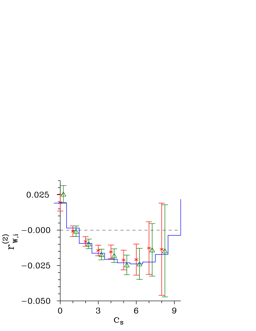
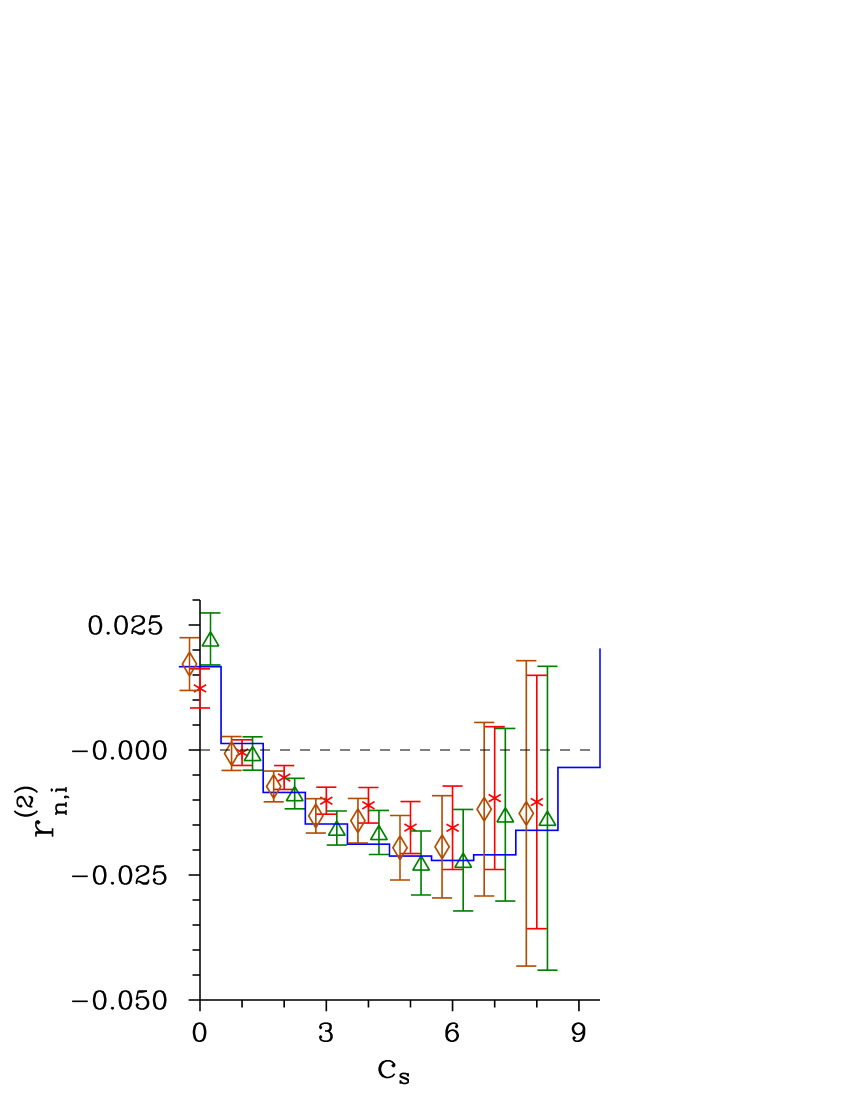
(a)                               (b)

  

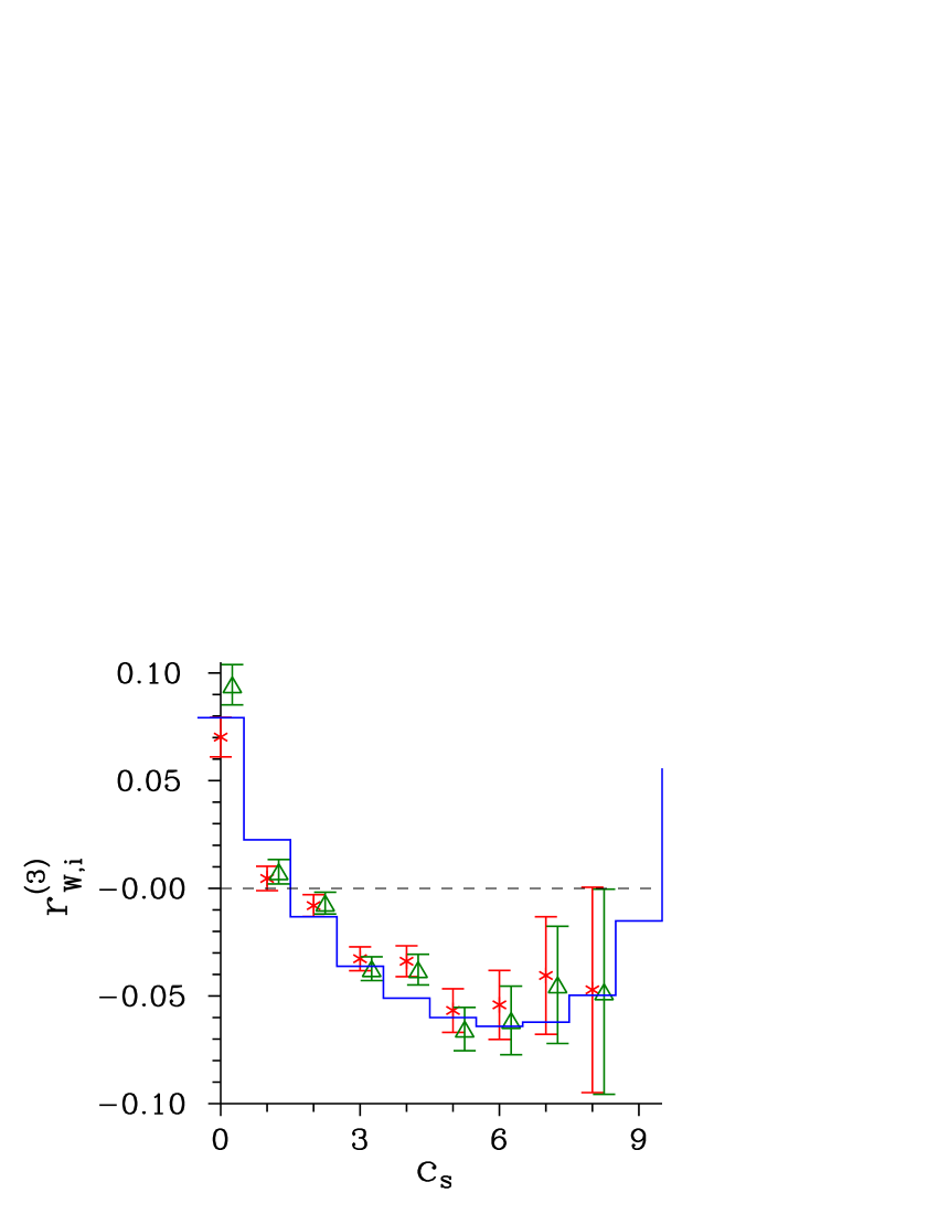
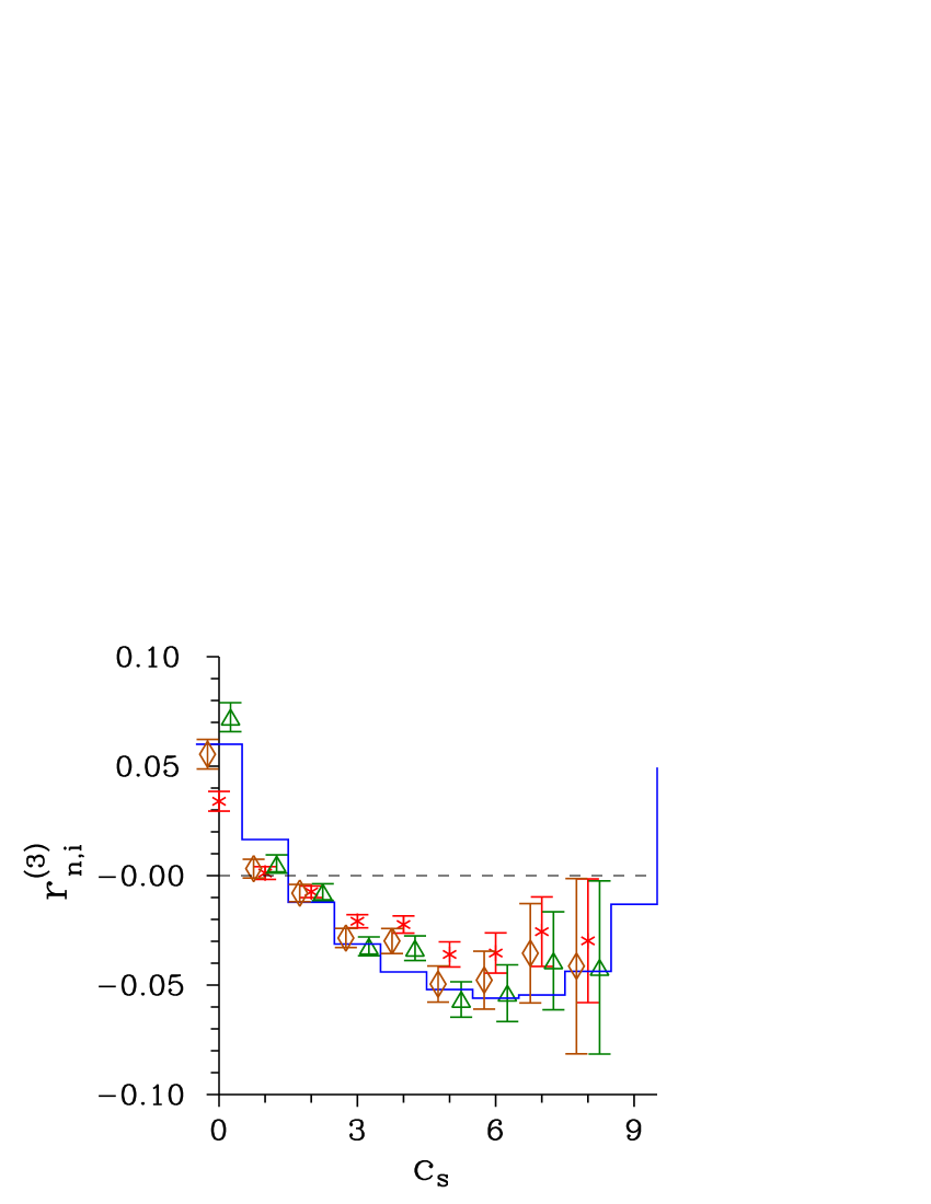
(c)                               (d)

  

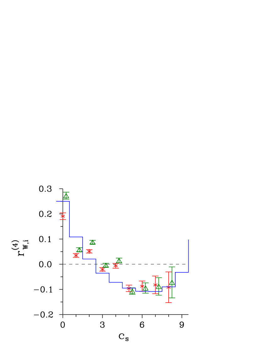
(e)                               (f)

  

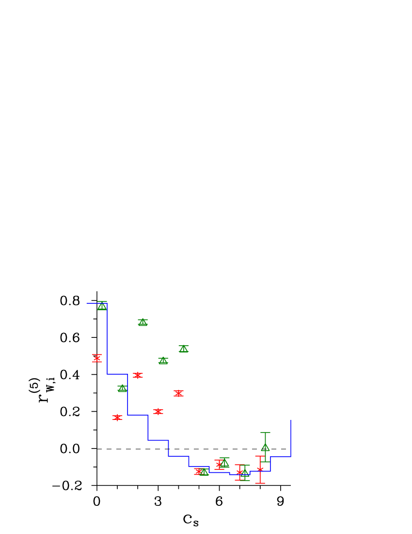
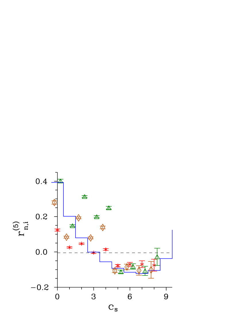
(g)                               (h)

Figure 3: Parameters $r_{W,{\rm i}}^{(k)}$ and $r_{n,{\rm i}}^{(k)}$ of the post-selected idler fields for $k=2$ (a,b), 3 (c,d), 4 (e,f), and 5 (g,h) as they depend on signal photocount number $c_{\rm s}$. The used symbols and curves are described in the caption to Fig. 2.

The non-classicalities of different orders are mutually compared in Fig. 4 via their non-classicality depths $\tau^{(k)}$ defined in Eq. (9). For the generated states, the greater the non-classicality order $k$ is the smaller the values $\tau^{(k)}$ of the corresponding non-classicality depths are observed and so the weaker the resistance of the non-classicality against the external noise is. As the directly measured photocount distributions give roughly 4-times lower intensities than the reconstructed photon-number distributions, the obtained values of non-classicality depths $\tau^{(k)}$ are naturally smaller for photocounts compared to photon numbers.

  

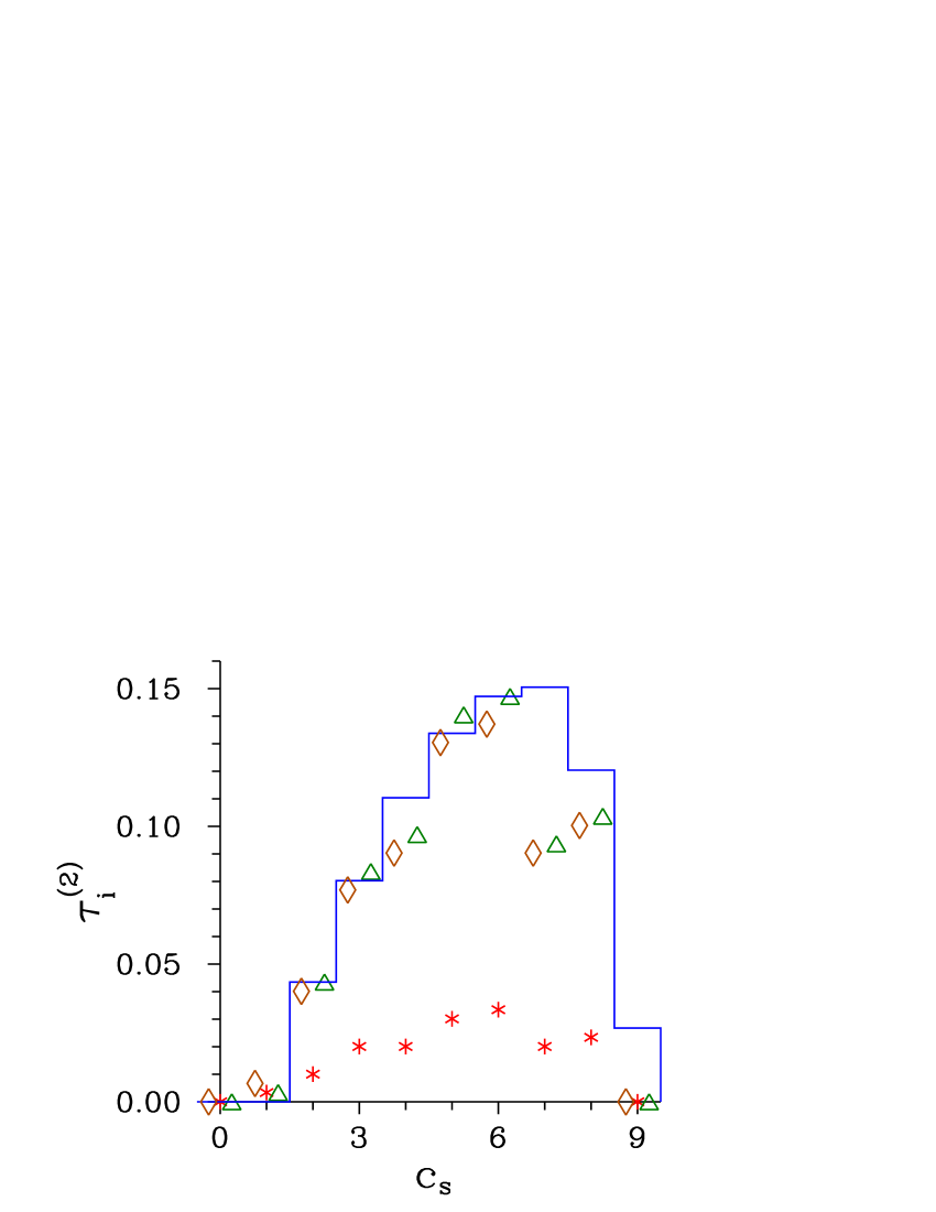
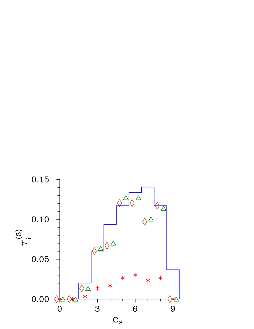
(a)                               (b)

  

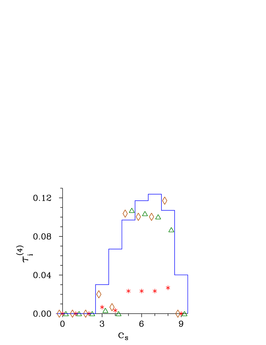
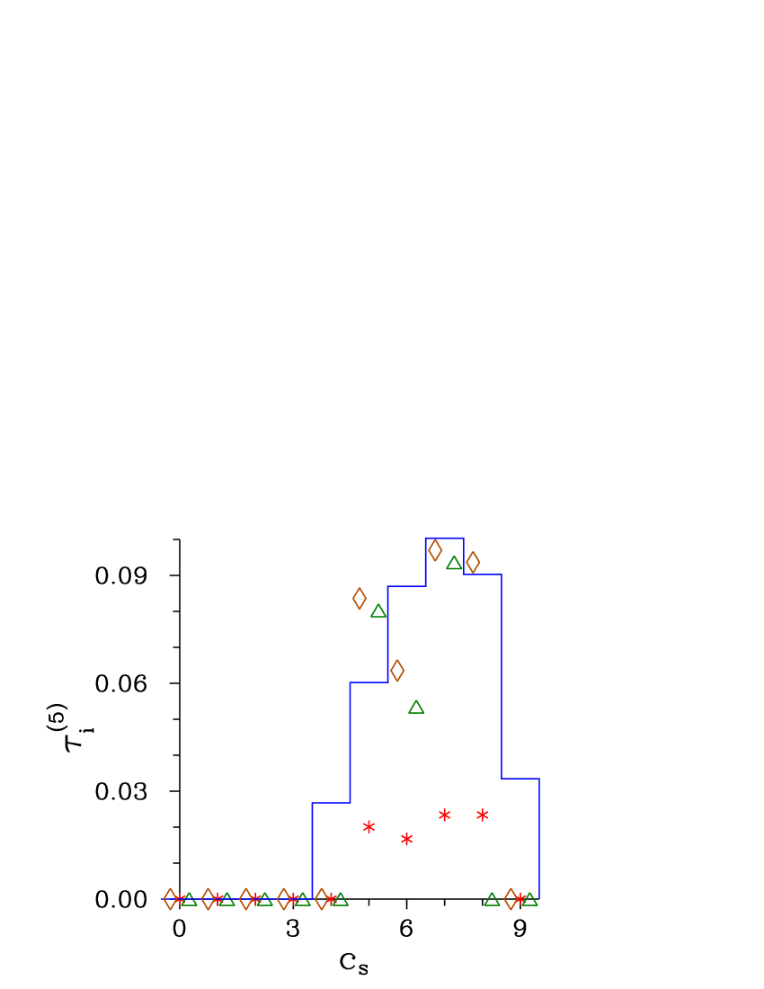
(c)                               (d)

Figure 4: Non-classicality depths $\tau_{\rm i}^{(k)}$ of the post-selected idler fields for $k=2$ (a), 3 (b), 4 (c), and 5 (d) as they depend on signal photocount number $c_{\rm s}$. The used symbols and curves are described in the caption to Fig. 2.

Criteria III and IV: Excluding the second-order non-classicalities for which the parameters $r_{\Delta W}^{(2)}$ and $r_{\Delta n}^{(2)}$ accord with the above analyzed parameters $r_{W}^{(2)}$ and $r_{n}^{(2)}$, the ability of both experimental and reconstructed moments of intensity and photocount (photon-number) fluctuations to reveal higher-order non-classicalities is qualitatively worse than that of parameters $r_{W}^{(k)}$ and $r_{n}^{(k)}$. This is due to large experimental errors and the reasons discussed below Eq. (6). As shown in Fig. 5, none of the non-classicality identifiers $r_{\Delta W}^{(4)}$, $r_{\Delta c}^{(3)}$ and $r_{\Delta c}^{(4)}$ reveals the post-selected idler fields as non-classical using the experimental photocounts and their errors.

  

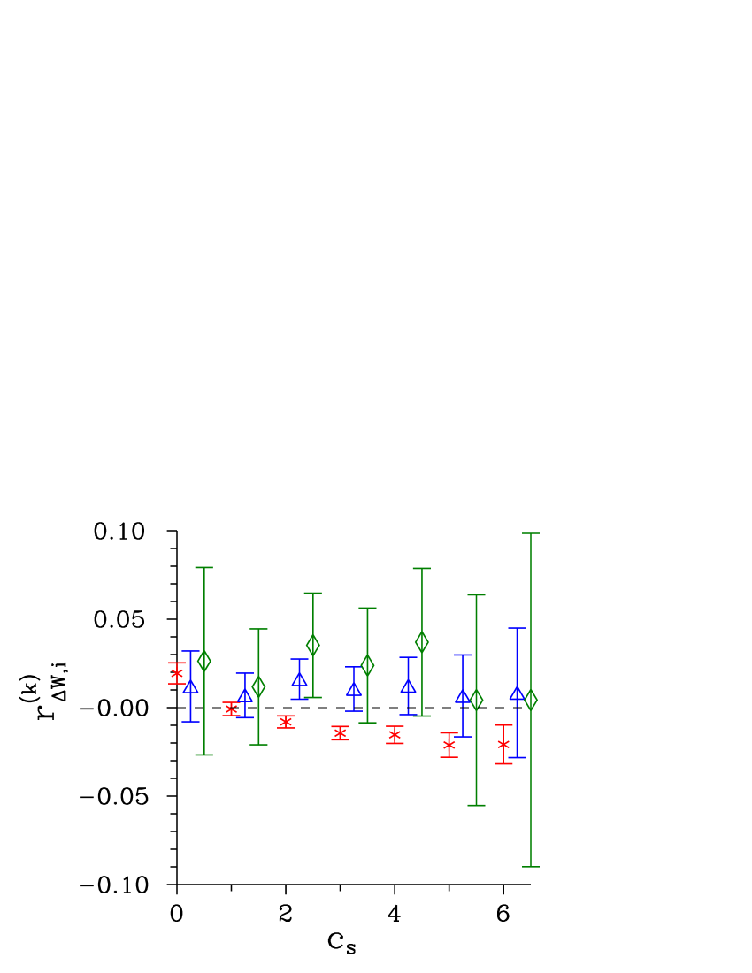
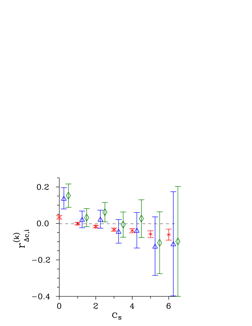
(a)                               (b)

Figure 5: Parameters $r_{\Delta W,{\rm i}}^{(k)}$ (a) and $r_{\Delta c,{\rm i}}^{(k)}$ (b) of the post-selected photocount idler fields for $k=2$ (red $\ast$), 3 (blue $\triangle$) and 4 (green $\diamond$) as they depend on signal photocount number $c_{\rm s}$.

Criterion V: From the point of view of experimental errors, the best results are found for the parameters $r_{p}^{(k)}$ defined in Eq. (8) and involving the elements $f_{\rm i}(c_{\rm i};c_{\rm s})$ of conditional idler photocount histograms, that represent a certain discrete transform of the moments $\langle c_{\rm i}^{l}\rangle$ for $l=0,1,\ldots,\infty$. The graphs presented in Fig. 6 document that we can recognize, within the experimental errors, the non-classicality up to the ninth order for idler fields post-selected by the signal photocount numbers $c_{\rm s}$ in the range $\langle 2,7\rangle$. Also, the idler field post-selected by the detection of $c_{\rm s}=1$ signal photocount is newly identified as nonclassical, even up to the fifth order. On the other hand, the reconstruction procedures performed for detection efficiency $\eta_{\rm i}\approx 0.2$ considerably amplify the fields and thus introduce larger errors. This disqualifies the application of parameters $r_{p}^{(k)}$ to the reconstructed fields.

  

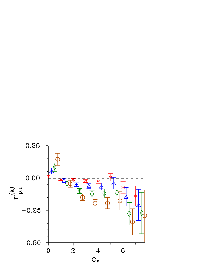
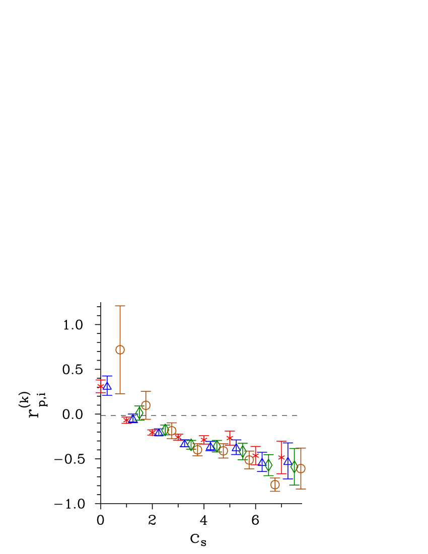
(a)                               (b)

Figure 6: Parameters $r_{p,{\rm i}}^{(k)}$ of the post-selected idler photocount histograms for (a) $k=2$ (red $\ast$), 3 (blue $\triangle$), 4 (green $\diamond$), and 5 (brown $\circ$) and (b) $k=6$ (red $\ast$), 7 (blue $\triangle$), 8 (green $\diamond$), and 9 (brown $\circ$) as they depend on signal photocount number $c_{\rm s}$.

At last, we present, as a typical example, the distributions characterizing the idler fields post-selected by the detection of $c_{\rm s}=5$ signal photocounts. The experimental idler photocount histogram $f_{\rm i}(c_{\rm i})$ is compared with the corresponding Poissonian distribution in Fig. 7(a). Similarly, the post-selected idler photon-number distributions $p_{\rm c,i}(n_{\rm i})$ reached by MLA and GTWB are compared with the appropriate Poissonian distribution in Fig. 7(b). Whereas the photocount histogram is very close to its Poissonian counterpart, the difference between the reconstructed photon-number distributions and the Poissonian distribution is well recognized.

  

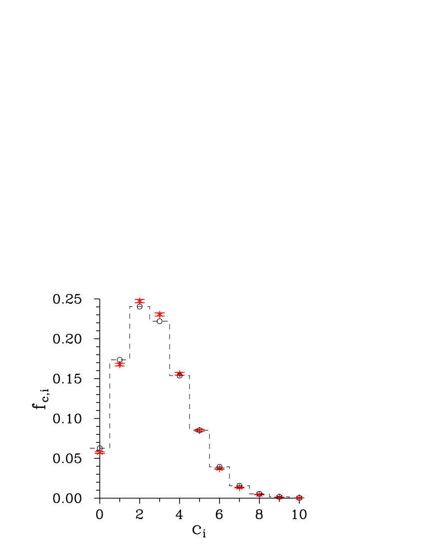
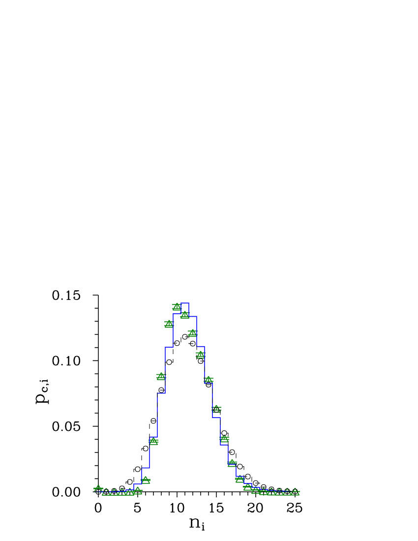
(a)                               (b)

Figure 7: (a) Idler photocount histogram $f_{\rm c,i}(c_{\rm i})\equiv f_{\rm i}(c_{\rm i};c_{\rm s})$ and (b) idler photon-number distributions $p_{\rm c,i}(n_{\rm i})$ post-selected by detection of $c_{\rm s}=5$ signal photocounts. The used symbols and blue curve are described in the caption to Fig. 2. For comparison, the corresponding Poissonian distributions are drawn by dashed curves with $\circ$.

The signs of intensity parameters $r_{W,s}^{(k)}$ defined in terms of $s$-ordered intensity moments qualitatively influence the shape of quasi-distribution $\tilde{P}_{\rm c,i}(W_{\rm i};s)$ of integrated intensity. If the parameters $r_{W,s}^{(k)}$ are negative, the difference $\Delta\tilde{P}_{\rm c,i}$ defined in Eq. (11) attains negative values in the regions where they are not compensated by positive values of the Poissonian distribution $\tilde{P}_{\rm Pois}$ and so the resultant quasi-distribution $\tilde{P}_{\rm c,i}(W_{\rm i};s)$ is nonclassical due to its negative values. This occurs for the ordering parameter $s$ greater than $s_{\rm th}^{(2)}$, as demonstrated in Fig. 8(a) for $s=0.9$. On the other hand, positive parameters $r_{W,s}^{(k)}$ observed for $s<s_{\rm th}^{(2)}$ cause ’redistribution’ of the classical probability densities of $\tilde{P}_{\rm c,i}(W_{\rm i};s)$ such that greater values occur for small intensities $W$ and the central peak lowers [see Fig. 8(b)].

  

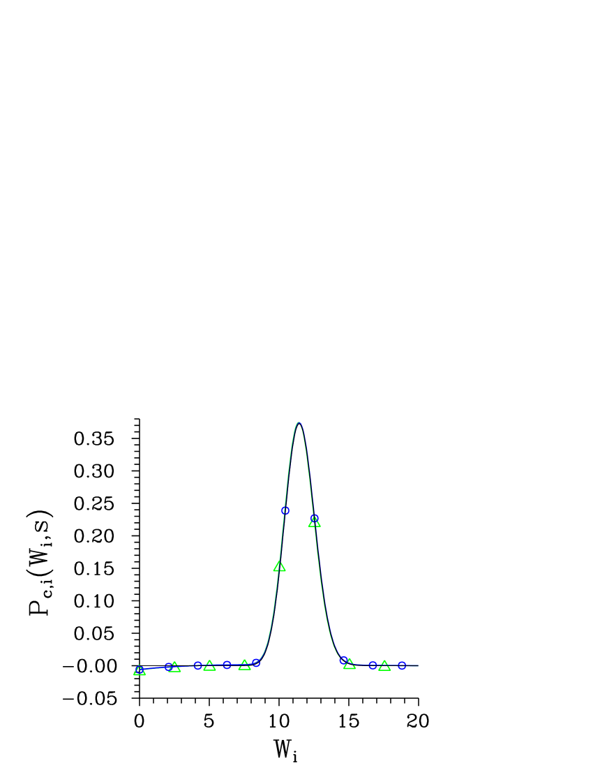
(a)                               (b)

Figure 8: Quasi-distributions $\tilde{P}_{\rm c,i}(W_{\rm i};s)$ of integrated intensity derived from those of the Poissonian field via Eq. (11) Perina1991 for (a) $s=0.9$ and (b) $s=0$ for the idler field post-selected by detection of $c_{\rm s}=5$ signal photocounts obtained by MLA (green curves with $\triangle$) and GTWB (blue curves with $\circ$); $\tau^{(2)}_{\rm i}\approx 0.14$. Distributions $\tilde{P}_{\rm Pois}$ of the corresponding Poissonian fields are drawn by plain curves for comparison.

In conclusion, we have shown that higher-order sub-Poissonian-like criteria based on intensity and photocount (photon-number) moments are suitable and comparably strong for revealing higher-order non-classicalities. Contrary to this, the criteria exploiting moments of intensity and photocount (photon-number) fluctuations have been found not very useful owing to their sensitivity to experimental errors. From the point of view of experimental errors, the criteria based on the elements of photocount distributions have been identified as the most powerful allowing us to experimentally reach even the ninth-order non-classicality.

References

- (1) A. Lukš, V. Peřinová, and J. Peřina. Principal squeezing of vacuum fluctuations. Opt. Commun., 67:149—151, 1988.
- (2) L. Davidovich. Sub-Poissonian processes in quantum optics. Rev. Mod. Phys., 68:127—173, 1996.
- (3) H. J. Kimble, M. Dagenais, and L. Mandel. Photon antibunching in resonance fluorescence. Phys. Rev. Lett., 39:691—694, 1977.
- (4) R. Short and L. Mandel. Observation of sub-Poissonian photon statistics. Phys. Rev. Lett., 51:384—387, 1983.
- (5) M. C. Teich and B. E. A. Saleh. Observation of sub-Poisson Franck-Hertz light at 253.7 nm. J. Opt. Soc. Am. B, 2:275—282, 1985.
- (6) P. R. Tapster, J. G. Rarity, and J. S. Satchell. Generation of sub-Poissonian light by high-efficiency light-emitting diodes. Europhys. Lett., 4:293—299, 1987.
- (7) R.-D. Li and P. Kumar. Quantum-noise reduction in travelling-wave second-harmonic generation. Phys. Rev. A, 49:2157—2166, 1994.
- (8) J. Bajer, O. Haderka, and J. Peřina. Sub-Poissonian behaviour in the second harmonic generation. J. Opt. B: Quantum Semiclass. Opt, 1:529—533, 1999.
- (9) R.-D. Li, S.-K. Choi, C. Kim, and P. Kumar. Generation of sub-Poissonian pulses of light. Phys. Rev. A, 51:R3429—R3432, 1995.
- (10) M. Koashi, K. Kono, T. Hirano, and M. Matsuoka. Photon antibunching in pulsed squeezed light generated via parametric amplification. Phys. Rev. Lett., 71:1164—1167, 1993.
- (11) J. Mertz, A. Heidmann, C. Fabre, E. Giacobino, and S. Reynaud. Observation of high-intensity sub-Poissonian light using an optical parametric oscillator. Phys. Rev. Lett., 64:2897—2900, 1990.
- (12) C. Kim and P. Kumar. Tunable sub-Poissonian light generation from a parametric amplifier using an intensity feedforward scheme. Phys. Rev. A, 45:5237—5242, 1992.
- (13) J. M. Raimond, M. Brune, and S. Haroche. Manipulating quantum entanglement with atoms and photons in a cavity. Rev. Mod. Phys., 73:565—583, 2001.
- (14) J.G. Rarity, P.R. Tapster, and E. Jakeman. Observation of sub-Poissonian light in parametric downconversion. Opt. Commun., 62:201—206, 1987.
- (15) J. Laurat, T. Coudreau, N. Treps, A. Maitre, and C. Fabre. Conditional preparation of a quantum state in the continuous variable regime: Generation of a sub-Poissonian state from twin beams. Phys. Rev. Lett., 91:213601, 2003.
- (16) H. Zou, S. Zhai, J. Guo, R. Yang, and J. Gao. Preparation and measurement of tunable highpower sub-Poissonian light using twin beams. Opt. Lett., 31:1735—1737, 2006.
- (17) M. Bondani, A. Allevi, G. Zambra, M. G. A. Paris, and A. Andreoni. Sub-shot-noise photon-number correlation in a mesoscopic twin beam of light. Phys. Rev. A, 76:013833, 2007.
- (18) J. Peřina Jr., O. Haderka, and V. Michálek. Sub-Poissonian-light generation by postselection from twin beams. Opt. Express, 21:19387—19394, 2013.
- (19) M. Lamperti, A. Allevi, M. Bondani, R. Machulka, V. Michálek, O. Haderka, and J. Peřina Jr. Optimal sub-Poissonian light generation from twin beams by photon-number resolving detectors. JOSA B, 31:20–25, 2014.
- (20) T. S. Iskhakov, V. C. Usenko, U. L. Andersen, R. Filip, M. V. Chekhova, and G. Leuchs. Heralded source of bright multi-mode mesoscopic sub-Poissonian light. Opt. Lett., 41:2149—2152, 2016.
- (21) G. Harder, T. J. Bartley, A. E. Lita, S. W. Nam, T. Gerrits, and C. Silberhorn. Single-mode parametric-down-conversion states with 50 photons as a source for mesoscopic quantum optics. Phys. Rev. Lett., 116:143601, 2016.
- (22) J. Peřina. Quantum Statistics of Linear and Nonlinear Optical Phenomena. Kluwer, Dordrecht, 1991.
- (23) B. E. A. Saleh. Photoelectron Statistics. Springer-Verlag, New York, 1978.
- (24) W. Vogel and D. G. Welsch. Quantum Optics, 3rd ed. Wiley-VCH, Weinheim, 2006.
- (25) R. J. Glauber. Coherent and incoherent states of the radiation field. Phys. Rev., 131:2766—2788, 1963.
- (26) E. C. G. Sudarshan. Equivalence of semiclassical and quantum mechanical descriptions of statistical light beams. Phys. Rev. Lett., 10:277—179, 1963.
- (27) C. T. Lee. Higher-order criteria for nonclassical effects in photon statistics. Phys. Rev. A, 41:1721—1723, 1990.
- (28) L. Mišta, V. Peřinová, J. Peřina, and Z. Braunerová. Quantum statistical properties of degenerate parametric amplification process. Acta Phys. Pol., A51:739—751, 1977.
- (29) C. K. Hong and L. Mandel. Higher-order squeezing of a quantum field. Phys. Rev. Lett., 54:323—325, 1985.
- (30) H. Prakash and D. K. Mishra. Higher order sub-Poissonian photon statistics and their use in detection of Hong and Mandel squeezing and amplitude-squared squeezing. J. Phys. B: At. Mol. Opt. Phys., 39:2291 –2297, 2006.
- (31) A. Verma and A. Pathak. Generalized structure of higher order nonclassicality. Phys. Lett. A, 374:1009—1020, 2010.
- (32) C. K. Hong and L. Mandel. Generation of higher-order squeezing of quantum electromagnetic fields. Phys. Rev. A, 32:974—982, 1985.
- (33) M. Hillery. Amplitude-squared squeezing of the electromagnetic field. Phys. Rev. A, 36:3796—3802, 1987.
- (34) M. Hillery. Squeezing of the square of the field amplitude in second harmonic generation. Opt. Commun., 62:135—138, 1987.
- (35) K. Kim. Higher order sub-Poissonian. Phys. Lett. A, 245:40—42, 1998.
- (36) D. N. Klyshko. Observable signs of nonclassical light. Phys. Lett. A, 213:7—15, 1996.
- (37) C. T. Lee. Simple criterion for nonclassical two-mode states. J. Opt. Soc. Am. B, 15:1187—1191, 1998.
- (38) I. I. Arkhipov, J. Peřina Jr., V. Michálek, and O. Haderka. Experimental detection of nonclassicality of single-mode fields via intensity moments. Opt. Express, 24:29496—29505, 2016.
- (39) C. T. Lee. Measure of the nonclassicality of nonclassical states. Phys. Rev. A, 44:R2775—R2778, 1991.
- (40) I. S. Gradshtein and I. M. Ryzhik. Table of Integrals, Series, and Products, 6th ed. Academic Press, San Diego, 2000.
- (41) J. Peřina Jr., M. Hamar, V. Michálek, and O. Haderka. Photon-number distributions of twin beams generated in spontaneous parametric down-conversion and measured by an intensified CCD camera. Phys. Rev. A, 85:023816, 2012.
- (42) J. Peřina Jr., O. Haderka, V. Michálek, and M. Hamar. State reconstruction of a multimode twin beam using photodetection. Phys. Rev. A, 87:022108, 2013.
- (43) J. Peřina Jr., O. Haderka, M. Hamar, and V. Michálek. Absolute detector calibration using twin beams. Opt. Lett., 37:2475—2477, 2012.
- (44) J. Peřina and J. Křepelka. Multimode description of spontaneous parametric down-conversion. J. Opt. B: Quant. Semiclass. Opt., 7:246—252, 2005.
- (45) A. P. Dempster, N. M. Laird, and D. B. Rubin. Maximum likelihood from incomplete data via the EM algorithm. J. R. Statist. Soc. B, 39:1—38, 1977.