NGC 307 and the Effects of Dark-Matter Haloes on Measuring Supermassive Black Holes in Disc Galaxies

Abstract

We present stellar-dynamical measurements of the central supermassive black hole (SMBH) in the S0 galaxy NGC 307, using adaptive-optics IFU data from VLT-SINFONI. We investigate the effects of including dark-matter haloes as well as multiple stellar components with different mass-to-light ($M/L$) ratios in the dynamical modeling. Models with no halo and a single stellar component yield a relatively poor fit with a low value for the SMBH mass ($7.0\pm 1.0\times 10^{7}M_{\sun}$) and a high stellar $M/L$ ratio ($\Upsilon_{K}=1.3\pm 0.1$). Adding a halo produces a much better fit, with a significantly larger SMBH mass ($2.0\pm 0.5\times 10^{8}M_{\sun}$) and a lower $M/L$ ratio ($\Upsilon_{K}=1.1\pm 0.1$). A model with no halo but with separate bulge and disc components produces a similarly good fit, with a slightly larger SMBH mass ($3.0\pm 0.5\times 10^{8}M_{\sun}$) and an identical $M/L$ ratio for the bulge component, though the disc $M/L$ ratio is biased high ($\Upsilon_{K,{\rm disc}}=1.9\pm 0.1$). Adding a halo to the two-stellar-component model results in a much more plausible disc $M/L$ ratio of $1.0\pm 0.1$, but has only a modest effect on the SMBH mass ($2.2\pm 0.6\times 10^{8}M_{\sun}$) and leaves the bulge $M/L$ ratio unchanged. This suggests that measuring SMBH masses in disc galaxies using just a single stellar component and no halo has the same drawbacks as it does for elliptical galaxies, but also that reasonably accurate SMBH masses and bulge $M/L$ ratios can be recovered (without the added computational expense of modeling haloes) by using separate bulge and disc components.

1 Introduction

The most commonly used technique for measuring the masses of supermassive black holes (SMBH) in galaxy centres is Schwarzschild modeling; fully two-thirds of the SMBH masses in the recent compilations of Kormendy & Ho (2013) and Saglia et al. (2016) were determined this way. Schwarzschild modeling entails the construction of gravitational potentials based on the combination of a central SMBH and one or more extended stellar components (which are typically based on deprojecting a 2D surface-brightness model of the galaxy in question), with the SMBH mass and stellar mass-to-light ($M/L$) ratio as variables. A library of stellar orbits is built up by integrating test particles within a given potential defined by particular values of SMBH mass and stellar $M/L$ ratio; these orbits are then individually weighted so as to reproduce the observed light distribution and stellar kinematics of the galaxy. The SMBH mass and stellar $M/L$ ratio are varied until the best match with the data is achieved.

Schwarzschild modeling has several advantages over methods based on modeling gas kinematics (the other major approach for measuring SMBH masses): it can be used in any galaxy bright enough for stellar kinematics to be measured, does not require the presence of gas, and does not require simplifying assumptions about the underlying kinematics (e.g., that all orbits are circular and coplanar).

Up until recently, the standard approach for Schwarzschild modeling of SMBH masses has been to treat galaxies as having just two components: a central SMBH and a stellar component with a single $M/L$ ratio. This is problematic for several reasons, the principal ones being that galaxies – especially disc galaxies – do not always have uniform $M/L$ ratios, and that galaxies have dark matter as well as stars.

Disc galaxies are widely recognized as having spatially varying stellar $M/L$ ratios, something at least partly due to different stellar populations in different subcomponents. Davies et al. (2006) introduced the idea of using two stellar components with distinct, independent $M/L$ ratios in order to model the combination of an actively star-forming nuclear star cluster within an older bulge in the spiral galaxy NGC 3227. Nowak et al. (2010) modeled the central bulges and main discs as separate stellar components for two spiral galaxies (NGC 3368 and NGC 3489); this was also done by Rusli et al. (2011) for the S0 galaxy NGC 1332. The modeling of separate $M/L$ ratios for bulges is also useful for investigating bulge-SMBH correlations, especially if one wants to determine bulge masses dynamically (e.g. Häring & Rix, 2004; Saglia et al., 2016).

Elliptical galaxies are in principle simpler to model than disc galaxies, because we can treat ellipticals as having a single stellar component (i.e., they can be approximated as pure “bulge” with no disc). However, they are known – like all galaxies – to possess haloes of dark matter. Recent work has focused on the question of whether the practice of ignoring these haloes in dynamical modeling might bias the resulting SMBH masses and stellar $M/L$ ratios. The key issue is whether the modeling process assigns extra mass to the stellar component in order to account for the (missing) effect of the halo. An increased stellar $M/L$ ratio can then result in a lower SMBH mass, because the stars at small radii will contribute more to the central potential than they would if the $M/L$ ratio were lower; this removes the need for a more massive SMBH.

Gebhardt & Thomas (2009) found that including a DM halo in their models for M87 resulted in a stellar $M/L$ ratio about half as large – and a SMBH mass about twice as large – as when their models included only a SMBH and the stellar component. Subsequent studies examining the inclusion of DM haloes in elliptical-galaxy models have yielded somewhat conflicting results, with some reporting effects similar to those found by Gebhardt & Thomas (2009) – e.g., McConnell et al. (2011) – and some reporting no differences between models with and without DM haloes – e.g., Shen & Gebhardt (2010); Jardel et al. (2011). Studies of larger samples by Schulze & Gebhardt (2011) and Rusli et al. (2013) have indicated that DM haloes can be safely ignored in the modeling only if high-spatial-resolution kinematics are available for the centre of the galaxy. Ideally, this means kinematic observations obtained with a point-spread-function whose FWHM is at least 5–10 times smaller than the diameter of the SMBH’s sphere of influence (Rusli et al., 2013).

What is not clear at this point is whether ignoring the existence of dark matter haloes in dynamical models of disc galaxies has any significant effect on either derived SMBH masses or bulge $M/L$ ratios. In this paper, we investigate this question by measuring the central SMBH mass and stellar $M/L$ ratios for the S0 galaxy NGC 307 using a four different models: first, a simple SMBH + single-stellar-component model; second, a model with a SMBH and two stellar components (bulge and disc) with separate $M/L$ ratios. We then add dark-matter haloes to both the single- and two-stellar-component models.

Unless otherwise specified, we adopt a cosmology where $\Omega_{m}=0.7$, $\Omega_{\Lambda}=0.3$, and $H_{0}=75$ km s^-1 kpc^-1.

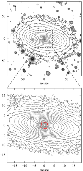
Figure 1: Top: Logarithmically scaled isophotes for the $R$-band WFI image of NGC 307 (smoothed with a 9-pixel-wide median filter). An elliptical disc embedded within a rounder and slightly skewed stellar halo can be seen. Bottom: Close-up of VLT-FORS1 $R$-band image (smoothed with a 3-pixel-wide median filter), showing the rounder bulge region within the disc. The small red square indicates the approximate field of view and orientation of our SINFONI observation.

2 NGC 307

NGC 307 is a poorly-studied early-type galaxy, classified as S$0^{0}$ by de Vaucouleurs et al. (1991). Although it lies only $\sim 0.5\degr$ from the centre of the cluster Abell 119, its much smaller redshift (0.0134 versus 0.044 for the cluster) means there is no physical association. In the group catalog of Garcia (1993), it is the second-brightest member of a small, five-galaxy group (LGG 13, brightest member = NGC 271). We adopt a distance of 52.8 Mpc, based on the (Virgocentric-infall-corrected) redshift of 3959 km s^-1 from HyperLEDA. Tonry & Davis (1981) reported a central velocity dispersion of $325\pm 15$ km s^-1, but more modern measurements indicate significantly lower values: $\sigma_{e}=239$ km s^-1 has been reported by van den Bosch et al. (2015), and Saglia et al. (2016) estimated $\sigma_{e}=205$ km s^-1, based on the kinematic and imaging data presented in this paper. Using the HyperLeda corrected $B\!-\!V$ colour (0.84) and the colour-based $M/L$ ratios of Bell et al. (2003) with either the HyperLeda $B_{\rm tc}$ magnitude (13.52) or the 2MASS total $H$ magnitude (9.865), we find estimated stellar masses of either $5.5\times 10^{10}M_{\sun}$ or $6.5\times 10^{10}M_{\sun}$, quite close to recent estimates of the Milky Way’s stellar mass (e.g., McMillan, 2011; Licquia & Newman, 2015; McMillan, 2017).

Figure 1 shows log-scaled $R$-band isophotes of NGC 307 using an image from the Wide Field Imager (WFI) on the ESO 2.2m telescope and a higher-resolution image from the FORS1 imager-spectrograph on the VLT; ellipse fits to both images are shown in Figure 2 (see Section 3.3 for more about the images). These fits show a fairly broad peak in isophotal ellipticity of $\epsilon\approx 0.65$ extending from semi-major axis $a\sim 20\arcsec$ to $a\sim 40\arcsec$, with the isophotes becoming significantly rounder (as low as $\sim 0.30$) further out. This suggests that we may be seeing a disc embedded within a rounder, luminous halo (we will show in Section 6.2 that the latter is unlikely to be just an extension of the central bulge). In addition, unsharp masks suggest the existence of a weak bar or lens within the disc, with semi-major axis $\sim 10\arcsec$; this matches the shoulder in ellipticity seen in the ellipse fits and the corresponding slight twist in the position angle to a local minimum of $\sim 81\degr$ at $\approx 9$–10″.

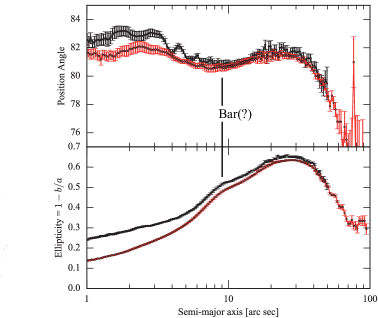
Figure 2: Position angles and ellipticities from ellipse fits to the WFI (red) and VLT-FORS1 (black) $R$-band images of NGC 307. The label indicates the position-angle twist and local shoulder in the ellipticity profile corresponding to a possible bar or lens.

3 Observations

3.1 Spectroscopy: SINFONI IFU Data

Our primary set of spectroscopic data comes from observations made at the VLT with SINFONI in November of 2008. SINFONI combines the near-IR integral field spectrograph SPIFFI and the adaptive-optical module MACAO (Eisenhauer et al., 2003; Bonnet et al., 2004), using an image-slicer to subdivide the field of view into 32 slitlets, which are subsequently rearranged into a composite pseudo-long-slit image that is passed into the main spectrograph. After dispersion by the grating, the resulting composite spectrum is imaged onto a $2048\times 2048$ Hawaii 2RG detector.

The pre-optics of SINFONI allow the user to select one of three different spatial resolution modes: 25, 100, or 250 mas, corresponding to fields of view of $0.8\arcsec\times 0.8\arcsec$, $3\arcsec\times 3\arcsec$, or $8\arcsec\times 8\arcsec$. For NGC 307, we used only the middle (100mas) scale, along with the $K$-band grating, since our primary target was the CO absorption bandheads at $2.3$ µm. A single exposure, when assembled into a datacube, yields rectangular spatial elements with sizes of $50\times 100$ mas for the 100 mas mode; when multiple exposures with appropriate dithering are combined, the resulting datacubes have a spatial pixel scale of 50 mas pixel^-1. The resulting $K$-band velocity resolution is $\sigma=53$ km s^-1.

Since NGC 307 is much larger than the SINFONI field of view, we observed it using a sequence of multiple ten-minute exposures organized into an object-sky-object pattern; the sky exposures were made with an offset of 80″ along the galaxy minor axis to avoid contamination by galaxy light. Individual ten-minute exposures were dithered using offsets of a few (spatial) pixels, to reduce the effects of bad pixels in the detector and to allow construction of a final data cube with full spatial resolution. The complete set of observations included 40 minutes of on-target time on each of two night – 2008 November 25 and 26 – for a total of 80 minutes integration time. However, we found the observations from the first night to be of significantly higher quality in terms of AO performance and achieved resolution; since they had sufficient S/N by themselves, we only used that night’s data. Observations of telluric-standard B stars, obtained immediately after the galaxy observations and at similar air masses, were used to remove atmospheric absorption (see below).

The centre of NGC 307 was not bright enough to serve as an AO guide source by itself, so we used the PARSEC laser guide star (LGS) system at the VLT (Bonaccini et al., 2002; Rabien et al., 2004). The LGS mode still requires an extra-atmospheric reference source for “tip-tilt” correction of lower-order atmospheric distortions; we used the galaxy nucleus for this.

Data reduction was performed using a custom-built pipeline combining the official ESO SINFONI Pipeline (Modigliani et al., 2007) with elements from its predecessor, the SPIFFI Data Reduction Software (SPRED; Schreiber et al., 2004; Abuter et al., 2006). This combined pipeline included the standard bias-correction, dark subtraction, distortion correction, non-linearity correction, flat-fielding, wavelength calibration, and datacube generation stages. Sky subtraction, which used the sky datacube observed closest in time for each galaxy datacube, was augmented using the IDL code of Davies (2007) to account for variations in night-sky emission-line strengths between the times of the galaxy and sky observations.

The galaxy datacubes were then corrected for telluric absorption using the telluric-star datacubes. This involved extracting a single, summed spectrum for the telluric star from its datacube and then dividing it by a blackbody curve with a temperature appropriate for the spectral type of the star (the Paschen $\gamma$ absorption line in the standard-star spectrum was fit by hand using code written in IDL). The resulting normalized spectrum was then used to correct the individual spectra in the corresponding galaxy datacubes. Finally, the individual datacubes were combined into a single datacube for the night, taking into account the recorded dither positions in the headers.

To estimate the resolution obtained by the LGS system, we used “PSF star” observations obtained during or immediately after the galaxy observations, with exactly the same instrument setup and AO mode (i.e., LGS). To make the match as close as possible, the PSF stars were chosen to have the same $R$-band magnitude and $B-R$ colour as the galaxy nucleus (measured within a 3″-diameter aperture), so that the AO system would respond in a similar fashion. Although it is always possible that the PSF star measurements reflect different observing conditions, Hicks et al. (2013) reported that measurements of PSF stars taken after their (non-AO) VLT-SINFONI observations showed FWHM agreement to within 0.02″ for galaxies with bright AGN, where the AGN itself could be used to independently measure the seeing. The combined PSF-star datacube was flattened to produce a $K$-band image, which was then fit with the sum of two Gaussians using Imfit (Erwin, 2015). The inner Gaussian component (37% of the total light), which was mildly elliptical, had FWHM measured along its major and minor axes of 0.20″ and 0.16″, respectively, for a mean resolution of 0.18″. The outer component was nearly circular, with a FWHM of 0.48″. This PSF is consistent with previously published SINFONI 100mas K-band values when using the laser guide star; in fact, it is equal to the median value from our previously published observations with the LGS in the same mode (Nowak et al., 2010; Rusli et al., 2013; Mazzalay et al., 2013).

3.2 Spectroscopy: VLT/FORS1 and VIRUS-W Observations

To obtain measurements of the stellar kinematics outside the central $3\arcsec\times 3\arcsec$ field of view provided by our SINFONI data, we made two sets of optical spectroscopic measurements: long-slit observations along the galaxy major and minor axes with the FORS1 spectrograph in the VLT, and wide-field IFU observations with the VIRUS-W spectrograph on the McDonald 2.7m telescope.

3.2.1 VLT/FORS1

We obtained long-slit data along the galaxy major and minor axes with the VLT-FORS1 spectrograph on 2008 October 23 (Programme ID 082.A-0270). We made a total of four 2700s exposures with the slit oriented along the galaxy major axis (PA = 78.1°) and two more exposures of the same integration time with the slit along the minor axis (PA = 168.1°). The instrument was used with the 1200g grism and a slit width of 1.6″ width slit; the instrumental dispersion was $\sigma\approx 79$ km s^-1.

The reduction of the FORS1 spectra followed the standard steps of bias subtraction, flat fielding, cosmic-ray rejection, and wavelength calibration to a logarithmic scale using our customized MIDAS scripts (de Lorenzi et al., 2008). We subtracted the sky measured at the ends of the slit and binned the resulting frame radially to obtain a set of spectra with approximatly the same signal to noise ratios.

The kinematic analysis of the spectra is discussed in in Section 4.2, and our stellar-population analysis is discussed in Section 5.

3.2.2 VIRUS-W

VIRUS-W is an optical integral-field-unit spectrograph with a $105\arcsec\times 55\arcsec$ field of view, based on the VIRUS IFU design for HETDEX (Hoby-Eberly Telescope Dark Energy Experiment) and adapted to achieve high spectral resolution for deriving stellar kinematics (Fabricius et al., 2012). It has 267 fibers with core diameters of 3.14″ on the sky, arranged in a rectangular array with a fill factor of one-third.

We observed NGC 307 with VIRUS-W mounted on the 2.7m Harlan J. Smith telescope at the McDonald Observatory in Texas on 2010 December 6, as part of commissioning/science-verification time for the instrument. The galaxy was observed using a total of three dither positions (to account for the 1/3 fill factor), each with 1200s exposure time. These were bracketed and interleaved with sky offset exposures, also using 1200s exposure times. The seeing varied in FWHM from 1.2″ to 1.9″. VIRUS-W has both low- and high-resolution spectral modes; although we observed NGC 307 with both modes, we ended up using just the low-resolution mode data. Since the low-resolution mode has $\sigma_{\rm instr}=39$ km s^-1 ($R=3300$, with a spectral coverage of 4320–6042 Å), it provided more than sufficient spectral resolution for NGC 307.

Data reduction used a custom pipeline based on the Cure pipeline for for HETDEX; see Fabricius et al. (2014) for details. The result is a datacube with $1.6\times 1.6\arcsec$ spaxels.

In order to generate high-$S/N$ spectra for kinematic extraction, we combined spectra from individual spaxels using the Voronoi binning scheme of Cappellari & Copin (2003), ending up with a median $S/N$ per bin of 29. The kinematic analysis of the binned spectra is discussed in in Section 4.2.

3.3 Imaging Data

The available imaging data for NGC 307 consist of a large-scale $R$-band image from a 300s exposure at the ESO-MPI 2.2m Wide Field Imager on 2010 July 15 (Programme ID 084.A-9002), with seeing FWHM $=1.62\arcsec$; a 10s-exposure VLT-FORS1 image with smaller field of view (also $R$-band, with FWHM = 1.00″) made during our spectroscopic observations with FORS1 (above); and our VLT-SINFONI combined datacube, collapsed along the wavelength axis to form a $\sim 3\arcsec\times 3\arcsec$ $K$-band image.

These images are, to a degree, complementary: the WFI image is wide enough and deep enough to allow determination of the outer stellar halo and main disc, but has relatively poor resolution; the FORS1 image provides better resolution for the bar/lens and the disc-bulge transition region, but is not as good for characterizing the halo due to its smaller field of view, lower S/N, and the fact that the outer part of the galaxy falls on an inter-chip gap; and the SINFONI image has the best resolution for the inner region of the bulge. Consequently, we construct our final photometric models using a combination of all three images.

Since the innermost data are $K$-band, we calibrated all three images to $K$-band by a multi-step process similar to that used by Nowak et al. (2010); the resulting calibration is ultimately based on the publicly available 2MASS $K$-band image of the galaxy. First, we calibrated the FORS1 image by convolving it to the resolution of the 2MASS image and performing aperture photometry on both images. We then calibrated the SINFONI $K$-band image to the FORS1 image by iteratively matching surface-brightness profiles from ellipse fits to both images in the region $a=0.6$–1.42″, including a sky-background term for the SINFONI data. Finally, the WFI image was calibrated to match the $K$-band-calibrated FORS1 image using a similar ellipse-fit profile-matching technique for the region $a=15$–45″.

4 Stellar Kinematics

4.1 SINFONI Kinematics

For our SINFONI data, we extracted full, non-parametric line-of-sight velocity distributions (LOSVDs) from the spectra, using a total of 21 bins in velocity space. We used a maximum penalized likelihood (MPL) method originally introduced by Gebhardt et al. (2000) and a set of stellar template spectra of K and M giants derived from earlier SINFONI observations with the same instrumental setup (see, e.g. Nowak et al., 2007, 2008, 2010).

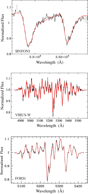
Figure 3: Examples of kinematic fits to our spectroscopy. Top: best-fit, LOSVD-convolved model spectrum (red) and binned VLT-SINFONI data from one of the central bins (black line); dashed lines indicate regions of the spectrum not used in the fit. The observed spectrum has been normalized by division by a smooth continuum fit. Middle: Best-fit model spectrum (red) and observed optical spectrum (black) from the central bin of the VIRUS-W observations; the observed spectrum has been normalized by subtracting a smooth continuum fit. Bottom: Same, but now for the FORS1 major-axis spectrum.

We focused on the spectral region containing the first two CO bandheads ¹²CO(2–0) and ¹²CO(3–1), which corresponds to a rest-frame spectral range of 2.279–2.340 µm. In order to minimize template mismatch, we limited our set of template stars to those with equivalent widths for the first CO bandhead which were similar to the equivalent width of the galaxy spectra (Silge & Gebhardt, 2003). A trial LOSVD was convolved with a linear combination of template spectra, and the resulting model spectrum was compared with the data. The LOSVD and the weights for the template spectra were adjusted by minimizing a penalized $\chi^{2}$ function:

$$\chi^{2}_{\rm P}\;=\;\chi^{2}\,+\,\alpha\mathcal{P},$$ (1)

where $\mathcal{P}$ is the penalty function (the integral of squared second derivative of the LOSVD) and $\alpha$ is a smoothing parameter. The appropriate value of $\alpha$ depends on the S/N of the data and the velocity dispersion of the galaxy; our choice was based on extensive simulations involving MPL fitting of template stellar spectra convolved with different LOSVDs; see Nowak et al. (2008) for more details. An example of one of our fits is shown in the upper panel of Figure 3.

To increase the S/N of the spectra, we binned individual spaxels into angular and radial bins using luminosity-weighted averaging. This involved dividing the galaxy into four quadrants; the boundaries of the quadrants were set by the major and minor axes of the galaxy. Each quadrant was subdivided into five angular bins and seven radial bins. (See Figure 4 for the binning, and the first panel for definitions of the quadrants.)

Uncertainties for the best-fitting LOSVDs were determined by a Monte Carlo technique, where for each spectrum we created 100 realizations of the best-fitting combined template spectrum, convolved with the best-fitting LOSVD, and then added Gaussian noise based on the measured RMS deviations of the original fit. Each such spectrum was then fit using the same MPL approach, with the final uncertainties based on the distribution of fitted LOSVDs from the Monte Carlo realizations.

For presentation purposes, we parameterized the LOSVDs using the Gauss-Hermite moments (Gerhard, 1993; van der Marel & Franx, 1993) velocity $v$, velocity dispersion $\sigma$, $h_{3}$, and $h_{4}$. Maps of these four moments are shown in Figure 4. Significant rotation can be seen in the velocity field, with an accompanying anti-correlation in the $h_{3}$ values. A somewhat noisy trend of increasing velocity dispersion towards the galaxy centre can also be seen. No trends are visible in the $h_{4}$ map.

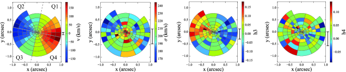
Figure 4: Stellar kinematics (from left to right: velocity, velocity dispersion, $h_{3}$, and $h_{4}$) from our VLT-SINFONI observations of NGC 307, using our radial and angular binning scheme. Note that our dynamical modeling uses the full LOSVD from each bin, not the Gauss-Hermite moments we show in this figure. Maps have been rotated so that north is up and east is to the left. Solid and dashed grey lines in the first panel indicate galaxy major and minor axes, respectively; “Q1” through “Q4” labels indicate Quadrants 1 through 4, as used in our dynamical modeling. Error bars next to the colour bars indicate median errors from Monte Carlo simulations.

4.2 Optical Kinematics

Stellar kinematics for both the VLT-FORS1 long-slit spectra and the Voronoi-binned VIRUS-W spectra were derived using the Fourier Correlation Quotient (FCQ) method (Bender, 1990; Bender et al., 1994), which models the LOSVD using a Gauss-Hermite decomposition, producing stellar velocity $V$ and velocity dispersion $\sigma$ values, along with $h_{3}$ (skew) and $h_{4}$ (kurtosis) deviations from Gaussianity. The FORS1 kinematics were measured as done in Saglia et al. (2010), chosing the best-fitting template from the simple stellar population model spectra of Vazdekis (1999). For the VIRUS-W data, we used a single K2 III template star (HR 2600) spectrum previously observed with VIRUS-W, using a rest-frame spectral range of 4537–5442 Å and removing the continuum using an eight-order polynomial. Error estimates for the $V$, $\sigma$, $h_{3}$, and $h_{4}$ measurements in both cases were obtained using a Monte Carlo approach (Mehlert et al., 2000). Examples of individual fits are shown in the middle and lower panels of Figure 3.

Figures 5 and 6 show the major- and minor-axis stellar kinematics from the FORS1 spectra, and Figure 7 shows the kinematic maps for the VIRUS-W data. Figure 8 compares stellar kinematics extracted along the major axis from our three datasets. Given the differences in the resolution for the different observations (the respective FWHM or fiber sizes are indicated by vertical shaded regions in the figures) – and the relative noisiness of the higher-order $h_{3}$ and $h_{4}$ moments – the overall agreement between the three datasets is good.

Both the major- and minor-axis long-slit kinematics show that the velocity dispersion rises quite steeply in the inner $r\la 5\arcsec$, suggestive of a kinematically hot central component. This can also be seen, less clearly, in the higher dispersion of the central three bins of the VIRUS-W data. There is, non the less, evidence for significant rotation as in this region as well, as can be seen in the strong inner velocity peak at $r\sim 3\arcsec$ and accompanying $V$–$h_{3}$ anti-correlation in the major-axis kinematics (Figure 5). Outside this region, the kinematics are strongly rotation-dominated, with an observed peak velocity of $\sim 200$ km s^-1 and a dispersion profile that declines to below 100 km s^-1 for $r\ga 20\arcsec$ along the major axis.

As a whole, then, the stellar kinematics suggest a kinematically hot central region (e.g., a classical bulge, albeit one with significant rotation, or possibly a fast-rotating subcomponent) within the central 5″ and a dominant disc component at larger radii. As we will show below, this is consistent with both our stellar population analysis of the FORS1 spectra and with our morphological analysis and 2D decomposition of the galaxy.

There is photometric evidence for a weak bar or lens in NGC 307, extending to about 10″ in radius (see Sections 2 and 6.2). Is there any evidence for this bar in the stellar kinematics? We compare the observed kinematics with predictions from $N$-body models published by Bureau & Athanassoula (2005) and Iannuzzi & Athanassoula (2015), paying particular attention to projections where the bar orientation is similar to that in NGC 307 (i.e., with the bar viewed nearly side-on). Although some of the $N$-body model projections show a “double-hump” major-axis velocity profile, which might seem to agree with the clear double-peak in NGC 307’s velocity profile (upper left panel of Figure 5), this feature is only visible in the models when the bar is close to end-on, and vanishes when the bar is closer to side-on. The double-hump velocity feature in NGC 307 is thus almost certainly not a bar signature; it is more likely due to a rapidly rotating substructure within the classical bulge region.

The models do predict local extrema in $h_{3}$ – and maxima in $h_{4}$ – near the ends of a strong bar seen side-on and at inclinations of $75$ or 80° (e.g., lower right subpanels of Fig. 4 in Bureau & Athanassoula 2005). While there are local extrema in NGC 307’s $h_{3}$ profile at $r\sim 6$″which might be consistent with this prediction, there are no such features in the $h_{4}$ profile (Figure 5). We conclude that there is no evidence that the bar/lens strongly affects the stellar kinematics in this galaxy.

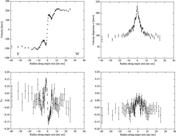
Figure 5: Major-axis (PA $=78.1\degr$) stellar kinematics from our VLT-FORS1 observations of NGC 307.

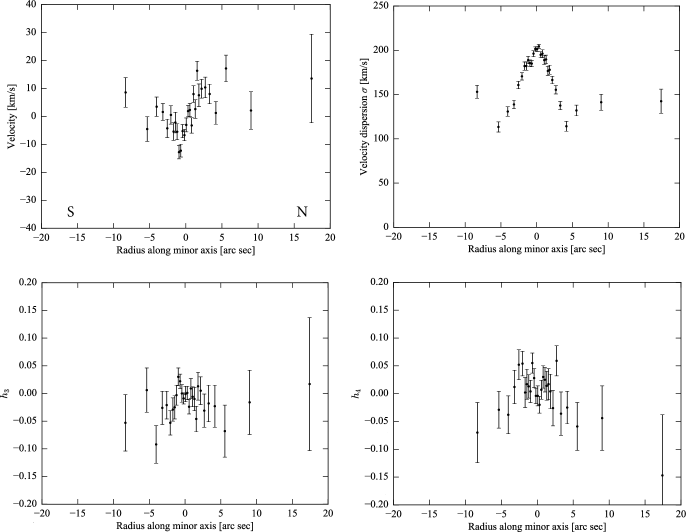
Figure 6: Minor-axis (PA $=168.1\degr$) stellar kinematics from our VLT-FORS1 observations of NGC 307.

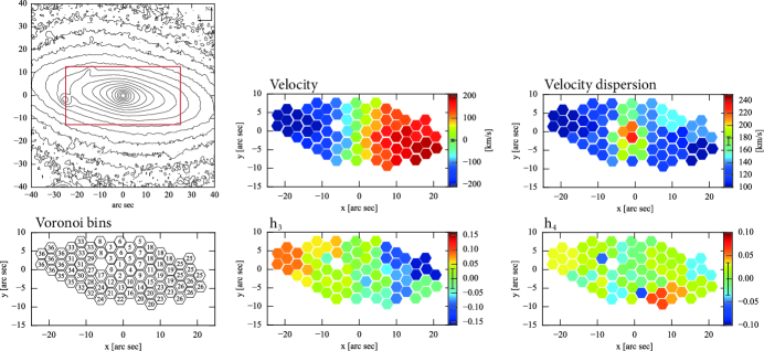
Figure 7: Stellar kinematics from our VIRUS-W observations of NGC 307. Upper left: $R$-band contours for NGC 307 from WFI image (median-smoothed with width = 5 pixels); the red box corresponds to the sizes of the other panels. Lower left: Map of fiber positions; numbers indicate which Voronoi bins individual fibers belong to. Middle and right: Stellar kinematic maps ($V$, $\sigma$, $h_{3}$, $h_{4}$). Error bars inside the colour bars indicate median errors from Monte Carlo simulations.

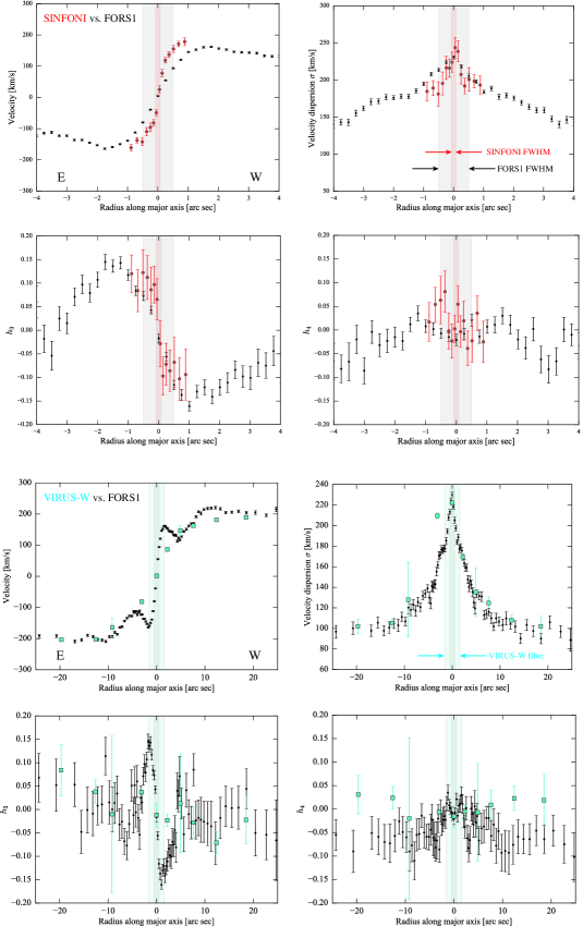
Figure 8: Comparison of major-axis stellar kinematics from our SINFONI (medium-sized red circles), VLT-FORS1 (small black circles), and VIRUS-W (cyan squares) observations of NGC 307. The FWHM or fiber sizes of the observations are indicated by the vertical shaded regions.

4.3 Quadrants for Stellar Kinematics

As noted above (Section 4.1), the SINFONI kinematics were derived using a radial-angular binning scheme, with the galaxy divided into four quadrants whose boundaries were the major and minor axes of the galaxy. Each quadrant was subdivided into five angular bins of varying width, with seven radial bins spaced logarithmically out to the edge of the SINFONI field of view (Figure 4). To include the optical kinematics in the same scheme for our dynamical modeling, we extended the quadrants with additional radial bins and assigned values from the optical kinematics.

Since the FORS1 long-slit orientations were along the quadrant boundaries, we assigned their kinematic values to the corresponding bins along the quadrant boundaries – e.g., the major-axis data were assigned to corresponding closest bins along the major-axis boundaries of the quadrants. For the Voronoi-binned VIRUS-W kinematics, we assigned each Voronoi bin’s kinematic values to the radial-angular bin containing the center of the Voronoi bin.

5 Stellar Population Analysis

To get a preliminary sense of how stellar populations – and thus $M/L$ ratios – might vary within NGC 307, we performed a stellar-population analysis of our FORS1 long-slit spectroscopy.

We measured the Lick line strength index profiles from H$\beta$ to Fe5406 as in Mehlert et al. (2000). Following the minimum $\chi^{2}$ procedure described in Saglia et al. (2010), we determined the age, metallicity, and [$\alpha/$Fe] overabundance profiles that best reproduced the observed profiles of the Lick indices H$\beta$, Mg$b$, Fe5015, Fe5270, Fe5335, and Fe5406 using the simple stellar population (SSP) models of Maraston (1998, 2005), with a Kroupa (2001) IMF and the modeling of the Lick indices with $\alpha$-element overabundance of Thomas et al. (2003). We are able to reproduce the Mg and Fe indices quite well; however, the measured H$\beta$ is systematically $\approx 0.2$ Å smaller than the models. As a consequence of this, the resulting ages hit the maximum allowed value (15 Gyr) of the model grid for most of the cases. The [$\alpha/$Fe] profile is approximately flat at a level of +0.3 dex, on both the major and minor axes.

Figure 9 show some of the results, including both raw Mgb and Fe5270 index measurements and the overall metallicity ([Z/H]) and $K$-band stellar $M/L$ ratio estimates. The metallicity is slightly above the solar value in the inner $r\la 5\arcsec$ and drops to half-solar outside. The $K$-band $M/L$ ratio implied by the derived age and metallicity profiles is approximately constant at a value of 1.22 $M_{\odot}/L_{\odot}$ at radii $\ga 10\arcsec$, rising to a central peak of $\sim 1.26$. Actual radial variations in the $M/L$ ratio are probably underestimated due to the saturated SSP age estimates.

Both major- and minor-axis profiles show evidence for a central peak in metallicity, with a correspondingly higher $M/L$ ratio. This is good evidence for a separate, metal-rich population with a higher $M/L$ ratio dominating the inner $r\la 5\arcsec$ along the major axis. As noted above, our VLT-FORS1 kinematics (Figure 5 and 6) show that the stellar velocity dispersion increases rapidly towards the centre in this same region, from a nearly constant disc value of $\sim 110$–120 km s^-1 to values $>200$ km s^-1, suggesting a classical, dispersion-dominated (albeit rapidly rotating) bulge. This is also consistent with the decompositions we perform (below), which argue for a relatively round luminosity component dominating the light at $r\la 5\arcsec$, and motivates separating out the bulge component and allowing it to have its own $M/L$ ratio in the modeling process.

Figure 9: Stellar-population analysis of VLT-FORS1 long-slit spectrum of NGC 307, showing major-axis (left panels) and minor-axis (right panels) results. In each set of panels, the left-hand two panels show examples of measured absorption-line indices (top: Mgb; bottom: Fe5270); the right-hand two panels show results of the analysis (top: best-fitting SSP metallicity; bottom: best-fitting SSP $K$-band $M/L$ ratio, assuming a Kroupa IMF). Both major- and minor-axis profiles show a strong central increase in stellar metallicity, and a weaker increase in the $M/L$ ratio. We associate both with the dominance of a distinct “classical bulge” component in the inner $r\la 5\arcsec$, also seen in the stellar kinematics and morphology.

6 Photometric Modeling

6.1 General Approaches

To properly measure the mass of a galaxy’s SMBH, we must construct a dynamical model based on at least two components: the potential of the central SMBH and the potential due to the stellar mass distribution. (In some cases, gas may also form a significant component; however, in Mazzalay et al. 2013, we presented evidence that the molecular gas content in the centres of the disc galaxies we observed with SINFONI – that is, those galaxies where we could detect gas – was much lower than the stellar mass in the same region, and so could reasonably be neglected. In the case of NGC 307, we detected no gas emission at all; an absence of significant gas is consistent with its S0 classification and the lack of visible dust lanes in the optical images.) The stellar-mass potential is the combination of a stellar $M/L$ ratio – something adjusted during the fitting process – and a luminosity-density model for the stellar light. The luminosity-density model, in turn, is derived from the observed stellar light distribution of the galaxy, usually by deprojecting an observed surface-brightness model. In this section, we describe how we devise luminosity-density models for NGC 307.

The standard approach for constructing luminosity-density models has been to fit ellipses to the isophotes of a galaxy image, and use the resulting ellipse-fit model – i.e., surface brightness, ellipticity, and possibly symmetric higher-order terms ($\cos 4\theta$, $\cos 6\theta$, etc.) as a function of semimajor axis – as input to the code which then deprojects this to obtain a 3D luminosity-density model. An alternate approach is to model the isophotes as the sum of multiple 2D Gaussians, which can then be deprojected individually and summed to form the luminosity density model (Emsellem et al., 1994; Cappellari, 2002). In the case of something simple like most elliptical galaxies, this is usually a straightforward operation, since we can assume that the entire galaxy is a single, coherent stellar component.

But in constructing photometric models of disc galaxies, we face two problems. The first has to do with questions of stellar $M/L$ ratios. As noted above, most Schwarzschild modeling in the past has assumed a single $M/L$ ratio for the entire stellar component. While this is perhaps reasonable for elliptical galaxies, disc galaxies are known to contain multiple stellar populations which can dominate different regions of a galaxy. In the simplest case, a disc galaxy may have distinct populations belonging to the bulge and to the disc; our spectroscopic analysis suggests this is indeed the case for NGC 307 (Section 5).

One possible approach is to consider a $M/L$ ratio which varies as a simple function of radius (McConnell et al., 2013). But this may or may not have a plausible physical origin, and there are a potentially unlimited number of possible radial profiles to choose from, with varying numbers of additional free parameters; even a linear function adds two extra free parameters to the modeling process. We choose instead a somewhat more physically motivated approach: we assume that the galaxy can be spatially decomposed into two or more overlapping but distinct stellar components, each with its own $M/L$ ratio (Davies et al., 2006; Nowak et al., 2010; Rusli et al., 2011).

The second problem we have when constructing photometric models stems from the fact that our Schwarzschild modeling code assumes an axisymmetric stellar potential, which can be described as a set of coplanar, axisymmetric spheroids with relative thicknesses which can vary as a function of radius (i.e., spheroids with $a=b$ but varying vertical scale heights $c$). This requires an axisymmetric photometric model as input to the deprojection algorithm: the isophote shapes can vary (in ellipticity and higher-order moments), but their orientations (position angles) cannot. Real disc galaxies, however, are often non-axisymmetric, with bars, spiral arms, and other stellar substructure which show up in ellipse fits as variations in ellipticity and position angle. Since the deprojection process cannot handle position-angle variations, they are ignored, and the result is that changes in isophotal ellipticity due to, e.g., bars or spiral arms are misleadingly converted into changes in vertical thickness in the resulting luminosity-density model.

To deal with these issues, we use an approach first described in Nowak et al. (2010) and applied to the galaxies NGC 3368 and NGC 3489 in that paper, and also to NGC 1332 in Rusli et al. (2011). This consists of first identifying plausible “bulge” and “disc” regions, devising preliminary models corresponding to the bulge and disc, creating separate residual images for the two components (i.e., a “bulge-only” image which has the disc model subtracted off and a “disc-only” image with the bulge model subtracted off), and then treating them in distinct fashions:

1. The bulge-only residual image is fit with freely varying ellipses in the standard fashion, treating it as though it were the image of a spheroidal, axisymmetric structure with potentially variable $c/a$ axis ratios.

2. The disc-only residual image is fit with ellipses which are fixed to a common shape and orientation (axis ratio and position angle) corresponding to that of the outer disc. This has the effect of azimuthally averaging whatever non-axisymmetric structure – bars, spiral arms, etc. – may actually exist.

Although we generate preliminary models for both bulge and disc based on combinations of simple analytic components (e.g., an elliptical Sérsic component for the bulge), the final surface-brightness models which we pass to the deprojection machinery are based primarily on direct ellipse fits to the residual images as outlined above. This means that the final models – especially for the bulge component – contain as much of the intrinsic galaxy light variation as possible: e.g., our final bulge component is not a pure Sérsic component, but represents the galaxy light after the preliminary disc model has been subtracted.

In the specific case of NGC 307, as we will discuss below, there is evidence for a rounder stellar “halo” which dominates the light beyond a certain radius. Thus, we modify the second surface-brightness component described above by allowing the isophotes to have lower ellipticities (as measured by ellipse fits with variable ellipticity) at large radii.

6.2 Photometric Modeling of NGC 307

As noted above, there is evidence for a central bulge in NGC 307 with a distinct metal-rich stellar population dominating the inner $r\la 5\arcsec$, a weak bar or lens contributing to the light at intermediate radii (most strongly at $r\sim 9$–10″), and a halo dominating the outer light ($r\ga 50\arcsec$). Therefore, we analysed this galaxy with a 2D decomposition approach, including up to four components: central bulge, bar/lens, disc, and halo. (Note that in this subsection we use “halo” to refer specifically to a stellar component, not to a dark-matter halo.)

To start with, we fit the FORS1 image with Imfit (Erwin, 2015) using several models, including both a simple bulge + disc (B+D = Sérsic + exponential) model and two versions of a bulge + bar/lens + disc (B+b+D) model, which differed in how the bar/lens was modeled. A Moffat PSF based on the median values of fits to stars in the image was convolved with each model during the fitting process. We compared the effectiveness of the models using the Akaike Information Criterion (AIC; Akaike, 1974), which is automatically computed by Imfit based on the likelihood of the best-fitting model, the number of data points, and the number of parameters. Lower values of AIC indicated (relatively) better fits. A difference in AIC values between two models of $<2$ is considered insignificant, while a difference $>6$ is considered strong evidence for the model with lower AIC being better.

The best of these models, with the lowest AIC, was the B+b+D model with the bar/lens represented by an elliptical, broken-exponential component (Erwin et al., 2008; Erwin, 2015). Using a Sérsic function for the bar/lens provided a reasonable fit, though not nearly as good ($\Delta$AIC = +675 relative to the broken-exponential model). The baseline B+D model was a much poorer fit, with $\Delta$AIC = +4291 relative to the broken-exponential model.

To determine the contribution of the halo component, we then performed a four-component (B+b+D+H) fit to the (larger FOV) WFI image, starting with the best B+b+D model from the FORS1 image fits and adding a Sérsic component with generalized ellipses (i.e., boxy or discy isophote shapes) to represent the halo. Generalized ellipses are described by

$$\left(\frac{|x|}{a}\right)^{c_{0}\,+\,2}\!\!+\;\left(\frac{|y|}{b}\right)^{c_{0}\,+\,2}=\;1,$$ (2)

where $|x|$ and $|y|$ are distances from the ellipse centre in the coordinate system aligned with the ellipse major axis, $a$ and $b$ are the semi-major and semi-minor axes, and $c_{0}$ describes the shape: $c_{0}<0$ corresponds to disky isophotes, $c_{0}>0$ to boxy isophotes, and $c_{0}=0$ for perfect ellipses. The best-fitting halo component had slightly boxy isophotes ($c_{0}=0.57$) and a profile essentially indistinguishable from an exponential (Sérsic $n=0.97$); this component is slightly misaligned with respect to the disc and bulge (both disc and bulge have PA $\approx 82\degr$, while the halo has PA $\approx 77\degr$). We then re-fit the (higher-resolution) FORS1 image by including the halo component, keeping most of its structural parameters fixed to the best-fitting values from the WFI fit but allowing the position angle and intensity ($I_{e}$) to be free parameters.

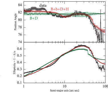
Figure 11: Position angles and ellipticities from ellipse fits to the VLT-FORS1 and WFI images of NGC 307 (black, using FORS1 data for $a<46\arcsec$), the best-fitting, PSF-convolved 2D bulge + disc model image (B+D, green), and the best-fitting, PSF-convolved 2D bulge + bar + disc + outer halo model image (B+b+D+H, red). The latter model is significantly better at reproducing the isophote shapes.

Figure 10 compares our final four-component B+b+D+H fit to the FORS1 image (lower panels) with the baseline B+D fit (upper panels); the parameters of the B+b+D+H fit are listed in Table 1. In addition to the fact that the second decomposition is a significantly better fit in a statistical sense (e.g., $\Delta$AIC is $-5486$ relative to the B+D model, and $-1491$ relative to the best B+b+D model), we can see that the B+D fit has an exceptionally narrow disc (ellipticity = 0.80) and an exceptionally bright bulge component with Sérsic index $n=5.5$; the value of $n=2.5$ for the bulge in the B+b+D+H fit is much more typical of bulges in S0 galaxies (Laurikainen et al., 2010). Figure 11 compares ellipse fits to the data (black) and to the B+D (green) and B+b+D+H (red) model images; the latter does a significantly better (albeit not perfect) job of matching position-angle twists and ellipticity variations in the data.

Figure 12 shows the galaxy’s major-axis surface-brightness profile from the FORS1 image, along with major-axis cuts through the PSF-convolved B+b+D+H model (dashed black line) and the individual components of the model. This shows that the inner Sérsic component dominates the light for $r\la 5\arcsec$ – making it a very plausible match to the separate stellar population suggested by our spectroscopic analysis (Section 5). We note that the ellipticity of this component (0.385) is a good match to the observed outer isophote ellipticity in the SINFONI image ($\sim 0.4$), where seeing effects are smallest.

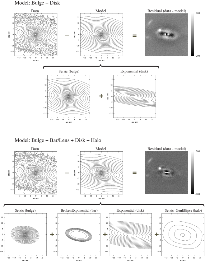
Figure 10: Comparison of different two-dimensional decompositions of NGC 307. For each model, we show in the first row the observed, logarithmically scaled data isophotes (VLT-FORS1 $R$-band, left), model isophotes (middle), and the residual image (data $-$ model, linear scaling from $-200$ to 200 counts/pixel; right). The individual components contributing to the model are show in the second row; components are identified by the name of the Imfit function used for each (see Erwin, 2015). Top pair of rows: best-fitting simple bulge + disc model. Bottom pair of rows: best-fitting bulge + bar/lens + disc + outer halo model. The range of isophote levels is the same for all contour plots, and both residual images use the same display range. North is up and east is to the left in all panels.

6.2.1 Generating Final “Bulge” and “Disc” Components for Dynamical Modeling

To generate “bulge-only” images for use in constructing the final bulge model, we constructed model images (using the makeimage tool in Imfit) consisting of the bar/lens, disc, and halo components of the best-fitting B+b+D+H model, suitably rescaled and PSF-convolved for the SINFONI, FORS1, and WFI images. These were then subtracted from the data images, and ellipses were fit to the resulting residual images. The final bulge profile consisted of ellipse-fit data from the residual SINFONI image for $a<1.1\arcsec$, FORS1 data for $a=1.1$–10″, and a Sérsic extrapolation of the inner data (using the bulge parameters in Table 1) for larger radii. The ellipticity and $\cos 4\theta$ values were taken from the residual SINFONI image ellipse fits for $a<1.1\arcsec$ and were set to 0.385 and 0, respectively, for larger radii.

The “disc-only” images used for constructing the final disc model (actually the disc + lens + stellar halo) were generated in an analogous fashion: PSF-convolved model-bulge images (using the inner Sérsic parameters from Table 1) were subtracted from the FORS1 and WFI images, and the resulting residual images were fit with both fixed and free ellipses. Since, as noted above, NGC 307 has a significant outer halo which is rounder than the disc, the final “disc” model actually incorporates a transition from the azimuthally averaged, constant-ellipticity profile to a profile with declining ellipticity at $a=28\arcsec$. The ellipticity and PA for the fixed-ellipse fits were 0.69 and 82°, based on free-ellipse fits to the residual FORS1 image; these values are almost identical to those of the exponential-disc component in the best-fitting B+b+D+H model (Table 1). The fixed-ellipse-fit FORS1 data were used for $a=6.4$ to 28″ in the final profile, with free-ellipse-fit surface-brightness and ellipticity used for $a\geq 28\arcsec$ (using WFI free-ellipse-fit data for $a>47\arcsec$). For $a<6.5\arcsec$, the FORS1 fixed-ellipse-fit surface brightness became extremely noisy and difficult to deproject; thus the surface-brightness data at smaller radii come from a fixed-ellipse fit to an unconvolved model image (built using the disc + bar/lens + halo components from Table 1). At these small radii the final luminosity density is dominated by the bulge component, so accuracy in the disc component is less important.

Figure 13 shows the surface-brightness profiles of the final bulge and disc components. The top panel of Figure 14 compares the surface-brightness profile of our final bulge component (red) with the equivalent (ellipse-fit-derived) surface-brightness profile of the Sérsic function (convolved with the SINFONI PSF) from our 2D decomposition. Although they are very similar, the final bulge component is brighter in the centre than the inward extrapolation of the Sérsic function. If we had simply used the Sérsic function itself as the bulge component for deprojection, we would underestimate the central stellar density and thus potentially overestimate the SMBH mass in our modeling. The bottom panel of the figure makes the same comparison for the disc component.

Ideally, one could treat the outer halo as a third stellar component, with its own $M/L$ ratio. However, since our kinematic data are limited to $r\la 30\arcsec$ along the major axis, well inside the region where the halo component begins to dominate over the disc (e.g., Figure 12), the precise details of the stellar halo do not significantly affect our dynamical modeling.

Table 1: NGC 307: 2D Photometric Decomposition

Component	Parameter	Value	$\sigma$	Units
Sersic	PA	82.41	0.18	deg
(bulge)	$\epsilon$	0.385	0.002
	$n$	2.548	0.041
	$\mu_{e}$	15.076	0.035	mag arcsec-2
	$r_{e}$	2.186	0.049	arcsec
BrokenExponential	PA	79.19	0.29	deg
(bar/lens)	$\epsilon$	0.552	0.005
	$\mu_{0}$	17.907	0.170	mag arcsec-2
	$h_{1}$	32.39	18.61	arcsec
	$h_{2}$	1.521	0.095	arcsec
	$R_{\rm brk}$	9.090	0.105	arcsec
	$\alpha$	10.0	—	arcsec-1
Exponential	PA	81.81	0.29	deg
(disc)	$\epsilon$	0.708	0.002
	$\mu_{0}$	16.509	0.017	mag arcsec-2
	$h$	11.04	0.08	arcsec
Sersic_GenEllipse	PA	76.80	0.90	deg
(halo)	$\epsilon$	0.349	0.003
	$c_{0}$	0.569	0.035
	$n$	0.972	0.016
	$\mu_{e}$	21.077	0.014	mag arcsec-2
	$r_{e}$	35.36	0.19	arcsec

Summary of the final 2D decomposition of the $R$-band VLT-FORS1 image of NGC 307 (using Imfit). Column 1: Imfit component names. Column 2: Parameter names. Column 3: Best-fit parameter value. Column 4: Nominal uncertainty on parameter value (from Levenberg-Marquardt minimization). Column 5: Units of the parameter. For all parameters of the Sersic_GenEllipse component except PA and $\mu_{e}$, the values come from fitting the WFI image and were held fixed during the fit to the FORS1 image. Surface brightnesses are in $K$-band.

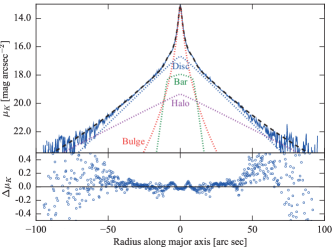
Figure 12: Upper panel: Major-axis cut through the VLT-FORS1 and WFI $R$-band images of NGC 307 (solid blue line, using FORS1 data for $|r|<22\arcsec$), along with major-axis cuts through best-fitting, PSF-convolved B+b+D+H model image (black dashed line) and through individual (PSF-convolved) components of the model image: Sérsic (bulge; red short-dashed line), broken-exponential (bar/lens; green short-dashed line), exponential (disc; blue short-dashed line), and outer Sérsic (halo; magenta short-dashed line). Lower panel: Residuals from fit ($\mu_{\rm data}-\mu_{\rm model}$) evaluated along the major-axis cut.

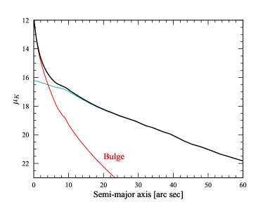
Figure 13: Final surface-brightness profiles used for constructing stellar luminosity-density components for NGC 307, showing $K$-band surface brightness versus semi-major axis for the “disc” (i.e., bar + disc + halo; cyan) and bulge (red) components, as well as their sum (thicker black line).

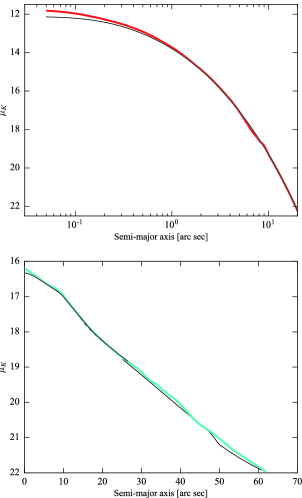
Figure 14: Top: Comparison of the final surface-brightness profile for the measured bulge component, used to construct the bulge luminosity-density component for our dynamical modeling (thick red line, same as in Figure 13), with the profile of the Sérsic component from our 2D decomposition (thin black line, convolved with the SINFONI PSF). Bottom: Comparison of the final disc component (thick cyan line, same as in Figure 13) with the profile of the exponential + broken-exponential + outer Sérsic components from our 2D decomposition (thin dashed black line = unconvolved model image, thin solid black line = convolved with VLT-FORS1 PSF); values at $a<28\arcsec$ are from fixed ellipse fits, while values at larger semi-major axis values are from free ellipse fits (see text).

6.3 Deprojection

To go from the surface-brightness profiles and the accompanying geometric information (ellipticity, $B_{4}$) to actual 3D luminosity density models requires deprojection under certain assumptions. We use an approach based on that of Magorrian (1999). Different realizations of 3D luminosity-density models are projected, assuming an inclination of 76°, and compared to the observed 2D surface-brightness model derived from the profiles. A simulated annealing algorithm is used to maximize a penalized log-likelihood function based on the difference between the model and the data in order to determine the best-fitting 3D model.

We performed separate deprojections for the bulge and disc components. Since the central regions of the disc component are negligible compared to the bulge component, we ignored the effects of PSF convolution (in fact, as explained in the previous section, the central part of our disc surface-brightness component was derived from an unconvolved model image). For the bulge component, on the other hand, PSF convolution is important, so we used our double-Gaussian model of the SINFONI PSF (Section 3.1) when projecting trial 3D bulge-component models for comparison with the data.

7 Dynamical Modeling

To determine the SMBH mass and stellar $M/L$ ratios for NGC 307, we use Schwarzschild orbit-superposition modeling (Schwarzschild, 1979) with the three-integral, axisymmetric code of Thomas et al. (2004), which is based in turn on the code of Gebhardt et al. (2003) (see also Siopis et al. 2009).

The basic outline of our Schwarzschild modeling process is as follows. First, we define general mass models consisting of a SMBH, one or more stellar components, and (optionally) a DM halo. Then, for each such model, we perform fits spanning a grid in the space of free parameters of the model, computing regularized $\chi^{2}$ values (see below) for each combination of parameters. Finally, we analyse the resulting $\chi^{2}$ landscape and the corresponding likelihoods to determine best-fit parameter values and corresponding confidence intervals.

The fitting process for a given general model is:

1. Construct a specific mass model and its potential from the general model, based on particular values for the free parameters (SMBH mass, stellar $M/L$ ratios, DM halo parameters).

2. Integrate test particles within this potential to build a library of orbits. For NGC 307, we used $2\times 14,300$ individual orbits, with the duplication achieved by reversing the angular momentum of individual orbits.

3. Assign weights $w_{i}$ to the individual orbits so that their weighted sum reproduces the input stellar mass model (this is treated as a boundary condition, so the match is exact to within machine tolerances) and reproduces the observed kinematics. The comparison with the kinematic data is done by simulating kinematic observations of the model using the same spatial and LOSVD bins as the data, convolved with PSFs based on the observations. A $\chi^{2}$ value is computed based on the comparison between the observed and model kinematics.

4. Repeat the process with new values of the free parameters.

The fit of a given orbit library to the kinematic data is computed by maximizing $\hat{S}=S-\alpha\chi^{2}$. This is a regularized version of a $\chi^{2}$ minimization, based on a maximum entropy approach, where $\alpha$ is the regularization parameter and $S$ is the Boltzmann entropy:

$$S\;=\;-\sum_{i}w_{i}\ln\left(\frac{w_{i}}{V_{i}}\right),$$ (3)

with $V_{i}$ the phase-space volume of orbit $i$, computed as in Thomas et al. (2004). The $\chi^{2}$ term is

$$\chi^{2}=\sum_{j=1}^{N_{L}}\sum_{k}^{N_{\rm vel}}\frac{(L_{jk,{\rm m}}-L_{jk,{\rm d}})^{2}}{\sigma_{jk}^{2}},$$ (4)

which is a sum over the $N_{L}$ spatial positions $j$ and the $N_{\rm vel}$ LOSVD bins $k$, with $L_{jk,{\rm m}}$ and $L_{jk,{\rm d}}$ the model and data values in each LOSVD bin and $\sigma_{jk}^{2}$ the corresponding Gaussian uncertainty for the data.

Since our modeling code assumes axisymmetry, we treat each quadrant of kinematic data as a separate dataset to which the model is fit. The result is four independent evaluations for each set of model parameters, which can in principle be used as quasi-independent estimates of model uncertainties, as well as a gauge of how well the underlying assumption of axisymmetry is justified (e.g., Nowak et al., 2010). Our final analysis is based on combining the results for all four quadrants, as described below.

We have four general models. Each features a central SMBH. Model A has single stellar component; Model A+DM adds a DM halo to this. Model B has two stellar components: one for the bulge sub-component and one for the disc; Model B+DM also includes a DM halo. These models are summarized in Table 2, and described in more detail in the following subsections.

The stellar density components are based on stellar luminosity density components $\nu$ (plus a $M/L$ ratio which converts luminosity to mass). The luminosity density components themselves are obtained by deprojecting the surface-brightness components (Section 6.3). For the single-stellar-component model, we simply add the bulge and disc luminosity-density models together and assign the result a single $M/L$ value.

To determine best-fit values and confidence intervals for parameters, we use a slightly modified version of the likelihood-based approach of McConnell et al. (2011) and Rusli et al. (2013). For each value of a given parameter (e.g., $M_{\rm BH}$), we compute the relative likelihood (from the $\chi^{2}$) for a given quadrant by marginalizing over the other parameters; the final relative likelihood is then the product of the likelihoods for the individual quarters. As an example, the marginalized likelihood value $\mathcal{L}_{n}(x)$ for a model with parameters $x$, $y$, and $z$, evaluated in quadrant $n$, would be:

$$\mathcal{L}_{n}(x)\;\propto\;\sum_{y_{\rm min}}^{y_{\rm max}}\sum_{z_{\rm min}}^{z_{\rm max}}e^{-\frac{1}{2}\chi_{n}^{2}(x,y,z)}\Delta z\,\Delta y,$$ (5)

and the final marginalized likelihood value would be

$$\mathcal{L}(x)\;=\;\prod_{n=1}^{4}\mathcal{L}_{n}(x).$$ (6)

To determine the best-fit values and confidence intervals, we use the cumulative of the marginalized likelihood:

$$C(x)\;=\;\frac{\int_{x_{\rm min}}^{x}\mathcal{L}(x^{\prime})\,\mathrm{d}x^{\prime}}{\int_{x_{\rm min}}^{x_{\rm max}}\mathcal{L}(x^{\prime})\,\mathrm{d}x^{\prime}}$$ (7)

with the best-fit value at the median, where $C(x)=\frac{1}{2}$, and the 68% (“1-$\sigma$”) confidence interval defined by the values of $x$ for which $C(x)=0.16$ and 0.84.

The best-fit parameter values and confidence intervals for each model are presented in Table 3, along with the total CPU time used for each model. The relative $\chi^{2}$ and marginalized likelihood plots for SMBH mass and stellar $M/L$ ratios for all four models are shown in Figure 15. The grey shaded areas show the (arbitrarily scaled) marginalized likelihood for the parameter in question, with the best-fit value and confidence intervals indicated by the solid and dashed vertical black lines. The lines show $\Delta\chi^{2}=\chi^{2}(x)-\chi^{2}_{0}$, where $\chi^{2}(x)$ is the minimum for all models with the same value of the parameter in question (marginalized over the other parameters) and $\chi^{2}_{0}$ is the minimum $\chi^{2}$ over all parameter values. The thin lines show the $\Delta\chi^{2}$ values for the individual-quadrant fits; the thick lines are the result of summing the individual-quadrant $\chi^{2}$ values.

Table 2: NGC 307: Summary of Dynamical Models

Model Name	Stellar Component(s)	DM halo	$N_{\rm free}$
(1)	(2)	(3)	(4)
A	Single $\Upsilon_{\rm tot}$	No	2
A+DM	Single $\Upsilon_{\rm tot}$	Yes	4
B	$\Upsilon_{\rm bulge}$, $\Upsilon_{\rm disc}$	No	3
B+DM	$\Upsilon_{\rm bulge}$, $\Upsilon_{\rm disc}$	Yes	5

Summaries of the different dynamical models fit to the kinematic data of NGC 307. (1) Name of model. (2) Stellar component(s) = whether a single stellar component (one $M/L$ ratio) or separate bulge and disc components with independent $M/L$ ratios were used. (3) DM halo = whether a dark-matter halo was used in the model. (4) The number of free parameters in the model.

7.1 Model A: SMBH + Single Stellar Component

Model A is is the traditional model used for most published dynamical SMBH mass measurements. It consists of a SMBH and a single stellar-density component:

$$\rho\;=\;M_{\rm BH}\,\delta(r)\>+\>\Upsilon_{\rm tot}\,\nu_{\rm tot}.$$ (8)

For NGC 307, the single luminosity-density component $\nu_{\rm tot}$ is the sum of the bulge and disc luminosity-density components $\nu_{b}$ and $\nu_{d}$, which are the deprojections (Section 6.3) of the bulge and disc surface-brightness profiles derived in Section 6.2.1.

The relative $\chi^{2}$ and marginalized likelihood plots for this model are shown in the upper left part of Figure 15. The best-fit SMBH mass ($7\pm 1\times 10^{7}M_{\sun}$) is rather low – about a factor of four smaller than what the $M_{\rm BH}$–$\sigma$ would predict (see Section 8.1) – though by itself not obviously implausible. The stellar $M/L$ is apparently quite well-defined.

7.2 Model A+DM: SMBH + Single Stellar Component + DM Halo

Model A+DM is Model A with the addition of a dark-matter halo, so that the mass model is

$$\rho\;=\;M_{\rm BH}\,\delta(r)\>+\>\Upsilon_{\rm tot}\,\nu_{\rm tot}\>+\>\rho_{\rm DM}.$$ (9)

The DM halo is a standard spherical cored logarithmic model (e.g., Binney & Tremaine, 1987), with a density profile given by

$$\rho_{\rm DM}(r)\;=\;\frac{V_{h}^{2}}{4\pi G}\frac{3r_{h}^{2}+r^{2}}{(r_{h}^{2}+r^{2})^{2}},$$ (10)

where $r_{h}$ is the core radius (inside of which the density slope is constant) and $V_{h}$ is the asymptotic circular velocity. Previous studies modeling early-type galaxies with DM haloes have found that similar results are obtained for both cored logarithmic and NFW DM halo models (Thomas et al., 2005, 2007). Schwarzschild modeling of SMBH masses including DM haloes have also found that the results do not depend strongly on the specific DM halo model used (Gebhardt & Thomas, 2009; McConnell et al., 2011).

The lower left part of Figure 15 shows relative $\chi^{2}$ and marginalized likelihood plots for Model A+DM. The SMBH mass ($2.0\pm 0.3\times 10^{8}M_{\sun}$) is about three times larger than the Model A value; the stellar $M/L$ ratio is about 15% smaller ($\Upsilon_{K,{\rm tot}}=1.1\pm 0.1$).

Model A+DM required almost 30 times the computational effort of Model A.

7.3 Model B: SMBH + Bulge + Disc

Model B is similar to Model A except that there are two stellar-density components in the mass model, each with its own $M/L$ ratio, so the mass model is

$$\rho\;=\;M_{\rm BH}\,\delta(r)\>+\>\Upsilon_{\rm bulge}\,\nu_{\rm b}\>+\>\Upsilon_{\rm disc}\,\nu_{\rm d},$$ (11)

where $\nu_{\rm b}$ and $\nu_{\rm d}$ are the bulge and disc luminosity-density models, respectively. These two components are deprojections (Section 6.3) of the bulge and disc surface-brightness models derived in Section 6.2.1.

Relative $\chi^{2}$ and marginalized likelihood values for this model are shown in the upper right part of Figure 15. The disc-component $M/L$ value ($\Upsilon_{\rm disc}$) is implausibly high ($1.9\pm 0.1$); however, the bulge $M/L$ value ($1.1\pm 0.1$) is lower than the global $M/L$ of Model A, and is in fact identical to the global $M/L$ value of Model A+DM. The SMBH mass ($3.0\pm 0.5\times 10^{8}M_{\sun}$) is about 50% larger than that from Model A+DM, but still consistent with the latter at the $\sim 2-\sigma$ level; it is over four times larger than the Model A value.

Model B required about six times the computational effort as Model A, but only one-fifth that of Model A+DM.

Table 3: NGC 307: Best-Fit Results from Dynamical Modeling

Model Name	$M_{\rm BH}$	$\Upsilon_{\rm tot}$	$\Upsilon_{\rm bulge}$	$\Upsilon_{\rm disc}$	$r_{h}$	$V_{h}$	$t_{\rm comp}$
	($10^{8}M_{\sun}$)				(kpc)	(km s-1)	(CPU h)
(1)	(2)	(3)	(4)	(5)	(6)	(7)	(8)
A	$0.70\pm 0.1$	$1.3\pm 0.1$	—	—	—	—	12001
A+DM	$2.0\pm 0.5$	$1.1\pm 0.1$	—	—	$>4.5$	$200\pm 20$	33000
B	$3.0\pm 0.5$	—	$1.1\pm 0.1$	$1.9\pm 0.1$	—	—	7400
B+DM	$2.2\pm 0.6$	—	$1.1\pm 0.1$	$1.0\pm 0.1$	$>5.6$	$260\pm 30$	200000

Final results of dynamical modeling for NGC 307. (1) Model Name – see Table 2. (2) SMBH mass. (3) $K$-band stellar $M/L$ ratio for combined stellar component. (4) $K$-band stellar $M/L$ ratio for bulge component. (5) $K$-band stellar $M/L$ ratio for disc component. (6) DM halo radius. (7) DM halo circular velocity. (8) Total computation time in CPU hours. Notes: 1. Some additional time was spend exploring the low-$M_{\rm BH}$ part of parameter space for this model, since the standard parameter-grid exploration yielded only an upper limit on $M_{\rm BH}$.

Table 4: NGC 307: Comparison of Models

Model	Q1	Q2	Q3	Q4
AIC values
A	728.6	574.9	1075.2	964.1
A+DM	692.7	508.7	1050.9	918.3
B	694.9	518.4	1051.4	917.5
B+DM	694.3	504.6	1050.4	916.0
BIC values
A	738.7	585.0	1085.5	974.5
A+DM	717.9	534.0	1076.6	941.8
B	710.1	533.6	1066.9	933.0
B+DM	719.6	529.9	1076.1	941.8

Comparison of different models fit to the NGC 307 data. Since each model was fit to the kinematic data in each quadrant separately, we list the corresponding Akaike Information Criterion (AIC) and Bayesian Information Criterion (BIC) values for each quadrant (Q1, Q2, Q3, Q4) separately. (See Figure 4 for how the quadrants were specified.) Lower values of AIC or BIC indicate better matches between model and data for a given quadrant (accounting for differences in the number of free parameters).

7.4 Model B+DM: SMBH + Bulge + Disc + DM Halo

Model B+DM is the most complex model we consider. It is the same as Model B except that there is also a DM halo, so the that the mass model is

$$\rho\;=\;M_{\rm BH}\,\delta(r)\>+\>\Upsilon_{\rm bulge}\nu_{\rm b}\>+\>\Upsilon_{\rm disc}\nu_{\rm d}\>+\>\rho_{\rm DM}.$$ (12)

The DM halo is the same spherical cored logarithmic model as we use in Model A+DM. The combined model thus has a total of five free parameters: $M_{\rm BH}$, $\Upsilon_{\rm bulge}$, $\Upsilon_{\rm disc}$, $r_{h}$, and $V_{h}$.

The lower right part of Figure 15 shows relative $\chi^{2}$ and marginalized likelihood values for the SMBH mass and the $M/L$ ratios for the bulge and disc components. The best-fit $M_{\rm BH}$ value ($2.2\pm 0.6\times 10^{8}M_{\sun}$) is in between the best-fit values from Model A+DM and Model B, and is more than three times larger than the best-fit value from Model A. The bulge $M/L$ value is identical to the value in Model B (and the global $M/L$ ratio of Model A+DM). The disc $M/L$ value ($1.0\pm 0.1$) is only about 60% of the value in Model B, and is thus now lower than the bulge $M/L$ ratio, in qualitative agreement with our spectroscopic analysis (Section 5).

Since we consider this the best model for NGC 307 (see discussion below), we show details of the fits to the kinematic data in Figures 16. This compares the predicted stellar kinematics from the best-fit model with the kinematic data from each of the four quadrants; note that for simplicity we show Gauss-Hermite moments – $V$, $\sigma$, $h_{3}$, and $h_{4}$ – derived from the full LOSVDs.

With a total of five free parameters, Model B+DM required 200,000 CPU hours of computational time – six times that of the other DM-halo model (Model A+DM) and almost 30 times that of Model B.

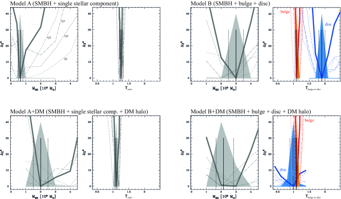
Figure 15: Relative $\chi^{2}$ and marginalized likelihood plots for the dynamical modeling of NGC 307, comparing all four general models. For each model, we show $\Delta\chi^{2}=\chi^{2}-\chi^{2}_{\rm min}$ values with gray, red, or blue lines, with thin lines showing values for modeling of individual quadrants of kinematic data (Q1 = dotted, Q2 = short-dashed, Q3 = long-dashed, Q4 = dot-dashed) and thick lines showing the sum over all four quadrants. Likelihood values (combining results for all four quadrants) are indicated by the gray, blue, or orange shading; the likelihoods are scaled to an arbitrary maximum value of 40 in each panel. Vertical solid lines mark best-fit values for each parameter and vertical dashed lines indicate 68% confidence intervals. For each model, the left-hand panels show black hole mass, while the right-hand panels show stellar $M/L$ values for the single-stellar components of Models A and A+DM, or for the bulge [red] and disc [blue] components of Models B and B+DM. Upper left pair of panels: Model A (SMBH + single stellar component). Lower left pair of panels: Model A+DM (same as Model A, but with DM halo added). Upper right pair of panels: Model B (SMBH + separate bulge and disc stellar components). Lower right pair of panels: Model B+DM (same as Model B, but with DM halo added).

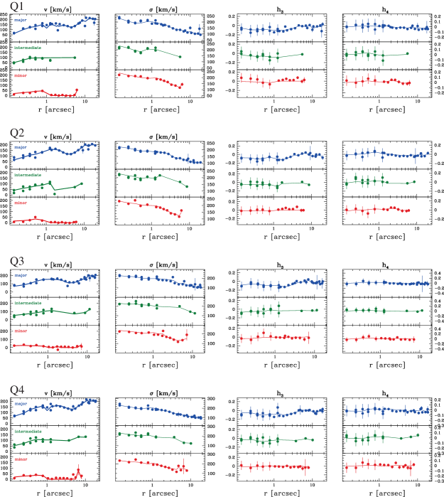
Figure 16: Comparison of Gauss-Hermite kinematic data (points) and best-fitting model predictions from Model B+DM (lines) for kinematic data from the four quadrants (Quadrants 1–4 are presented one per row, from top to bottom). For each quadrant, we plot $V$, $\sigma$, $h_{3}$, and $h_{4}$ extracted along the major (upper sub-panels, blue), intermediate (middle sub-panels, green), and minor (lower sub-panels, red) axes, along with corresponding values from the best-fit model for that quadrant. Note that models were fit to the full LOSVDs from the 2D data in each quadrant, not to the Gauss-Hermite moments plotted in the figure.

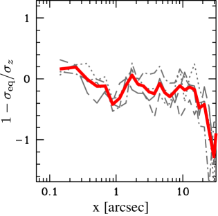
Figure 17: Plots of orbital equatorial anisotropy for the orbits in our preferred best-fit model (Model B+DM). We show $1-\sigma_{eq}^{2}/\sigma_{z}^{2}$, where $\sigma_{eq}$ is the equatorial dispersion ($\sigma_{eq}^{2}=\sigma_{r}^{2}+\sigma_{\phi}^{2}$) and $\sigma_{z}$ is the vertical dispersion. The thin black lines represent results from models to the individual quadrants; the thick red line is the mean. The overall trend is for isotropic dispersion out to a radius of $\sim 10\arcsec$, with increasingly strong equatorial anisotropy (as expected for a rotationally dominated disc) outside.

7.5 Comparison and Summary of Modeling

The effect of not including a DM halo in the single-stellar-component case (Model A) is easily understood, because it is similar to the effects seen for elliptical galaxies (always modeled as single-stellar-component systems). Without a DM halo, the stellar component needs a higher $M/L$ ratio ($\Upsilon_{\rm tot}=1.3$) in order to match the observed kinematics at large radii, where the (real) DM halo starts to become significant compared to the stars. Since the stellar $M/L$ ratio is the same at all radii, this effect also increases the stellar mass in the inner regions of the galaxy, and so a lower SMBH mass is needed to in order to match the observed kinematics there.

When a DM halo is added to Model A (creating Model A+DM), the effect is fairly dramatic: although the stellar $M/L$ ratio decreases only moderately (from 1.3 to 1.1), the SMBH is almost three times larger ($M_{\rm BH}=2.0\pm 0.5\times 10^{8}M_{\sun}$). As is true for elliptical galaxies modeled with DM haloes, the halo is able to replace the role of the stellar component in accounting for the outer kinematics. Consequently, the stellar component can acquire a lower value, and the SMBH mass can correspondingly increase.

For Model B (the two-stellar-component model without DM halo), the disc component is affected in a fashion similar to (but even stronger than) that of the single stellar component in Model A: in order to explain the observed kinematics at large radii, the disc $M/L$ ratio is biased high ($\Upsilon_{\rm disc}=1.9$) to compensate for the absence of a DM halo. However, the presence of a separate bulge stellar component – which dominates the stellar mass budget at small radii – breaks the direct connection between outer stellar $M/L$ ratio and SMBH mass that bedevils Model A. Instead, the bulge $M/L$ ratio and the SMBH mass can vary as needed to better match the observed central kinematics. The result is a lower $M/L$ ratio for the bulge component and a higher mass for the SMBH. The bulge $M/L$ value ($\Upsilon_{\rm bulge}=1.1\pm 0.1$) is identical to the global stellar $M/L$ value in Model A+DM; the SMBH mass is only 50% higher. The only obvious problem with Model B is the unrealistically high $M/L$ ratio for the disc component – almost twice the bulge $M/L$ ratio. This is directly contradicted by the stellar-population analysis in Section 5, which indicated that the disc $M/L$ ratio should be lower than the bulge $M/L$ ratio.

Adding a DM halo to Model B (Model B+DM) primarily affects the disc $M/L$ ratio: instead of there needing to be excess stellar mass at large radii in order to explain the observed kinematics, mass can be shifted into the DM halo component. The result is a much lower – and much more plausible – $M/L$ ratio for the disc component of $\Upsilon_{\rm disc}=1.0$. Because the outer stellar component remains decoupled from the inner component, the effect on the bulge $M/L$ ratio and thus the SMBH mass is relatively mild. In fact, the bulge $M/L$ ratio is unchanged from the Model B value, and the SMBH mass is in between the values for Model A+DM and Model B.

Because our kinematic data do not extend much beyond the baryon-dominated inner regions of the galaxy, they cannot provide strong constraints on the DM halo. In practice, fitting the two models with a DM halo component (A+DM and B+DM) yields only lower limits on the halo radius and somewhat discordant asymptotic velocities ($200\pm 20$ km s^-1 for A+DM, $260\pm 20$ km s^-1 for B+DM).

Do the models with extra components provide significantly better fits to the data in a purely statistical sense? Since we are comparing multiple models which are not simply nested (e.g., while Model A is nested within Model A+DM, Models B and B+DM are not), direct comparisons of $\chi^{2}$ values is not valid. Instead, we look at more general comparisons using information-theoretic statistics, which can be used to compare non-nested models that are fit to the same data. Table 4 compares the best fits of the different models using the Akaike Information Criterion (AIC; see Section 6.2) and also the Bayesian Information Criterion (Schwarz, 1978). The AIC (actually the “corrected” AIC_c value) and BIC values are calculated using the $\chi^{2}$ term from Eqn. 4. As noted in Section 6.2, lower values of AIC (or BIC) indicate better fits; differences of $<2$ are insignificant, while differences of $>6$ are considered strong evidence that the model with the lower AIC or BIC is superior.

In this context, Model A is clearly the worst model: its AIC values are $\sim 9$–55 higher than those of the other models, and its BIC values are 24–70 higher. The other models are practically indistinguishable from each other in terms of AIC and BIC values. For example, only for the Q2 value is Model B+DM clearly superior to Model B. The BIC values actually favor Model B over Model B+DM ($\Delta$BIC $\approx 9$) for all datasets except Q2.

What this shows is that our kinematic data are insufficient to clearly discriminate between Models A+DM, B, and B+DM. The data, for example, do not allow us to distinguish between the case of a massive disc with no DM halo (Model B) and the case of a low-mass disc with a DM halo (Model B+DM).

7.6 Variations: Testing the Sensitivity of Fits to Bulge/Disc Decompositions

The method we use for generating the luminosity-density models involves a 2D bulge-disc decomposition (with multiple sub-components for the “disc”). Uncertainties in this process translate into uncertainties in the amount of light assigned to different components. Since for Models B and B+DM we assign potentially different $M/L$ ratios to the bulge and disc components, the decomposition uncertainties could, in principle, affect our derived $M/L$ ratios and SMBH masses.

To test how much variations in the bulge/disc decomposition might actually affect the derived model parameters, we ran additional fits of Model B using divergent versions of our bulge/disc decompositions corresponding to 1-$\sigma$ deviations from the best fit. This is described in more detail in Appendix A. The results can be summarized as effectively no discernable changes in the black hole mass or stellar $M/L$ ratios for fits using $\pm 1$-$\sigma$ variations on the best-fit decomposition, so we conclude that our results are not significantly affected by uncertainties in the decomposition.

7.7 Which Model Is Best? Accuracy Versus Efficiency and Strategies for Modeling

We are left with three models – A+DM, B, and B+DM – which are approximately equally good at fitting the kinematic data. How can we choose among them? From a general astrophysical perspective, Model B+DM should be the most correct (or least wrong) model, since it allows for both the possibility of different bulge and disc stellar $M/L$ ratios (something we expect from both our general understanding of disc galaxy evolution and from the spectroscopic evidence for NGC 307 itself) and the existence of a separate DM halo (something we expect for all galaxies). The fact that the derived bulge and disc $M/L$ ratios for Model B+DM qualitatively agree with the spectroscopic results (slightly higher in the bulge-dominated region, lower in the disc outside; Section 5) is further reason to prefer it over the other models, although given the uncertainties in $M/L$ ratios, its superiority relative to the Model A+DM is not statistically significant. Although Model B allows for different $M/L$ ratios in the bulge and disc regions, its agreement with the spectroscopic analysis is actually worse, because it has a disc $M/L$ ratio that is higher than the bulge value. Moreover, its disc $M/L$ value ($\Upsilon_{\rm disc}=1.9$) is too high to be physically plausible.

While the best model for NGC 307 is thus probably Model B+DM, it does have one practical drawback: the extensive computational time required to evaluate it (200,000 CPU hours in our case). The difficulty posed by computational time for Schwarzschild modeling is illustrated by the fact that recent studies which used the equivalent of our Model A+DM – that is, including two DM halo parameters as part of the fit, for a total of four free parameters – have been devoted to one or at most two galaxies only (e.g., Gebhardt & Thomas, 2009; Shen & Gebhardt, 2010; Jardel et al., 2011; van den Bosch et al., 2012; Walsh et al., 2015; Yıldırım et al., 2015; Thomas et al., 2016; Walsh et al., 2016). Studies which included DM haloes for more than two galaxies have avoided the expense of full parameter-space searches by using fixed DM haloes in their models. Schulze & Gebhardt (2011) specified fixed halo parameters based on galaxy luminosity, while Rusli et al. (2013) first fit three-parameter stars + DM halo models (excluding the high-spatial-resolution data which probed the SMBH region) to derive halo parameters as a function of $\Upsilon_{\rm tot}$, and then fit SMBH + stars + DM halo models – with only $M_{\rm BH}$ and $\Upsilon_{\rm tot}$ as free parameters – to their full kinematic data. Schwarzschild modeling with five free parameters, as in our Model B+DM, has not previously been attempted, and is probably not (yet) a practical approach for more than one or two galaxies at a time.

If we are interested in measuring reasonably accurate SMBH masses, and potentially bulge $M/L$ ratios as well, for several galaxies at a time, then Models A+DM and B seem equally apropos: they yield SMBH masses close to the Model B+DM value and the same stellar $M/L$ ratio for the bulge region as in Model B+DM. Model A+DM has a somewhat more accurate SMBH mass, while Model B is clearly the most efficient way to measure these quantities, since it has only three free parameters and requires only $\sim 20$% as much computational time as Model A+DM.

8 Discussion

8.1 The SMBH in NGC 307

Our preferred model (Model B+DM) gives a SMBH mass of $M_{\rm BH}=2.2\pm 0.6\times 10^{8}M_{\sun}$ for NGC 307. Given the previously published central velocity dispersion of 205 km s^-1 (Saglia et al., 2016) and our adopted distance of 52.8 Mpc, the diameter of the black hole’s sphere of influence would be $\approx 0.18\arcsec$. Our SINFONI observations had a mean FWHM of $0.18\arcsec$, which means that our data (just) resolve the SMBH’s sphere of influence.

From the $M_{\rm BH}$–$\sigma$ relation of Saglia et al. (2016) we would derive an estimated SMBH mass of $2.67\times 10^{8}M_{\sun}$. Using the Sérsic model from our 2D decomposition in Section 6.2, the bulge of NGC 307 has $M_{K}=-22.65$; with the bulge $M/L$ from Model B+DM, this gives $M_{\rm bulge}=2.97\times 10^{10}M_{\sun}$, so the SMBH is 0.74% of the bulge mass. The predicted SMBH mass from the CorePowerEClassPC $M_{\rm BH}$–$M_{\rm bulge}$ relation in Saglia et al. (2016) would be $1.40\times 10^{8}M_{\sun}$. The SMBH in NGC 307 is thus within $\sim 30$–40% of what the $M_{\rm BH}$–$\sigma$ and $M_{\rm BH}$–$M_{\rm bulge}$ relations would predict, and is therefore quite unexceptional.

8.2 Implications for SMBH Measurements in Disc Galaxies

Our analysis of NGC 307 suggests that attempts to measure SMBH masses in disc galaxies via stellar-dynamical modeling can suffer from the same limitations that have been found for elliptical galaxies. Specifically, modeling a disc galaxy with just a single stellar component (with a uniform $M/L$ ratio) and a SMBH can lead to underestimated SMBH masses and overestimated stellar $M/L$ ratios. This can be alleviated by subdividing the stellar model into bulge and disc components (increasing the number of free parameters to three), or by adding a DM halo to the single-stellar-component model (increasing the number of free parameters to four). The best approach is clearly to model multiple stellar components and a DM halo, but this is computationally very expensive, since it involves five free parameters rather than three or four.

Schwarzschild modeling of disc galaxies using a single stellar component and no DM halo does not always lead to biased SMBH mass measurements, as the case of NGC 4258 shows. Siopis et al. (2009) obtained a SMBH mass measurement for that galaxy which differed by only $\sim 15$% from the very high quality maser measurement. Rusli et al. (2013) showed that biases to SMBH measurements without DM haloes in elliptical galaxies could be avoided if the inner kinematic data used in the modeling had sufficiently high spatial resolution – ideally several times better than the SMBH’s sphere of influence. Since the HST STIS kinematic observations used for the Siopis et al. analysis of NGC 4258 (FWHM $\approx 0.1\arcsec$) significantly over-resolved the SMBH sphere of influence ($d\approx 0.7\arcsec$, assuming $\sigma=115$ km s^-1, $D=7.27$ Mpc, and $M_{\rm BH}=3.8\times 10^{7}M_{\sun}$ from the compilation in Saglia et al. 2016), Schwarzschild modeling of the SMBH mass would understandably be insensitive to the lack of a DM halo.

Based on our findings, and by analogy with the results for elliptical galaxies, it seems plausible that disc galaxies where the SMBH sphere of influence is only just resolved – or is under-resolved – would be the likeliest candidates to have biased SMBH measurements when modeled with only one $M/L$ ratio and no DM halo. From the recent compilation of Saglia et al. (2016), there are eighteen disc galaxies with SMBH masses from Schwarzschild modeling. Four of these have been modeled with a single stellar component and a DM halo (Schulze & Gebhardt, 2011; Walsh et al., 2016), and another four were modeled with two stellar components (Davies et al., 2006; Nowak et al., 2010; Rusli et al., 2011). Of the remainder, we can identify two for which the FWHM of the kinematic observations is $\ga$ the diameter of the sphere of influence: NGC 1023 (Bower et al. 2001; FHWM = 0.2″, $d_{\rm SoI}=0.16\arcsec$) and NGC 2549 (Krajnović et al. 2009; FWHM = 0.17″, $d_{\rm SoI}=0.10\arcsec$). We suggest that those two galaxies in particular could benefit from remodeling with multiple stellar components or with DM haloes (or both).

8.3 Stellar Orbital Structure

Schwarzschild modeling produces a distribution of weights for the different pre-calculated orbits in the model potential. From these, it is possible to learn something about the stellar orbital structure in the best-fitting model. As we have done in past studies (e.g., Thomas et al., 2014; Erwin et al., 2015), we examine the radial trend in orbital anisotropy. Specifically, we adopt the approach of Erwin et al. and calculate an anisotropy parameter using the ratio of planar/equatorial velocity dispersion $\sigma_{eq}$ to the vertical velocity dispersion $\sigma_{z}$ (assuming cylindrical coordinates $R,\varphi,z$), where the mean dispersion in the equatorial plane is defined by

$$\sigma_{eq}^{2}=(\sigma_{R}^{2}+\sigma_{\varphi}^{2})/2\,.$$ (13)

We compute the averages at each radius from orbits in angular bins that range from $\theta=-23\degr$ to $\theta=+23\degr$ with respect to the equatorial plane. The anisotropy $\beta_{\rm eq}=1-\sigma_{eq}^{2}/\sigma_{z}^{2}$ is $\sim 0$ for isotropic velocity dispersion and $<0$ for planar-biased anistropy; values of $\sim-1$ are typical for the Galactic disc in the Solar neighborhood (e.g., Bond et al., 2010).

Figure 17 shows that isotropy ($\beta_{\rm eq}\sim 0$) is the rule for $r\la 12\arcsec$. For $r\la 5\arcsec$, this is consistent with the evidence from the photometric decomposition and the stellar-population analysis for a classical bulge. The region $r\sim 5$–12″ is outside the bulge, and so at first glance it is puzzling that the velocity dispersion remains roughly isotropic. However, $r\sim 12$ is roughly where our exponential-disc component begins to dominate the light (see Figure 12). This suggests that the near-isotropy between $\sim 5$ and 12″ may be related to the weak bar or lens, which contributes to the light in that radial range. We note that although lenses are in general poorly studied, some previous stellar-kinematic observations and models of barred galaxies have suggested that lenses are kinematically hot, possibly dominated by chaotic orbits or a large fraction of retrograde orbits (e.g., Kormendy, 1983, 1984; Pfenniger, 1984; Teuben & Sanders, 1985; Harsoula & Kalapotharakos, 2009). Thus, is it perhaps not surprising that the lens region in NGC 307 fails to show the rotation-dominated anisotropy of a classical disc.

9 Summary

We have presented 2D photometric decompositions, stellar kinematics from adaptive-optics IFU and large-scale IFU and long-slit spectroscopy, and dynamical modeling of the S0 galaxy NGC 307 with the aim of determining the mass of its central SMBH. We have paid particular attention to the effects of modeling the stellar component as a single entity with one $M/L$ ratio versus modeling it as two sub-components (bulge and disc) with independent $M/L$ ratios, and the effects of including a separate DM halo in the modeling.

Our best estimate, from the model with a SMBH, separate bulge and disc components, and a DM halo (Model B+DM), is a black hole mass of $2.2\pm 0.6\times 10^{8}M_{\sun}$, $K$-band bulge and disc $M/L=1.1\pm 0.1\,M_{\odot}/L_{\odot}$ and $1.0\pm 0.1\,M_{\odot}/L_{\odot}$, respectively, and a DM halo (spherical cored logarithmic model) with core radius $r_{c}>5.6$ kpc and circular velocity $V_{h}=260\pm 30$ km s^-1. The SMBH mass is within $\sim$ 40% of the predicted value from the $M_{\rm BH}$–$\sigma$ relation (assuming $\sigma_{0}=205$ km s^-1) and is $\approx 0.74$% of the bulge stellar mass, making NGC 307 entirely consistent with standard SMBH-bulge relations. The $M/L$ ratios are qualitatively consistent with single-stellar-population modeling of our long-slit spectroscopy, which implies a higher $M/L$ in the bulge region.

Modeling the stellar kinematics with both stellar components but without the DM halo (Model B) produces identical results for the bulge $M/L$ ratio ($1.1\pm 0.1\,M_{\odot}/L_{\odot}$) and a slightly higher SMBH mass ($3.0\pm 0.5\times 10^{8}M_{\sun}$). The disc $M/L$ ratio is significantly higher ($1.9\pm 0.1\,M_{\odot}/L_{\odot}$), due to the fact that the disc component has to be more massive to account for the effects of the (missing) halo. This approach requires only $\sim 4$% of the computational time as Model B+DM.

Modeling with a single stellar $M/L$ for both bulge and disc plus a DM halo (Model A+DM) yields a SMBH mass almost identical to that of Model B+DM ($2.0\pm 0.5\times 10^{8}M_{\sun}$) and a combined stellar $M/L=1.1\pm 0.1\,M_{\odot}/L_{\odot}$; the DM halo then has core radius $r_{c}>4.5$ kpc and circular velocity $V_{h}=200\pm 20$ km s^-1. The computational time required for this model is $\sim 20$% of the time required for model B+DM, but about 4.5 times that for Model B.

Finally, the simplest model, with a single stellar $M/L$ ratio and no DM halo, gives a much lower value for the SMBH mass ($7.0\pm 0.1\times 10^{7}M_{\sun}$) and a higher stellar $M/L$ ratio ($1.3\pm 0.1\,M_{\odot}/L_{\odot}$), because the necessity of accounting for the DM halo drives the stellar $M/L$ ratio to high values, increasing the stellar mass everywhere and reducing the amount of mass that can be assigned to the SMBH. This model is also clearly worse than the others in terms of how poorly it fits the kinematic data.

This suggests that dynamical modeling of disc galaxies can yield reasonably accurate measurements of SMBH masses and bulge $M/L$ ratios without needing the additional computational time of including a DM halo – if a separate disc component with its own $M/L$ ratio is included, though the disc $M/L$ ratio will then almost certainly be overestimated. Models that treat the entire galaxy as having a single stellar $M/L$ ratio (without a DM halo) can potentially underestimate the SMBH mass by significant amounts, especially if the kinematic data used do not overresolve the SMBH sphere of influence, as has been previously found for elliptical galaxies. We suggest that previous SMBH measurements for the S0 galaxies NGC 1023 and NGC 2549 should be revisited, since they were modeled using single stellar components and no DM haloes, using kinematic data which probably does not fully resolve their SMBH spheres of influence.

Our morphological and spectroscopic analysis of NGC 307, including 2D decompositions, suggests that the galaxy has four distinct stellar components: a compact central bulge with a metal-rich stellar population ($\approx 33$% of the light), a weak bar or lens ($\approx 6$%), an exponential disc ($\approx 36$%), and a rounder, luminous stellar halo with slightly boxy isophotes ($\approx 25$%) which is misaligned by about 5° with respect to the disc and bulge. (In our two-stellar-component dynamical modeling, we treated the disc + bar/lens + stellar halo as one component.) Using our best-fit $K$-band $M/L$ values, the estimated stellar masses for these components are $3.6\times 10^{10}M_{\sun}$ (bulge), $4.3\times 10^{9}M_{\sun}$ (bar/lens), $2.7\times 10^{10}M_{\sun}$ (disc), and $1.9\times 10^{10}M_{\sun}$ (stellar halo), with a total stellar mass of $8.6\times 10^{10}M_{\sun}$. The stellar halo is best understood as a separate component rather than being simply the outer part of the bulge; this is consistent with recent 2D decomposition analyses of the Sombrero Galaxy, which indicate a bulge + stellar halo + disc model is a better match to the galaxy than a single bulge component plus the disc (Gadotti & Sánchez-Janssen, 2012).

Appendix A Effects of Variation in Bulge/Disk Decomposition on Dynamical Modeling

Our preferred dynamical models (Models B and B+DM) have separate bulge and “disc” (i.e., disc + bar/lens + stellar halo) stellar components, each with its own $M/L$ ratio. There is the possibility that uncertainties in the bulge/disc decomposition (Section 6.2) – e.g., how much stellar light is assigned to the bulge component – might lead to uncertainties in the two stellar $M/L$ ratios, and thus potentially also to uncertainties in the SMBH mass. To investigate the possible effects of variations in the bulge-disk decomposition, we focused on the fits to the VLT-FORS1 image (Section 6.2). Using the bootstrapping facility in Imfit (see Section 5 of Erwin 2015), we generated 1000 resampled versions of the FORS1 image and fit each with the same B+b+D+H model as we used for the main decomposition (Table 1). We then computed the $B/T$ values for each best-fitting model. The standard deviation of the 1000 $B/T$ values was $\sigma_{B/T}=0.0046$ or $\sim 1.4$% of the original best-fit model’s $B/T$ of 0.3265.

We selected two of the bootstrap-resampled fits, with $B/T$ values equal to the best-fit value $\pm\sigma_{B/T}$. We then generated bulge and disc model surface-brightness profiles and deprojected these to form bulge and disc luminosity-density components, as in Section 6.3. Finally, we ran our dynamical modeling process using these new stellar components. For the underlying general dynamical model we used Model B, which has SMBH, bulge, and disc components. (We chose this general model because it contains separate bulge and disc $M/L$ ratios but requires considerably less time to run than Model B+DM.)

The results of the dynamical fits to these two decompositions are shown in Figure 18. The SMBH mass is, within in our admittedly somewhat coarse sampling, identical to our standard best-fit results ($M_{\rm BH}=3.0\pm 0.5\,M_{\sun}$) for Model B (see Table 3). The bulge and disc $M/L$ ratios are also identical ($\Upsilon_{\rm bulge}=1.1$, $\Upsilon_{\rm disc}=1.9$). We conclude that the nominal uncertainties of our bulge-disc decomposition have minimal effect on the results of our dynamical modeling, and in particular have negligible effect on the SMBH mass determination.

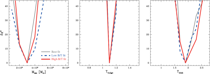
Figure 18: Marginalized likelihood plots for Model B (disc + bulge + SMBH, no DM halo) using alternate bulge/disc decompositions, for the SMBH mass (left), bulge $M/L$ (middle), and disc $M/L$ (right); see Appendix A for details. The dashed blue and solid red curves are for the low- and high-$B/T$ decompositions, respectively; the thinner dark grey curves are for the fit using the best decomposition (same as in the upper-right panel of Figure 15).

Appendix B Long-Slit Stellar Kinematics for NGC 307

The stellar kinematics (both major- and minor-axis) from our long-slit spectra of NGC 307 are presented in Table 5.

Table 5: VLT-FORS1 Stellar Kinematics

PA	R	V	err	$\sigma$	err	$h_{3}$	err	$h_{4}$	err
(°)	(″)	(km s-1)	(km s-1)	(km s-1)	(km s-1)
(1)	(2)	(3)	(4)	(5)	(6)	(7)	(8)	(9)	(10)
78.1	$-$24.71	215.43	7.80	88.71	10.91	$-$0.066	0.086	$-$0.102	0.052
78.1	$-$22.68	196.03	4.40	96.95	5.86	$-$0.054	0.053	$-$0.075	0.040
78.1	$-$20.43	204.41	5.67	106.02	6.29	$-$0.050	0.049	$-$0.046	0.033
78.1	$-$18.56	204.15	4.33	90.08	5.05	0.044	0.043	$-$0.064	0.030
78.1	$-$16.93	208.65	4.70	97.47	5.25	0.004	0.046	$-$0.046	0.032

Binned kinematics for NGC 307 from our VLT-FORS1 observations. For the major-axis spectrum (PA $=78.1\degr$), negative radii are to the west; for the minor-axis spectrum (PA $=168.1\degr$), negative radii are to the north. Note that these radii are the reverse of how the individual profiles are plotted in Figures 5 and 6. Column 1: Position angle of slit (degrees east of north). Column 2: Radius along slit (see above). Columns 3 and 4: Velocity and error (assuming systemic velocity = 3970 km s^-1). Columns 5 and 6: Velocity dispersion and error. Columns 7 and 8: Gauss-Hermite $h_{3}$ coefficient and error. Columns 9 and 10: Gauss-Hermite $h_{4}$ coefficient and error. This is a preview of the full data table, which is available online.

Appendix C VIRUS-W IFU Kinematics for NGC 307

The Voronoi-binned stellar kinematics from our VIRUS-W observations of NGC 307 are presented in Table 6. The definitions of the bins in terms of individual fibers, and the positions of the latter on the sky, are presented in Table 7.

Table 6: VIRUS-W Stellar Kinematics

Bin	V	err	$\sigma$	err	$h_{3}$	err	$h_{4}$	err
	( km s-1)	(km s-1)	(km s-1)	(km s-1)
(1)	(2)	(3)	(4)	(5)	(6)	(7)	(8)	(9)
0	$-78.57$	2.38	209.57	2.73	0.037	0.008	$-$0.006	0.009
1	$-7.64$	4.23	215.61	4.91	0.005	0.015	$-$0.005	0.013
2	26.42	6.64	228.77	7.07	$-$0.029	0.021	$-$0.026	0.020
3	$-69.16$	6.10	166.39	6.95	$-$0.009	0.030	$-$0.029	0.028
4	94.27	2.76	169.38	3.41	$-$0.023	0.013	$-$0.005	0.015

Binned stellar kinematics for NGC 307 from our VIRUS-W observations. Column 1: Voronoi bin number (see Figure 7 and Table 7). Columns 2 and 3: Velocity and error (assuming systemic velocity = 3992 km s^-1). Columns 4 and 5: Velocity dispersion and error. Columns 6 and 7: Gauss-Hermite $h_{3}$ coefficient and error. Columns 8 and 9: Gauss-Hermite $h_{4}$ coefficient and error. This is a preview of the full data table, which is available online.

Table 7: NGC 307: VIRUS-W Bin Assignments

Fiber	RA	Dec	Bin
(1)	(2)	(3)	(4)
0	14.136430	$-1.771680$	0
1	14.135780	$-1.771290$	1
2	14.135780	$-1.772130$	2
3	14.136480	$-1.770000$	3
4	14.136470	$-1.770840$	3

Positions on the sky and Voronoi bins assignments for the VIRUS-W kinematics in Table 6. Column 1: Fiber number. Column 2: Right Ascension (J2000) of fiber centre in decimal degrees. Column 3: Declination (J2000) of fiber centre in decimal degrees. Column 4: Voronoi bin that fiber was assigned to (see map in lower-left panel of Figure 7). This is a preview of the full data table, which is available online.

References

- Abuter et al. (2006) Abuter R., Schreiber J., Eisenhauer F., Ott T., Horrobin M., Gillesen S., 2006, NewAR, 50, 398
- Akaike (1974) Akaike H., 1974, IEEE T. Automat. Contr., 19, 716
- Bell et al. (2003) Bell E. F., McIntosh D. H., Katz N., Weinberg M. D., 2003, ApJS, 149, 289
- Bender (1990) Bender R., 1990, A&A, 229, 441
- Bender et al. (1994) Bender R., Saglia R. P., Gerhard O. E., 1994, MNRAS, 269, 785
- Binney & Tremaine (1987) Binney J., Tremaine S., 1987, Galactic dynamics
- Bonaccini et al. (2002) Bonaccini D., Hackenberg W. K., Cullum M. J., Brunetto E., Ott T., Quattri M., Allaert E., Dimmler M., Tarenghi M., Van Kersteren A., Di Chirico C., Buzzoni B., Gray P., Tamai R., Tapia M., 2002, in Tyson R. K., Bonaccini D., Roggemann M. C., eds, Proc. SPIE Vol. 4494. pp 276–289
- Bond et al. (2010) Bond N. A., Ivezić Ž., Sesar B., Jurić M., Munn J. A., Kowalski A., Loebman S., Roškar R., Beers T. C., 2010, ApJ, 716, 1
- Bonnet et al. (2004) Bonnet H., Conzelmann R., Delabre B., Donaldson R., Fedrigo E., Hubin N. N., Kissler-Patig M., Lizon J.-L., Paufique J., Rossi S., Stroebele S., Tordo S., 2004, in Bonaccini Calia D., Ellerbroek B. L., Ragazzoni R., eds, Proc. SPIE Vol. 5490. pp 130–138
- Bower et al. (2001) Bower G. A., Green R. F., Bender R., Gebhardt K., Lauer T. R., Magorrian J., Richstone D. O., Danks A., Gull T., Hutchings J., Joseph C., Kaiser M. E., Weistrop D., Woodgate B., Nelson C., Malumuth E. M., 2001, ApJ, 550, 75
- Bureau & Athanassoula (2005) Bureau M., Athanassoula E., 2005, ApJ, 626, 159
- Cappellari (2002) Cappellari M., 2002, MNRAS, 333, 400
- Cappellari & Copin (2003) Cappellari M., Copin Y., 2003, MNRAS, 342, 345
- Davies (2007) Davies R. I., 2007, MNRAS, 375, 1099
- Davies et al. (2006) Davies R. I., Thomas J., Genzel R., Müller Sánchez F., Tacconi L. J., Sternberg A., Eisenhauer F., Abuter R., Saglia R., Bender R., 2006, ApJ, 646, 754
- de Lorenzi et al. (2008) de Lorenzi F., Gerhard O., Saglia R. P., Sambhus N., Debattista V. P., Pannella M., Méndez R. H., 2008, MNRAS, 385, 1729
- de Vaucouleurs et al. (1991) de Vaucouleurs G., de Vaucouleurs A., Corwin Jr. H. G., Buta R. J., Paturel G., Fouque P., 1991, Third Reference Catalogue of Bright Galaxies
- Eisenhauer et al. (2003) Eisenhauer F., Abuter R., Bickert K., Biancat-Marchet F., Bonnet H., Brynnel J., Conzelmann R. D., Delabre B., Donaldson R., Farinato J., 2003, in Iye M., Moorwood A. F. M., eds, Proc. SPIE Vol. 4841. pp 1548–1561
- Emsellem et al. (1994) Emsellem E., Monnet G., Bacon R., 1994, A&A, 285, 723
- Erwin (2015) Erwin P., 2015, ApJ, 799, 226
- Erwin et al. (2008) Erwin P., Pohlen M., Beckman J. E., 2008, AJ, 135, 20
- Erwin et al. (2015) Erwin P., Saglia R. P., Fabricius M., Thomas J., Nowak N., Rusli S., Bender R., Vega Beltrán J. C., Beckman J. E., 2015, MNRAS, 446, 4039
- Fabricius et al. (2014) Fabricius M. H., Coccato L., Bender R., Drory N., Gössl C., Landriau M., Saglia R. P., Thomas J., Williams M. J., 2014, MNRAS, 441, 2212
- Fabricius et al. (2012) Fabricius M. H., Grupp F., Bender R., Drory N., Arns J., Barnes S., Gössl C., Snigula J., Hill G. J., Hopp U., Lang-Bardl F., MacQueen P. J., Saglia R., Wullstein P., 2012, in Ground-based and Airborne Instrumentation for Astronomy IV Vol. 8446 of Proc. SPIE. p. 84465K
- Gadotti & Sánchez-Janssen (2012) Gadotti D. A., Sánchez-Janssen R., 2012, MNRAS, 423, 877
- Garcia (1993) Garcia A. M., 1993, A&AS, 100, 47
- Gebhardt et al. (2000) Gebhardt K., Richstone D., Kormendy J., Lauer T. R., Ajhar E. A., Bender R., Dressler A., Faber S. M., Grillmair C., Magorrian J., Tremaine S., 2000, AJ, 119, 1157
- Gebhardt et al. (2003) Gebhardt K., Richstone D., Tremaine S., Lauer T. R., Bender R., Bower G., Dressler A., Faber S. M., Filippenko A. V., Green R., Grillmair C., Ho L. C., Kormendy J., Magorrian J., Pinkney J., 2003, ApJ, 583, 92
- Gebhardt & Thomas (2009) Gebhardt K., Thomas J., 2009, ApJ, 700, 1690
- Gerhard (1993) Gerhard O. E., 1993, MNRAS, 265, 213
- Häring & Rix (2004) Häring N., Rix H., 2004, ApJL, 604, L89
- Harsoula & Kalapotharakos (2009) Harsoula M., Kalapotharakos C., 2009, MNRAS, 394, 1605
- Hicks et al. (2013) Hicks E. K. S., Davies R. I., Maciejewski W., Emsellem E., Malkan M. A., Dumas G., Müller-Sánchez F., Rivers A., 2013, ApJ, 768, 107
- Iannuzzi & Athanassoula (2015) Iannuzzi F., Athanassoula E., 2015, MNRAS, 450, 2514
- Jardel et al. (2011) Jardel J. R., Gebhardt K., Shen J., Fisher D. B., Kormendy J., Kinzler J., Lauer T. R., Richstone D., Gültekin K., 2011, ApJ, 739, 21
- Kormendy (1983) Kormendy J., 1983, ApJ, 275, 529
- Kormendy (1984) Kormendy J., 1984, ApJ, 286, 116
- Kormendy & Ho (2013) Kormendy J., Ho L. C., 2013, ARA&A, 51, 511
- Krajnović et al. (2009) Krajnović D., McDermid R. M., Cappellari M., Davies R. L., 2009, MNRAS, 399, 1839
- Kroupa (2001) Kroupa P., 2001, MNRAS, 322, 231
- Laurikainen et al. (2010) Laurikainen E., Salo H., Buta R., Knapen J. H., Comerón S., 2010, MNRAS, 405, 1089
- Licquia & Newman (2015) Licquia T. C., Newman J. A., 2015, ApJ, 806, 96
- Magorrian (1999) Magorrian J., 1999, MNRAS, 302, 530
- Maraston (1998) Maraston C., 1998, MNRAS, 300, 872
- Maraston (2005) Maraston C., 2005, MNRAS, 362, 799
- Mazzalay et al. (2013) Mazzalay X., Saglia R. P., Erwin P., Fabricius M. H., Rusli S. P., Thomas J., Bender R., Opitsch M., Nowak N., Williams M. J., 2013, MNRAS, 428, 2389
- McConnell et al. (2013) McConnell N. J., Chen S.-F. S., Ma C.-P., Greene J. E., Lauer T. R., Gebhardt K., 2013, ApJL, 768, L21
- McConnell et al. (2011) McConnell N. J., Ma C.-P., Graham J. R., Gebhardt K., Lauer T. R., Wright S. A., Richstone D. O., 2011, ApJ, 728, 100
- McMillan (2011) McMillan P. J., 2011, MNRAS, 414, 2446
- McMillan (2017) McMillan P. J., 2017, MNRAS, 465, 76
- Mehlert et al. (2000) Mehlert D., Saglia R. P., Bender R., Wegner G., 2000, A&AS, 141, 449
- Modigliani et al. (2007) Modigliani A., Hummel W., Abuter R., Amico P., Ballester P., Davies R., Dumas C., Horrobin M., Neeser M., Kissler-Patig M., Peron M., Rehunanen J., Schreiber J., Szeifert T., 2007, ArXiv Astrophysics e-prints: astro-ph/0701297
- Nowak et al. (2008) Nowak N., Saglia R. P., Thomas J., Bender R., Davies R. I., Gebhardt K., 2008, MNRAS, 391, 1629
- Nowak et al. (2007) Nowak N., Saglia R. P., Thomas J., Bender R., Pannella M., Gebhardt K., Davies R. I., 2007, MNRAS, 379, 909
- Nowak et al. (2010) Nowak N., Thomas J., Erwin P., Saglia R. P., Bender R., Davies R. I., 2010, MNRAS, 403, 646
- Pfenniger (1984) Pfenniger D., 1984, A&A, 141, 171
- Rabien et al. (2004) Rabien S., Davies R. I., Ott T., Li J., Abuter R., Kellner S., Neumann U., 2004, in Bonaccini Calia D., Ellerbroek B. L., Ragazzoni R., eds, Society of Photo-Optical Instrumentation Engineers (SPIE) Conference Series Vol. 5490 of Society of Photo-Optical Instrumentation Engineers (SPIE) Conference Series. pp 981–988
- Rusli et al. (2011) Rusli S. P., Thomas J., Erwin P., Saglia R. P., Nowak N., Bender R., 2011, MNRAS, 410, 1223
- Rusli et al. (2013) Rusli S. P., Thomas J., Saglia R. P., Fabricius M., Erwin P., Bender R., Nowak N., Lee C. H., Riffeser A., Sharp R., 2013, AJ, 146, 45
- Saglia et al. (2010) Saglia R. P., Fabricius M., Bender R., Montalto M., Lee C., Riffeser A., Seitz S., Morganti L., Gerhard O., Hopp U., 2010, A&A, 509, A61+
- Saglia et al. (2016) Saglia R. P., Opitsch M., Erwin P., Thomas J., Beifiori A., Fabricius M., Mazzalay X., Nowak N., Rusli S. P., Bender R., 2016, ApJ, 818, 47
- Schlafly & Finkbeiner (2011) Schlafly E. F., Finkbeiner D. P., 2011, ApJ, 737, 103
- Schreiber et al. (2004) Schreiber J., Thatte N., Eisenhauer F., Tecza M., Abuter R., Horrobin M., 2004, in Ochsenbein F., Allen M. G., Egret D., eds, Astronomical Data Analysis Software and Systems (ADASS) XIII Vol. 314 of Astronomical Society of the Pacific Conference Series. p. 380
- Schulze & Gebhardt (2011) Schulze A., Gebhardt K., 2011, ApJ, 729, 21
- Schwarz (1978) Schwarz G., 1978, Ann. Statist., 6, 461
- Schwarzschild (1979) Schwarzschild M., 1979, ApJ, 232, 236
- Shen & Gebhardt (2010) Shen J., Gebhardt K., 2010, ApJ, 711, 484
- Silge & Gebhardt (2003) Silge J. D., Gebhardt K., 2003, AJ, 125, 2809
- Siopis et al. (2009) Siopis C., Gebhardt K., Lauer T. R., Kormendy J., Pinkney J., Richstone D., Faber S. M., Tremaine S., Aller M. C., Bender R., Bower G., Dressler A., Filippenko A. V., Green R., Ho L. C., Magorrian J., 2009, ApJ, 693, 946
- Teuben & Sanders (1985) Teuben P. J., Sanders R. H., 1985, MNRAS, 212, 257
- Thomas et al. (2003) Thomas D., Maraston C., Bender R., 2003, MNRAS, 339, 897
- Thomas et al. (2016) Thomas J., Ma C.-P., McConnell N. J., Greene J. E., Blakeslee J. P., Janish R., 2016, Nature, 532, 340
- Thomas et al. (2014) Thomas J., Saglia R. P., Bender R., Erwin P., Fabricius M., 2014, ApJ, 782, 39
- Thomas et al. (2005) Thomas J., Saglia R. P., Bender R., Thomas D., Gebhardt K., Magorrian J., Corsini E. M., Wegner G., 2005, MNRAS, 360, 1355
- Thomas et al. (2007) Thomas J., Saglia R. P., Bender R., Thomas D., Gebhardt K., Magorrian J., Corsini E. M., Wegner G., 2007, MNRAS, 382, 657
- Thomas et al. (2004) Thomas J., Saglia R. P., Bender R., Thomas D., Gebhardt K., Magorrian J., Richstone D., 2004, MNRAS, 353, 391
- Tonry & Davis (1981) Tonry J. L., Davis M., 1981, ApJ, 246, 666
- van den Bosch et al. (2012) van den Bosch R. C. E., Gebhardt K., Gültekin K., van de Ven G., van der Wel A., Walsh J. L., 2012, Nature, 491, 729
- van den Bosch et al. (2015) van den Bosch R. C. E., Gebhardt K., Gültekin K., Yıldırım A., Walsh J. L., 2015, ApJS, 218, 10
- van der Marel & Franx (1993) van der Marel R. P., Franx M., 1993, ApJ, 407, 525
- Vazdekis (1999) Vazdekis A., 1999, ApJ, 513, 224
- Walsh et al. (2015) Walsh J. L., van den Bosch R. C. E., Gebhardt K., Yildirim A., Gültekin K., Husemann B., Richstone D. O., 2015, ApJ, 808, 183
- Walsh et al. (2016) Walsh J. L., van den Bosch R. C. E., Gebhardt K., Yıldırım A., Richstone D. O., Gültekin K., Husemann B., 2016, ApJ, 817, 2
- Yıldırım et al. (2015) Yıldırım A., van den Bosch R. C. E., van de Ven G., Husemann B., Lyubenova M., Walsh J. L., Gebhardt K., Gültekin K., 2015, MNRAS, 452, 1792