High-phase-speed Dyakonov–Tamm surface waves

Tom G. Mackay^1,2,∗ and Akhlesh Lakhtakia²

¹School of Mathematics and Maxwell Institute for Mathematical Sciences, University of Edinburgh, Edinburgh EH9 3FD, UK;

²Department of Engineering Science and Mechanics, Pennsylvania State University, University Park, PA 16802–6812, USA

Abstract

Two numerical studies, one based on a canonical boundary-value problem and the other based on a reflection–transmission problem, revealed that the propagation of high-phase-speed Dyakonov–Tamm (HPSDT) surface waves may be supported by the planar interface of a chiral sculptured thin film and a dissipative isotropic dielectric material. Furthermore, many distinct HPSDT surface waves may propagate in a specific direction, each with a phase speed exceeding the phase speed of plane waves that can propagate in the isotropic partnering material. Indeed, for the particular numerical example considered, the phase speed of an HPSDT surface wave could exceed the phase speed in bulk isotropic dielectric material by a factor of as much as 10.

*Email: T.Mackay@ed.ac.uk

Any electromagnetic surface wave (ESW) is bound to the interface of two dissimilar mediums [1]. Crucially, at sufficiently large distances from the interface, the fields of an ESW decay in amplitude as distance from the interface increases. The planar interface of an isotropic material and an anisotropic material, with both materials being homogeneous, supports a particular type of ESW known as a Dyakonov wave [2, 3, 4, 5]. In a similar vein, the planar interface of a homogeneous material and a material that is periodically nonhomogeneous in the direction normal to the interface, with both materials being isotropic, supports a particular type of ESW known as a Tamm wave [6, 7, 8, 9]. A combination of these two cases gives rise to a Dyakonov–Tamm wave, which is guided by the planar interface of a homogeneous isotropic dielectric material and a periodically nonhomogeneous anisotropic dielectric material [10]. Dyakonov–Tamm waves are of particular interest because: (a) the range of their propagation directions is much larger than that of Dyakonov waves [10]; (b) air can be the isotropic partnering material in some instances [11]; and (c) multiple Dyakonov–Tamm waves can propagate in certain directions [1, 11]. Owing to these characteristics, Dyakonov–Tamm waves are promising candidates for applications such as optical sensing and energy harvesting. Their existence has been experimentally verified [12, 13].

Usually, ESWs propagate with phase speeds that are lower than the phase speeds of plane waves propagating inside one of the partnering materials (if homogeneous). However, there are exceptions such as the high-phase-speed Tamm waves reported for the planar interface of two rugate filters [14]. Furthermore, very large phase speeds may be associated with optical Tamm states that may arise at the planar interface of two highly reflecting materials [15, 16]. These optical Tamm states should be distinguished from the surface states reported recently for the interface of a cholesteric liquid crystal and a uniaxial dielectric material [17].

Here we report on the existence of high-phase-speed Dyakonov–Tamm (HPSDT) surface waves. For that purpose, we consider a Dyakonov–Tamm wave guided by the planar interface of a structurally chiral material [18, 19] and a dissipative isotropic material, both dielectric and with permeability the same as of free space. Without loss of generality, the planar interface is the plane $z=0$ and the Dyakonov–Tamm wave is assumed to propagate parallel to the $x$ axis, with electric field phasor

$${\bf E}({\bf r})={\bf e}(z)\exp\left(iqx\right),$$ (1)

where $q\neq 0$ is a complex–valued wavenumber and

$${\bf e}(z)=e_{x}(z){\bf u}_{x}+e_{y}(z){\bf u}_{y}+e_{z}(z){\bf u}_{z},$$ (2)

with $\left\{{\bf u}_{x},{\bf u}_{y},{\bf u}_{z}\right\}$ being the triad of unit vectors aligned with the Cartesian axes. The structurally chiral partner is a chiral sculptured thin film (CSTF) characterized by the relative permittivity dyadic [19]

$$\underline{\underline{\epsilon}}_{\,CSTF}(z)=\underline{\underline{S}}_{\,z}(z)\mbox{ \tiny{${}^{\bullet}$} }\underline{\underline{S}}_{\,y}(\chi)\mbox{ \tiny{${}^{\bullet}$} }\underline{\underline{\epsilon}}^{ref}_{\,CSTF}\mbox{ \tiny{${}^{\bullet}$} }\underline{\underline{S}}^{T}_{\,y}(\chi)\mbox{ \tiny{${}^{\bullet}$} }\underline{\underline{S}}^{T}_{\,z}(z),$$ (3)

where the reference relative permittivity dyadic

$$\underline{\underline{\epsilon}}^{ref}_{\,CSTF}(z)=\epsilon_{a}\,{\bf u}_{z}\,{\bf u}_{z}+\epsilon_{b}\,{\bf u}_{x}\,{\bf u}_{x}+\epsilon_{c}\,{\bf u}_{y}\,{\bf u}_{y}$$ (4)

specifies the local orthorhombic symmetry of the CSTF. The rotation dyadics

$$\left.\begin{array}[]{l}\underline{\underline{S}}_{\,y}(\chi)=\left({\bf u}_{x}\,{\bf u}_{x}+{\bf u}_{z}\,{\bf u}_{z}\right)\cos\chi+\left({\bf u}_{z}\,{\bf u}_{x}-{\bf u}_{x}\,{\bf u}_{z}\right)\sin\chi+{\bf u}_{y}\,{\bf u}_{y}\vspace{8pt}\\ \displaystyle{\underline{\underline{S}}_{\,z}(z)=\left({\bf u}_{x}\,{\bf u}_{x}+{\bf u}_{y}\,{\bf u}_{y}\right)\cos\left(\frac{\pi z}{\Omega}+\psi\right)+h\left({\bf u}_{y}\,{\bf u}_{x}-{\bf u}_{x}\,{\bf u}_{y}\right)\sin\left(\frac{\pi z}{\Omega}+\psi\right)+{\bf u}_{z}\,{\bf u}_{z}}\end{array}\right\}$$ (5)

are expressed in terms of the inclination angle $\chi\in(0^{\circ},90^{\circ}]$, handedness parameter $h=\pm 1$, structural period $2\Omega$, and angular offset $\psi$ in the $xy$ plane. The CSTF is an array of helical columns with each helical column being oriented parallel to the $z$ axis. A schematic illustration of a single helical column is provided in Fig. 1.

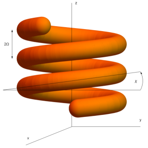
Figure 1: A schematic representation of a CSTF’s single helical column, with the structural period $2\Omega$ and inclination angle $\chi$ indicated.

A variety of materials can be used to make CSTFs [19] via physical vapor deposition [20, 21], with a range of periods $2\Omega$ and inclination angles $\chi$. Following Faryad et al. [11], for illustrative calculations let us choose $\epsilon_{a}=3.965$, $\epsilon_{b}=4.917$, $\epsilon_{c}=4.361$, $\chi=67.53^{\circ}$, $h=1$, and $\Omega=160$ nm for the CSTF. Furthermore, let us set $n_{s}=2.650+0.226i$ as the complex-valued refractive index of the isotropic dielectric material. This value of $n_{s}$ does not correspond precisely to any known natural material, as far as the authors are aware. However, a material with such a refractive index may be straightforwardly conceptualized as a homogenized composite material arising from readily-available natural component materials[22]. The free-space wavelength $\lambda_{\scriptscriptstyle 0}=633$ nm for all data reported here.

The following two theoretical problems have to be investigated: (a) a canonical boundary-value problem which yields a dispersion relation for the wavenumber $q$ of the Dyakonov–Tamm wave, and (b) a more realistic reflection–transmission problem which yields absorptance data.

(a) Canonical boundary-value problem. Suppose that the CSTF occupies the half-space $z<0$ while the isotropic dielectric material occupies the complementary half-space $z>0$. Following a standard procedure [1], Cartesian solutions to the frequency-domain Maxwell curl postulates are sought which decay as $z\to\pm\infty$ with the wavenumber $q$ being independent of $z$. The allowable values of $q$ arise as roots of a dispersion relation of the form ${\sf det}[{\underline{\underline{Y}}}(q)]=0$ where the matrix $[\underline{\underline{Y}}]$ is a function of $q$ and ${\sf det}$ denotes the determinant.

The scaled value of $\ln\left\{{\sf det}[{\underline{\underline{Y}}}(q)]\right\}$ is mapped in the complex $q$ plane in Fig. 2 for $\psi=30^{\circ}$. The values of $q$ are normalized relative to the free-space wavenumber $k_{\scriptscriptstyle 0}=2\pi/\lambda_{\scriptscriptstyle 0}$. Four roots of the dispersion relation may be deduced from Fig. 2. These are presented in Table 1 along with the respective values of the phase speed $v_{DT}=\omega/\mbox{Re}\left[q\right]$ relative to the phase speed in the bulk isotropic dielectric material, namely $v_{s}=\omega/k_{\scriptscriptstyle 0}\,\mbox{Re}\left[n_{s}\right]$, wherein $\omega$ is the angular frequency. For each of the four allowable values of $q$ for surface-wave propagation, the phase speed $v_{DT}$ exceeds $v_{s}$. Therefore, each solution identifies an HPSDT surface wave.

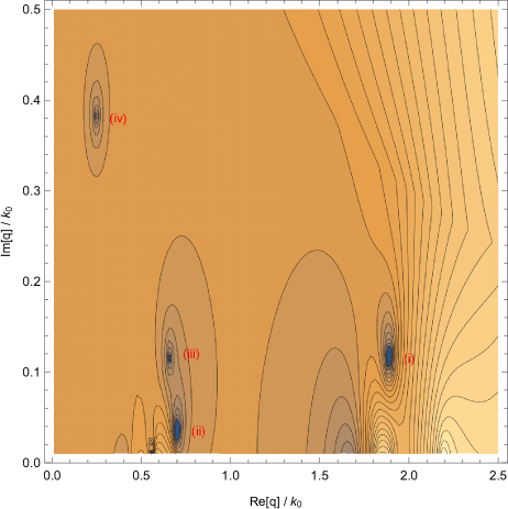
Figure 2: Scaled value of $\ln\left\{{\sf det}[{\underline{\underline{Y}}}(q)]\right\}$ mapped against Re$\left[q\right]/k_{\scriptscriptstyle 0}$ and Im$\left[q\right]/k_{\scriptscriptstyle 0}$ for $\psi=30^{\circ}$. The darkest regions contain the zeros of ${\sf det}[{\underline{\underline{Y}}}(q)]$. Solutions listed in Table 1 are indicated.

Table 1: Solutions of the dispersion relation for surface-wave propagation

Solution	$q/k_{\scriptscriptstyle 0}$	$v_{DT}/v_{s}$	$\sin^{-1}\left(\mbox{Re}\left[q\right]/k_{\scriptscriptstyle 0}\right)$
(i)	$1.90+{\color[rgb]{0,0,0}0.12i}$	1.39	$-$
(ii)	$0.70+0.04i$	3.78	$44.43^{\circ}$
(iii)	$0.65+0.12i$	4.08	$40.54^{\circ}$
(iv)	$0.25+0.38i$	10.60	$14.48^{\circ}$

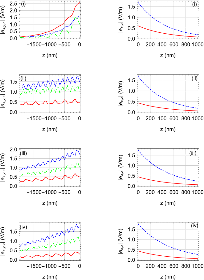
Figure 3: Spatial profiles of normalized magnitudes of the electric-field components in directions normal to the interface $z=0$ for solutions (i)–(iv) given in Table 1. The normalization procedure is described in Ref. 1. Key: $|e_{x}|$ blue dashed curves, $|e_{y}|$ green broken-dashed curves, $|e_{z}|$ red solid curves.

To explore this matter further, the spatial profiles of the absolute values of $\left\{e_{x},e_{y},e_{z}\right\}$ in directions normal to the interface are presented in Fig. 3 for each of the four solutions (i)–(iv) given in Table 1. These profiles reveal that the fields for each of the solutions (i)–(iv) are localized to the vicinity of the interface $z=0$, with the degree of localization being greater on the side of the isotropic dielectric material (i.e., $z>0$) than on the CSTF side (i.e., $z<0$). Since the CSTF is nondissipative, the decaying profiles in the $z<0$ half-space provide further evidence in support of the excitation of HPSDT surface waves.

Even though ${\rm Re}[q]<k_{\scriptscriptstyle 0}$ for solutions (ii)–(iv), these HPSDT surface waves cannot be classified as leaky surface waves. This is because both partnering materials occupy half spaces so that the issue of leakage cannot arise.

(b) Reflection–transmission problem. Suppose that the CSTF occupies the finitely thick region $-L_{CSTF}<z<0$ while the isotropic dielectric material occupies the finitely region $L_{s}>z>0$. The half spaces $z<-L_{CSTF}$ and $z>L_{s}$ are vacuous. An incident plane wave propagates in the half space $z<-L_{CSTF}$ towards the CSTF, with its wavevector oriented at the acute angle $\theta_{inc}$ to ${\mathbf{u}}_{z}$. Therefore, a reflected plane wave propagates in the half space $z<-L_{CSTF}$ away from the CSTF, with its wavevector oriented at the acute angle $\theta_{inc}$ to $-{\mathbf{u}}_{z}$; and a transmitted plane wave propagates in the half space $z>L_{s}$ away from the isotropic dielectric material, with its wavevector oriented at the acute angle $\theta_{inc}$ to ${\mathbf{u}}_{z}$.

In view of the structurally chiral morphology of the CSTF [19], let the incident plane wave be either left-circularly polarized (LCP) or right-circularly polarized (RCP). Also, given the rates of decay of the electric-field components evident in Fig. 3, let us choose $L_{CSTF}=1.28\,\mu$m (i.e., 40 CSTF periods) and $L_{s}=200$ nm. The procedure for solving the reflection–transmission problem and thereby computing the absorptances for LCP incident light, namely $\mathcal{A}_{L}$, and for RCP incident light, namely $\mathcal{A}_{R}$, is comprehensively described elsewhere [19]. Graphs of $\mathcal{A}_{L}$ and $\mathcal{A}_{R}$ plotted versus $\theta_{inc}$ are provided in Fig. 4. The $\theta_{inc}$-regime of relatively low values of $\mathcal{A}_{R}$ as compared to $\mathcal{A}_{L}$, apparent in Fig. 4 extending over the range $22^{\circ}\lessapprox\theta_{inc}\lessapprox 46^{\circ}$, is a manifestation of the circular Bragg phenomenon by which means the CSTF discriminates between incident LCP light and incident RCP light [19].

Values of the solution $q$ of the dispersion relation for the canonical boundary-value problem give an indication of the values of the angle of incidence $\theta_{inc}$ at which the excitation of HPSDT surface waves may be expected. Values of the angle of incidence are estimated as $\sin^{-1}\left(\mbox{Re}\left[q\right]/k_{\scriptscriptstyle 0}\right)$ and are listed in the rightmost column in Table 1. Solution (i) does not have a corresponding (real-valued) angle of incidence for the reflection–transmission problem, but solutions (ii)–(iv) do.

In Fig. 4 peaks in both $\mathcal{A}_{L}$ and $\mathcal{A}_{R}$ may be observed in the vicinity of the three angles of incidence inferred from solutions (ii)–(iv). This observation provides further evidence in support of the existence of HPSDT surface waves.

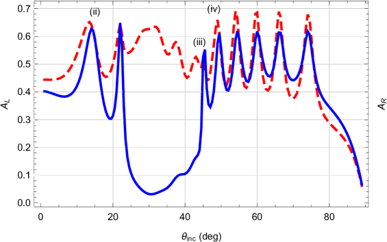
Figure 4: Absorptances $\mathcal{A}_{L}$ (red dashed curve) and $\mathcal{A}_{R}$ (blue solid curve) plotted against angle of incidence $\theta_{inc}$. Peaks corresponding to solutions (ii)–(iv) in Table 1 are labeled.

In conclusion, the two numerical studies presented here, one based on a canonical boundary-value problem and the other on a reflection–transmission problem, provide strong evidence of the existence high-phase-speed Dyakonov–Tamm surface waves that may be guided by the planar interface of a structurally chiral material and a dissipative isotropic dielectric material. For the specific example investigated, the given propagation direction supported the propagation of four HPSDT surface waves with each having a phase speed exceeding the phase speed of plane waves in isotropic partnering material. Furthermore, in the case of the most extreme solution, the phase speed of the Dyakonov–Tamm surface wave exceeded the phase speed in the bulk isotropic dielectric material by a factor of 10.

Lastly, the dissipative aspect of the isotropic dielectric material is not critical for the existence of HPSDT surface waves. Indeed, if the computations reported herein were repeated with the complex-valued refractive index $n_{s}$ replaced by the real-valued refractive index Re$\left[n_{s}\right]$, then qualitatively similar results would be obtained, albeit the decay of the field profiles in the $z>0$ half-space for the canonical boundary-value problem would be slower than the decay represented in Fig. 3.

Acknowledgment. AL is grateful to the Charles Godfrey Binder Endowment at Penn State for ongoing support of his research.

References

- [1] J. A. Polo Jr., T. G. Mackay, and A. Lakhtakia, Electromagnetic Surface Waves: A Modern Perspective, Elsevier, Waltham, MA (2013).
- [2] F. N. Marchevskiĭ, V. L. Strizhevskiĭ, and S. V. Strizhevskiĭ, “Singular electromagnetic waves in bounded anisotropic media,” Sov. Phys. Solid State 26(5), 911–912 (1984).
- [3] M. I. D’yakonov, “New type of electromagnetic wave propagating at an interface,” Sov. Phys. JETP 67(4), 714–716 (1988).
- [4] O. Takayama, L. Crasovan, D. Artigas, and L. Torner, “Observation of Dyakonov surface waves,” Phys. Rev. Lett. 102(4), 043903 (2009).
- [5] O. Takayama, L.-C. Crasovan, S. K. Johansen, D. Mihalache, D. Artigas, and L. Torner, “Dyakonov surface waves: a review,” Electromagnetics 28(3), 216–145 (2008).
- [6] P. Yeh, A. Yariv, and C.-S. Hong, “Electromagnetic propagation in periodic stratified media. I. General theory,” J. Opt. Soc. Am. 67(4), 423–438 (1977).
- [7] P. Yeh, A. Yariv, and A. Y. Cho, “Optical surface waves in periodic layered media,” Appl. Phys. Lett. 32(2), 104–105 (1978).
- [8] M. Shinn and W. M. Robertson, “Surface plasmon-like sensor based on surface electromagnetic waves in a photonic band-gap material,” Sens. Actuat. B: Chem. 105(2), 360–364 (2005).
- [9] A. Sinibaldi, N. Danz, E. Descrovi, P. Munzert, U. Schulz, F. Sonntag, L. Dominici, and F. Michelotti, “Direct comparison of the performance of Bloch surface wave and surface plasmon polariton sensors,” Sens. Actuat. B: Chem. 174(1), 292–298 (2012).
- [10] A. Lakhtakia and J. A. Polo Jr., “Dyakonov–Tamm wave at the planar interface of a chiral sculptured thin film and an isotropic dielectric material,” J. Eur. Opt. Soc.–Rapid Pubs. 2(1), 07021 (2007).
- [11] M. Faryad, A. Lakhtakia, and D. P. Pulsifer, “Dyakonov–Tamm waves guided by the planar interface of a chiral sculptured thin film,” J. Opt. Soc. Am. B 30(11), 3035–3040 (2013).
- [12] D. P. Pulsifer, M. Faryad, and A. Lakhtakia, “Observation of the Dyakonov–Tamm wave,” Phys. Rev. Lett. 111(24), 243902 (2013).
- [13] D. P. Pulsifer, M. Faryad, A. Lakhtakia, A. S. Hall, and L. Liu, “Experimental excitation of the Dyakonov–Tamm wave in the grating-coupled configuration,” Opt. Lett. 39(7), 2125–2128 (2013).
- [14] H. Maab, M. Faryad, and A. Lakhtakia, “Surface electromagnetic waves supported by the interface of two semi-infinite rugate filters with sinusoidal refractive-index profiles,” J. Opt. Soc. Am. B 28(5), 1204–1212 (2011).
- [15] A. Kavokin, I. Shelykh, and G. Malpuech, “Lossless interface modes at the boundary between two periodic dielectric structures,” Phys. Rev. B 72(23), 233102 (2005).
- [16] A. Kavokin, I. Shelykh, and G. Malpuech, “Optical Tamm states for the fabrication of polariton lasers,” Appl. Phys. Lett. 87(26), 261105 (2005).
- [17] I. V. Timofeev and S. Ya. Vetrov, “Chiral optical Tamm states at the boundary of the medium with helical symmetry of the dielectric tensor,” JETP Lett. 104(6), 380–383 (2016).
- [18] P. J. Collings, Liquid Crystals: Nature’s Delicate Phase of Matter, Princeton University Press, Princeton, NJ (1990).
- [19] A. Lakhtakia and R. Messier, Sculptured Thin Films: Nanoengineered Morphology and Optics, SPIE Press, Bellingham, WA (2005).
- [20] D.M. Mattox, The Foundations of Vacuum Coating Technology, Noyes Publications, Norwich, NY (2003).
- [21] I. J. Hodgkinson and Q. h. Wu, Birefringent Thin Films and Polarizing Elements, World Scientific, Singapore (1997).
- [22] T. G. Mackay and A. Lakhtakia, Modern Analytical Electromagnetic Homogenization, IoP Publishing, Bristol, UK (2015).