From a monotone probabilistic scheme to a probabilistic max-plus algorithm for solving Hamilton-Jacobi-Bellman equations

Abstract.

In a previous work (Akian, Fodjo, 2016), we introduced a lower complexity probabilistic max-plus numerical method for solving fully nonlinear Hamilton-Jacobi-Bellman equations associated to diffusion control problems involving a finite set-valued (or switching) control and possibly a continuum-valued control. This method was based on the idempotent expansion properties obtained by McEneaney, Kaise and Han (2011) and on the numerical probabilistic method proposed by Fahim, Touzi and Warin (2011) for solving some fully nonlinear parabolic partial differential equations. A difficulty of the algorithm of Fahim, Touzi and Warin is in the critical constraints imposed on the Hamiltonian to ensure the monotonicity of the scheme, hence the convergence of the algorithm. Here, we propose a new “probabilistic scheme” which is monotone under rather weak assumptions, including the case of strongly elliptic PDE with bounded coefficients. This allows us to apply our probabilistic max-plus method in more general situations. We illustrate this on the evaluation of the superhedging price of an option under uncertain correlation model with several underlying stocks and changing sign cross gamma, and consider in particular the case of 5 stocks leading to a PDE in dimension 5.

1. Introduction

We consider a finite horizon diffusion control problem on $\mathbb{R}^{d}$ involving at the same time a “discrete” control taking its values in a finite set $\mathcal{M}$, and a “continuum” control taking its values in some subset $\mathcal{U}$ of a finite dimensional space $\mathbb{R}^{p}$ (for instance a convex set with nonempty interior), which we next describe.

Let $T$ be the horizon. The state $\xi_{s}\in\mathbb{R}^{d}$ at time $s\in[0,T]$ satisfies the stochastic differential equation

(1) $$d\xi_{s}=f^{\mu_{s}}(\xi_{s},u_{s})ds+\sigma^{\mu_{s}}(\xi_{s},u_{s})dW_{s}\enspace,$$

where $(W_{s})_{s\geq 0}$ is a $d$-dimensional Brownian motion on a filtered probability space $(\Omega,\mathcal{F},(\mathcal{F}_{s})_{0\leq s\leq T},P)$. The control processes $\mu:=(\mu_{s})_{0\leq s\leq T}$ and $u:=(u_{s})_{0\leq s\leq T}$ take their values in the sets $\mathcal{M}$ and $\mathcal{U}$ respectively and they are admissible if they are progressively measurable with respect to the filtration $(\mathcal{F}_{s})_{0\leq s\leq T}$. We assume that, for all $m\in\mathcal{M}$, the maps $f^{m}:\mathbb{R}^{d}\times\mathcal{U}\to\mathbb{R}^{d}$ and $\sigma^{m}:\mathbb{R}^{d}\times\mathcal{U}\to\mathbb{R}^{d\times d}$ are continuous and satisfy properties implying the existence of the process $(\xi_{s})_{0\leq s\leq T}$ for any admissible control processes $\mu$ and $u$.

Given an initial time $t\in[0,T]$, the control problem consists in maximizing the following payoff:

$$J(t,x,\mu,u):= \mathbb{E}\left[\int_{t}^{T}e^{-\int_{t}^{s}\delta^{\mu_{\tau}}(\xi_{\tau},u_{\tau})d{\tau}}\ell^{\mu_{s}}(\xi_{s},u_{s})ds\right.$$

$$\left.\qquad+e^{-\int_{t}^{T}\delta^{\mu_{\tau}}(\xi_{\tau},u_{\tau})d{\tau}}\psi(\xi_{T})\mid\xi_{t}=x\right]\enspace,$$

where, for all $m\in\mathcal{M}$, $\ell^{m}:\mathbb{R}^{d}\times\mathcal{U}\to\mathbb{R}$, $\delta^{m}:\mathbb{R}^{d}\times\mathcal{U}\to\mathbb{R}$, and $\psi:\mathbb{R}^{d}\to\mathbb{R}$ are given continuous maps. We then define the value function of the problem as the optimal payoff:

$$v(t,x)=\sup_{\mu,u}J(t,x,\mu,u)\enspace,$$

where the maximization holds over all admissible control processes $\mu$ and $u$.

Let $\mathbb{S}_{d}$ denotes the set of symmetric $d\times d$ matrices and let us denote by $\leq$ the Loewner order on $\mathbb{S}_{d}$ ($A\leq B$ if $B-A$ is nonnegative). The Hamiltonian $\mathcal{H}:\mathbb{R}^{d}\times\mathbb{R}\times\mathbb{R}^{d}\times\mathbb{S}_{d}\to\mathbb{R}$ of the above control problem is defined as:

(2a) $$\mathcal{H}(x,r,p,\Gamma):= \max_{m\in\mathcal{M}}\mathcal{H}^{m}(x,r,p,\Gamma)\enspace,$$

with

(2b) $$\mathcal{H}^{m}(x,r,p,\Gamma):= \max_{u\in\mathcal{U}}\mathcal{H}^{m,u}(x,r,p,\Gamma)\enspace,$$

$$\mathcal{H}^{m,u}(x,r,p,\Gamma):= \frac{1}{2}\mathop{\mathrm{tr}}\left(\sigma^{m}(x,u)\sigma^{m}(x,u)^{\mathsf{T}}\,\Gamma\right)+f^{m}(x,u)\cdot p$$

(2c) $$\qquad-\delta^{m}(x,u)r+\ell^{m}(x,u)\enspace.$$

Under suitable assumptions, the value function $v:[0,T]\times\mathbb{R}^{d}\to\mathbb{R}$ is the unique (continuous) viscosity solution of the following Hamilton-Jacobi-Bellman equation

(3a) $$-\frac{\partial v}{\partial t}-\mathcal{H}(x,v(t,x),Dv(t,x),D^{2}v(t,x))=0,\quad x\in\mathbb{R}^{d},\;t\in[0,T),$$

(3b) $$v(T,x)=\psi(x),\quad x\in\mathbb{R}^{d},$$

satisfying also some growth condition at infinity (in space).

In [6], Fahim, Touzi and Warin proposed a probabilistic numerical method to solve such fully nonlinear partial differential equations (3), inspired by their backward stochastic differential equation interpretation given by Cheridito, Soner, Touzi and Victoir in [5]. In [6], the convergence of the resulting algorithm follows from the theorem of Barles and Souganidis [3], which requires the monotonicity of the scheme. Moreover, for this monotonicity to hold, critical constraints are imposed on the Hamiltonian: the diffusion matrices $\sigma^{m}(x,u)\sigma^{m}(x,u)^{\mathsf{T}}\,$ need at the same time to be bounded from below (with respect to the Loewner order) by a symmetric positive definite matrix $a$ and bounded from above by $(1+2/d)a$. Such a constraint can be restrictive, in particular it may not hold even when the matrices $\sigma^{m}(x,u)$ do not depend on $x$ and $u$ but take different values for $m\in\mathcal{M}$. In [7], Guo, Zhang and Zhuo proposed a monotone scheme exploiting the diagonal part of the diffusion matrices and combining a usual finite difference scheme to the scheme of [6]. This new scheme can be applied in more general situations than the one of [6], but still does not work for general control problems.

McEneaney, Kaise and Han proposed in [8, 11] an idempotent numerical method which works at least when the Hamiltonians with fixed discrete control, $\mathcal{H}^{m}$, correspond to linear quadratic control problems. This method is based on the distributivity of the (usual) addition operation over the supremum (or infimum) operation, and on a property of invariance of the set of quadratic forms. It computes in a backward manner the value function $v(t,\cdot)$ at time $t$ as a supremum of quadratic forms. However, as $t$ decreases, the number of quadratic forms generated by the method increases exponentially (and even become infinite if the Brownian is not discretized in space) and some pruning is necessary to reduce the complexity of the algorithm.

In [1], we introduced an algorithm combining the two above methods which uses in particular the simulation of as many uncontrolled stochastic processes as discrete controls. Moreover, we shown that even without pruning, the complexity of the algorithm is bounded polynomially in the number of discretization time steps and the sampling size.

However, due to the above critical constraints imposed in [6], the algorithm of [1] is difficult to apply in practical situations. One way to avoid these critical constraints, is as suggested in [1], to introduce a large number of Hamiltonians $\mathcal{H}^{m}$ such that each of them satisfy the constraints. Since one need to simulate a stochastic process for each Hamiltonian, this technique may increase the complexity unnecessarily.

Here, we propose a different probabilistic discretization of the Hessian of the value function, which ensures the monotonicity of the scheme in rather general situations, including the case of strongly elliptic PDE with bounded coefficients and we show how the algorithm of [1] associated to the new scheme can be applied in these situations and high dimension.

The paper is organized as follows. In Section 2, we recall the scheme of [6]. Then, the new monotone probabilistic discretization is presented in Section 3. In Section 4, we recall the algorithm of [1] and show how it can be combined with the scheme of Section 3. In Section 5, we illustrate this algorithm numerically. There, we consider the evaluation of the superhedging price of an option under uncertain correlation model with several underlying stocks and changing sign cross gamma. We consider in particular the case of 5 stocks leading to a PDE in dimension 5.

2. The probabilistic method of Fahim, Touzi and Warin

In the present section we recall the probabilistic numerical method of Fahim, Touzi and Warin proposed in [6]. We begin with the general description and continue with an example in order to illustrate the critical constraint.

2.1. General description

Let $h$ be a time discretization step such that $T/h$ is an integer. We denote by $\mathcal{T}_{h}=\{0,h,2h,\ldots,T-h\}$ the set of discretization times of $[0,T)$. Let $\mathcal{H}$ be any Hamiltonian of the form (2). Let us decompose $\mathcal{H}$ as the sum $\mathcal{H}=\mathcal{L}+\mathcal{G}$ of the (linear) generator $\mathcal{L}$ of a given diffusion (with no control) and of a nonlinear elliptic Hamiltonian $\mathcal{G}$. This means that

$$\mathcal{L}(x,p,\Gamma):= \frac{1}{2}\mathop{\mathrm{tr}}\left(a(x)\Gamma\right)+\underline{f}(x)\cdot p\enspace,$$

with $a(x)=\underline{\sigma}(x)\underline{\sigma}(x)^{\mathsf{T}}\,$, for some drift map $x\in\mathbb{R}^{d}\mapsto\underline{f}(x)\in\mathbb{R}^{d}$ and standard deviation (volatility) map $x\in\mathbb{R}^{d}\mapsto\underline{\sigma}(x)\in\mathbb{R}^{d\times d}$. This also means that the Hamiltonian $\mathcal{G}=\mathcal{H}-\mathcal{L}$ satisfies the ellipticity condition, that is $\partial_{\Gamma}{\mathcal{G}}(x,r,p,\Gamma)$ is positive semidefinite, for all $x\in\mathbb{R}^{d},\;r\in\mathbb{R},p\in\mathbb{R}^{d},\Gamma\in\mathbb{S}_{d}$. We shall also assume that $a(x)$ is positive definite (which implies that $\underline{\sigma}(x)$ is invertible). A typical example is obtained when $\mathcal{H}$ is uniformly strongly elliptic and $\mathcal{L}(x,p,\Gamma)=\frac{\epsilon}{2}\mathop{\mathrm{tr}}\left(\Gamma\right)$ with $\epsilon$ small enough, which corresponds to the generator $\frac{\epsilon}{2}\Delta v$. Denote by $\hat{X}$ the Euler discretization of the diffusion with generator $\mathcal{L}$:

(4) $$\hat{X}(t+h)=\hat{X}(t)+\underline{f}(\hat{X}(t))h+\underline{\sigma}(\hat{X}(t))(W_{t+h}-W_{t})\enspace.$$

The time discretization of (3) proposed in [6] has the following form:

(5) $$v^{h}(t,x)=T_{t,h}(v^{h}(t+h,\cdot))(x),\quad t\in\mathcal{T}_{h}\enspace,$$

with

(6) $$T_{t,h}(\phi)(x)=\mathcal{D}_{t,h}^{0}(\phi)(x)+h\mathcal{G}(x,\mathcal{D}_{t,h}^{0}(\phi)(x),\mathcal{D}_{t,h}^{1}(\phi)(x),\mathcal{D}_{t,h}^{2}(\phi)(x))\enspace.$$

In (6), $\mathcal{D}_{t,h}^{i}(\phi)$, $i=0,1,2$, denotes the following approximation of the $i$th differential of $e^{h\mathcal{L}}\phi$:

(7a) $$\mathcal{D}_{t,h}^{i}(\phi)(x) =\mathbb{E}(D^{i}\phi(\hat{X}(t+h))\mid\hat{X}(t)=x)\enspace,$$

where $$D^{i} i$$ denotes the th differential operator. Moreover, it is computed using the following scheme:

(7b) $$\mathcal{D}_{t,h}^{i}(\phi)(x) =\mathbb{E}(\phi(\hat{X}(t+h))\mathcal{P}^{i}_{t,x,h}(W_{t+h}-W_{t})\mid\hat{X}(t)=x)\enspace,$$

where, for all $t,x,h,i$, $\mathcal{P}^{i}_{t,x,h}$ is the polynomial of degree $i$ in the variable $w\in\mathbb{R}^{d}$ given by:

(8a) $$\mathcal{P}^{0}_{t,x,h}(w) =1\enspace,$$

(8b) $$\mathcal{P}^{1}_{t,x,h}(w) =(\underline{\sigma}(x)^{\mathsf{T}}\,)^{-1}h^{-1}w\enspace,$$

(8c) $$\mathcal{P}^{2}_{t,x,h}(w) =(\underline{\sigma}(x)^{\mathsf{T}}\,)^{-1}h^{-2}(ww^{\mathsf{T}}\,-hI)(\underline{\sigma}(x))^{-1}\enspace,$$

where $I$ is the $d\times d$ identity matrix. Note that the equality between the two formulations in (7) holds for all $\phi$ with exponential growth [6, Lemma 2.1].

In addition to the formal expression in (6-8), which can be compared to a standard numerical approximation (or more precisely to a time discretization), the method of [6] includes the approximation of the conditional expectations in (7) by any probabilistic method such as a regression estimator: after a simulation of the processes $W_{t}$ and $\hat{X}(t)$, one apply at each time $t\in\mathcal{T}_{h}$ a regression estimation to find the value of $\mathcal{D}_{t,h}^{i}(v^{h}(t+h,\cdot))$ at the points $\hat{X}(t)$ by using the values of $v^{h}(t+h,\hat{X}(t+h))$ and $W_{t+h}-W_{t}$. Hence, although in our setting the operator $T_{t,h}$ does not depend on $t$, since both the law of $W_{t+h}-W_{t}$ and the Hamiltonian $\mathcal{H}$ do not depend on $t$, we shall keep the index $t$ in the above expressions to allow further approximations as above.

In [6], the convergence of the time discretization scheme (5) is proved by using the theorem of Barles and Souganidis of [3], under the above assumptions together with the critical assumption that $\partial_{\Gamma}{\mathcal{G}}(x,r,p,\Gamma)$ is lower bounded by some positive definite matrix (for all $x\in\mathbb{R}^{d},\;r\in\mathbb{R},p\in\mathbb{R}^{d},\Gamma\in\mathbb{S}_{d}$) and that $\mathop{\mathrm{tr}}(a(x)^{-1}\partial_{\Gamma}{\mathcal{G}})\leq 1$. Indeed, the latter conditions together with the boundedness of $\partial_{p}{\mathcal{G}}$ are used to show (in Lemma 3.12 and 3.14) that the operator $T_{t,h}$ is a $Ch$-almost monotone operator over the set of Lipschitz continuous functions from $\mathbb{R}^{d}$ to $\mathbb{R}$, where we shall say that an operator $T$ between any partially ordered sets $\mathcal{F}$ and $\mathcal{F}^{\prime}$ of real valued functions (for instance $\mathbb{R}^{n}$, or the set of bounded functions from some set $\Omega$ to $\mathbb{R}$) is $L$-almost monotone, for some constant $L\geq 0$, if

(9) $$\phi,\psi\in\mathcal{F},\;\phi\leq\psi\implies T(\phi)\leq T(\psi)+L\sup(\psi-\phi)\enspace,$$

and that it is monotone, when this holds for $L=0$.

Note that some other technical assumptions are used in [6], such as the uniform Lipschitz continuity of the Hamiltonian $\mathcal{H}$, and the boundedness of the value function of the corresponding control problem, which are less crucial, since they can be replaced by more usual stochastic control assumptions (like boundedness and Lipschitz continuity of the coefficients of the controlled diffusion itself).

In [1], we proposed to bypass the critical constraint, by assuming that the Hamiltonians $\mathcal{H}^{m}$ (but not necessarily $\mathcal{H}$) satisfy the critical constraint, and applying the above scheme to the Hamiltonians $\mathcal{H}^{m}$. Another way is to replace the $\mathcal{G}$ part of the operator (6) by any approximation of it in $O(h)$, for instance by using or combining the probabilistic scheme with a finite difference scheme, as is done in [7]. Indeed, the operator (6) is already an approximation of the semigroup of the HJB equation in time $h$ which is at best in $O(h^{2})$, therefore one can replace, with no loss of order of approximation, the $\mathcal{D}_{t,h}^{i}(\phi)$ inside $\mathcal{G}$ by $D^{i}\phi(x)$ (which is an approximation in $O(h)$) or any approximation of order $O(h)$ of it. Note however that the first $\mathcal{D}_{t,h}^{0}(\phi)$ in (6) can only be replaced by an approximation in $O(h^{2})$ or at least in $o(h)$. In Section 3, we shall propose an approximation of $\mathcal{D}_{t,h}^{2}(\phi)$ or $D^{2}\phi(x)$ which is expressed as a conditional expectation as in (7b), and leads to a monotone operator $T_{t,h}$ without assuming the critical constraint. The advantage with respect to finite difference methods or with the method of [7] is that it can still be used with simulations. Before describing the new scheme, we shall compare on some examples the method of [6] with finite difference schemes.

2.2. Examples and comparison with finite difference schemes constraints

Let us first show on examples the behavior of the discretization of [6]. This should help to understand the advantage of the new discretization that we propose in next section. For this, we shall show what happen when the increments of the Brownian motion $W_{t+h}-W_{t}$ are replaced by any finite valued independent random variables with same law. This allows one in particular to compare the discretization of [6] with finite difference schemes. Similar comparisons were done in [6] but here we shall discuss in addition the meaning of the critical constraint in this situation.

To simplify the comparison, consider the case where $\mathcal{H}$ is linear and depends only on $\Gamma$, that is

$$\mathcal{H}(x,r,p,\Gamma)=\frac{1}{2}\mathop{\mathrm{tr}}\left(A\Gamma\right)$$

where $A$ is a $d$-dimensional symmetric positive definite matrix. We assume that $A\geq I$ and choose $\mathcal{L}(x,p,\Gamma)=\frac{1}{2}\mathop{\mathrm{tr}}\left(\Gamma\right)$, that is $\underline{f}\equiv 0$ and $\underline{\sigma}\equiv I$. Hence, $\mathcal{G}(x,r,p,\Gamma)=\frac{1}{2}\mathop{\mathrm{tr}}\left((A-I)\Gamma\right)$.

Then, denoting by $N$ any $d$-dimensional normal random variable, we get that the operator $T_{t,h}$ of (6) satisfies:

$$T_{t,h}(\phi)(x) =\mathcal{D}_{t,h}^{0}(\phi)(x)+h\frac{1}{2}\mathop{\mathrm{tr}}((A-I)\mathcal{D}_{t,h}^{2}(\phi)(x)))$$

(10) $$=\mathbb{E}\left(\phi(x+\sqrt{h}N)(1+\frac{1}{2}\mathop{\mathrm{tr}}((A-I)(NN^{\mathsf{T}}\,-I)))\right)\enspace.$$

This operator is linear, and it is thus monotone if and only if for almost all values of $N$ the coefficient of $\phi(x+\sqrt{h}N)$ inside the expectation, that is $(1+\frac{1}{2}\mathop{\mathrm{tr}}((A-I)(NN^{\mathsf{T}}\,-I)))$, is nonnegative. The critical constraint $\mathop{\mathrm{tr}}(a(x)^{-1}\partial_{\Gamma}{\mathcal{G}})\leq 1$ is equivalent here to $\frac{1}{2}\mathop{\mathrm{tr}}(A-I)\leq 1$. This corresponds exactly to the condition that the coefficient of $\phi(x)$ inside the expectation is nonnegative. Thus, if $N$ is replaced by any random variable taking a finite number of values including $0$, the critical constraint is necessary.

Consider the dimension $d=1$ and a simple discretization of $N$ by the random variable taking the values $\pm\nu$ with probability $1/(2\nu^{2})$ and the value $0$ with probability $1-1/\nu^{2}$, where $\nu>1$. Then, we obtain

(11) $$T_{t,h}(\phi)(x)=\phi(x)+\frac{b}{2\nu^{2}}\left(\phi(x+\sqrt{h}\nu)+\phi(x-\sqrt{h}\nu)-2\phi(x)\right)\enspace,$$

with $b=1+\frac{1}{2}(A_{11}-1)(\nu^{2}-1)$. This scheme is equivalent to an explicit finite difference discretization of (3) with a space step $\Delta x=\sqrt{h}\nu$. However it is consistent with the Hamilton-Jacobi-Bellman equation (3) if and only if $b=A_{11}$ and so if and only if $\nu=\sqrt{3}$. In that case, the critical condition $\frac{1}{2}(A_{11}-1)\leq 1$ is necessary for the scheme to be monotone and it is equivalent to the CFL condition $A_{11}h\leq(\Delta x)^{2}$.

For finite difference schemes, the CFL condition can be satisfied by increasing $\Delta x$. However, here $\Delta x$ is strongly connected to the possible values of $N$ and since the probability of large $N$ is small, one cannot avoid the critical constraint if we keep the discretization (7b) of $\mathcal{D}_{t,h}^{2}(\phi)(x)$.

Let us consider now the same example in dimension $2$. In that case, the usual difficulty of finite difference schemes is in the monotone discretization of mixed derivatives. This can be solved for instance when the matrix $A$ is diagonally dominant by using only close points to the initial point of the grid, that is using the 9-points stencil, see [10], or in general by using points of the grid which are far from the initial point (see for instance [4, 12]). Here, we shall see that this difficulty is hidden by the critical constraint $\frac{1}{2}\mathop{\mathrm{tr}}(A-I)\leq 1$, which implies in particular that the matrix $A$ is diagonally dominant.

Indeed, consider the simple discretization of $N$ where each entry of $N=(N_{i})_{i=1,\ldots,2}$ is replaced by a random variable as above, taking the values $\pm\sqrt{3}$ with probability $1/6$ and the value $0$ with probability $2/3$. In that case, the critical constraint $\frac{1}{2}(A_{11}+A_{22}-2)\leq 1$ is necessary and sufficient for the discretization to be monotone. We have

$$T_{t,h}(\phi)(x)= \mathbb{E}\left(\phi(x+\sqrt{h}N)(1+\frac{1}{2}\sum_{i,j=1}^{2}(A_{ij}-\delta_{ij})(N_{i}N_{j}-\delta_{ij}))\right)$$

$$= \phi(x)\frac{2}{9}(2-\mathop{\mathrm{tr}}(A-I))$$

$$+\frac{1}{18}\sum_{i=1}^{2}\sum_{\epsilon=\pm 1}\left(\phi(x+\sqrt{3h}\epsilon e_{i})(3(A_{ii}-1)+2-\mathop{\mathrm{tr}}(A-I))\right)$$

$$+\frac{1}{72}\sum_{\epsilon_{1}=\pm 1,\epsilon_{2}=\pm 1}\Big{(}\phi(x+\sqrt{3h}(\epsilon_{1}e_{1}+\epsilon_{2}e_{2}))$$

$$\qquad\Big{(}3\Big{(}\sum_{i,j=1}^{2}(A_{ij}-\delta_{ij})\epsilon_{i}\epsilon_{j}\Big{)}+2-\mathop{\mathrm{tr}}(A-I)\Big{)}\Big{)}\enspace.$$

where $(e_{1},e_{2})$ is the canonical basis of $\mathbb{R}^{2}$. This discretization can be rewritten as

$$T_{t,h}(\phi)(x)= \phi(x)+\frac{h}{2}\left(\left(\sum_{i,j=1}^{2}(A_{ij}-\delta_{ij}b)D_{ij}^{h}\phi(x)\right)+b\Delta^{h}\phi(x)\right)\enspace,$$

where $b=(1+\mathop{\mathrm{tr}}(A-I))/3$, $D_{ij}^{h}\phi$ is the standard $5$-point stencil discretization of the partial derivative $\frac{\partial^{2}\phi}{\partial x_{i}\partial x_{j}}$ on the grid with space step $\Delta x=\sqrt{3h}$ (as above), and $\Delta^{h}\phi$ is the discretization of $\Delta\phi$ using the external vertices of the $9$-point stencil (that is the points $x+\Delta x(\pm e_{1}+\pm e_{2})$). Note also that the critical constraint $\mathop{\mathrm{tr}}(A-I)\leq 2$ implies $b\leq 1$. Moreover, since $A-I$ is positive semidefinite, then $2|A_{12}|\leq\mathop{\mathrm{tr}}(A-I)\leq 2$ and $A_{ii}\geq 1$, so $|A_{12}|\leq A_{ii}$ for $i=1,2$. The latter condition means that the matrix is diagonally dominant. So, in dimension $2$, the critical constraint implies automatically that the equation can be discretized using a 9-points stencil finite difference monotone scheme.

Hence, the difficulty of the probabilistic scheme does not come only or necessarily from mixed derivatives as for finite difference schemes. It essentially comes from the weights of the possible values of $N$, which link strongly the possible space discretization and time discretization steps. The new approximation of $\mathcal{D}_{t,h}^{2}(\phi)$ that we propose in next section will allows one to change these weights, while keeping the probabilistic interpretation.

3. A monotone probabilistic scheme for fully nonlinear PDEs

We denote by $\mathcal{C}^{k}$ the set of functions from $[0,T]\times\mathbb{R}^{d}$ to $\mathbb{R}$ with continuous partial derivatives up to order $k$ in $t$ and $x$, and by $\mathcal{C}^{k}_{\text{b}}$ the subset of functions with bounded such derivatives.

Theorem 3.1.

Let $v\in\mathcal{C}^{4}_{\text{b}}$, $\hat{X}$ as in (4), $\Sigma\in\mathbb{R}^{d\times\ell}$ for some $\ell$ and denote $A=\Sigma\Sigma^{\mathsf{T}}\,$. Let $N$ be a one dimensional normal random variable. For a nonnegative integer $k$, consider the polynomial $\mathcal{P}_{\Sigma,k}$ of degree $4k+2$ in the variable $w\in\mathbb{R}^{d}$ defined by:

(12a) $$\mathcal{P}_{\Sigma,k}(w)=c_{k}\sum_{j=1}^{\ell}([\Sigma^{\mathsf{T}}\,w]_{j})^{4k+2}\|\Sigma_{.j}\|_{2}^{-4k}-K$$

where, for any real vector $$v\in\mathbb{R}^{d} j\leq d [v]_{j} j v \Sigma\in\mathbb{R}^{d\times\ell} j\leq\ell \Sigma_{.j} j \Sigma$$ and , denotes the th coordinate of , for any matrix and , denotes the th column of , and

(12b) $$c_{k}=\frac{1}{\mathbb{E}\left[N^{4k+4}-N^{4k+2}\right]}\enspace,\qquad K:=\frac{\mathop{\mathrm{tr}}(A)}{4k+2}=\frac{\sum_{j=1}^{\ell}\|\Sigma_{.j}\|_{2}^{2}}{4k+2}\enspace.$$

We have, for $(t,x)\in[0,T]\times\mathbb{R}^{d}$:

(13) $$\mathbb{E}\left[\mathcal{P}_{\Sigma,k}(h^{-1/2}(W_{t+h}-W_{t}))\mid\hat{X}(t)=x\right]=0$$

$$h^{-1}\mathbb{E}\left[v(t+h,\hat{X}(t+h))\mathcal{P}_{\Sigma,k}(h^{-1/2}(W_{t+h}-W_{t}))\mid\hat{X}(t)=x\right]=$$

(14) $$\frac{1}{2}\mathop{\mathrm{tr}}(\underline{\sigma}(x)\Sigma\Sigma^{\mathsf{T}}\,\underline{\sigma}^{\mathsf{T}}\,(x)\,D^{2}v(t,x))+O(h)\enspace,$$

where the error $O(h)$ is uniform in $t$ and $x$.

Sketch of proof.

Since $\Sigma\Sigma^{\mathsf{T}}\,=\sum_{j=1}^{\ell}\Sigma_{.j}\Sigma_{.j}^{\mathsf{T}}\,$, it is sufficient to show (14) when $A=\Sigma_{.j}\Sigma_{.j}^{\mathsf{T}}\,$ for each $j=1,\ldots,\ell$. In that case, with $j$ fixed, using a unitary matrix $U$ with $j$th column equal to $\Sigma_{.j}/\|\Sigma_{.j}\|_{2}$, we obtain that (13-14) are equivalent to the same equations for $A=U_{.j}U_{.j}^{\mathsf{T}}\,$. Since $U$ is a unitary matrix, $U^{\mathsf{T}}\,(h^{-1/2}(W_{t+h}-W_{t}))$ is a $d$-dimensional normal random vector, and in particular its $j$th coordinate $[U^{\mathsf{T}}\,(h^{-1/2}(W_{t+h}-W_{t}))]_{j}$ is a normal random variable. This implies in particular (13). Applying a Taylor expansion of $v$ around $(t,x)$ up to order $2$ and using the values of the moments of any $d$-dimensional normal random vector, we deduce (14). ∎

Since the above approximation depends on the matrix to which the second derivative is multiplied, we cannot apply it directly as an argument of $\mathcal{G}$ as in (6), but need instead to use the expression of $\mathcal{G}$ as a supremum of Hamiltonians which are affine with respect to $r,p,\Gamma$ and apply (14) to each of these Hamiltonians. In what follows, we shall present a scheme which combine at the same time this idea and the one of [1]. Note that the decomposition of the matrix involved in the expression of the second order terms of the Hamiltonians as the product $A=\Sigma\Sigma^{\mathsf{T}}\,$ is used in a similar way to obtain general monotone finite difference discretizations (see for instance [12]).

Let us decompose the Hamiltonian $\mathcal{H}^{m,u}$ of (2c) as $\mathcal{H}^{m,u}=\mathcal{L}^{m}+\mathcal{G}^{m,u}$ with

$$\mathcal{L}^{m}(x,p,\Gamma):= \frac{1}{2}\mathop{\mathrm{tr}}\left(a^{m}(x)\Gamma\right)+\underline{f}^{m}(x)\cdot p\enspace,$$

and $a^{m}(x)=\underline{\sigma}^{m}(x)\underline{\sigma}^{m}(x)^{\mathsf{T}}\,$, and denote by $\hat{X}^{m}$ the Euler discretization of the diffusion with generator $\mathcal{L}^{m}$. Note that, we can also choose a linear operator $\mathcal{L}^{m}$ depending on $u$, but this would increase too much the number of simulations. We can also choose the same linear operator $\mathcal{L}^{m}$ for different values of $m$, which is the case in Algorithm 4.4 below. Assume that $a^{m}(x)$ is positive definite (so that $\underline{\sigma}^{m}(x)$ is invertible) and that $a^{m}(x)\leq\sigma^{m}(x,u)\sigma^{m}(x,u)^{\mathsf{T}}\,$, for all $x\in\mathbb{R}^{d},\;u\in\mathcal{U}$, and denote by $\Sigma^{m}(x,u)$ any $d\times\ell$ matrix such that

(15) $$\sigma^{m}(x,u)\sigma^{m}(x,u)^{\mathsf{T}}\,-a^{m}(x)=\underline{\sigma}^{m}(x)\Sigma^{m}(x,u)\Sigma^{m}(x,u)^{\mathsf{T}}\,\underline{\sigma}^{m}(x)^{\mathsf{T}}\,\enspace.$$

Such a matrix $\Sigma^{m}(x,u)$ exists under the above assumptions since $\underline{\sigma}^{m}(x)$ is invertible, and $\underline{\sigma}^{m}(x)^{-1}(\sigma^{m}(x,u)\sigma^{m}(x,u)^{\mathsf{T}}\,-a^{m}(x))(\underline{\sigma}^{m}(x))^{\mathsf{T}}\,)^{-1}$ is a symmetric nonnegative matrix. Indeed, one can choose $\Sigma^{m}(x,u)$ as the square root of the latter matrix. One may also use its Cholesky factorization in which zero columns are eliminated: this leads to a rectangular and triangular matrix $\Sigma^{m}(x,u)$ of size $d\times\ell$, where $\ell$ is the rank of the factorized matrix. This is what we use in the practical implementation of Algorithm 4.4 below.

Define

(16) $$\mathcal{G}^{m,u}_{1}(x,r,p):=(f^{m}(x,u)-\underline{f}^{m}(x))\cdot p-\delta^{m}(x,u)r+\ell^{m}(x,u)\enspace,$$

so that

$$\mathcal{G}^{m,u}(x,r,p,\Gamma)=\mathcal{G}^{m,u}_{1}(x,r,p)+\frac{1}{2}\mathop{\mathrm{tr}}\left(\underline{\sigma}^{m}(x)\Sigma^{m}(x,u)\Sigma^{m}(x,u)^{\mathsf{T}}\,\underline{\sigma}^{m}(x)^{\mathsf{T}}\,\Gamma\right)\enspace.$$

Applying (14) and (7), we deduce the following result.

Corollary 3.2.

Let $\mathcal{D}_{t,h,m}^{i}(\phi)$, $i=0,1$, be given by (7-8), with $\underline{\sigma}^{m}$ and $\hat{X}^{m}$ instead of $\underline{\sigma}$ and $\hat{X}$ respectively. Let $\mathcal{D}_{t,h,m,\Sigma,k}^{2}(\phi)$ be defined as:

$$\mathcal{D}_{t,h,m,\Sigma,k}^{2}(\phi)(x):=h^{-1}\mathbb{E}\left[\phi(\hat{X}^{m}(t+h))\mathcal{P}_{\Sigma,k}(h^{-1/2}(W_{t+h}-W_{t}))\mid\hat{X}^{m}(t)=x\right]$$

with $\mathcal{P}_{\Sigma,k}$ as in (12).

Consider the operator:

$$T_{t,h}(\phi)(x)=\max_{m\in\ M}\big{\{}\mathcal{D}_{t,h,m}^{0}(\phi)(x)$$

$$+h\max_{u\in\mathcal{U}}\big{(}\mathcal{G}_{1}^{m,u}(x,\mathcal{D}_{t,h,m}^{0}(\phi)(x),\mathcal{D}_{t,h,m}^{1}(\phi)(x))+\mathcal{D}_{t,h,m,\Sigma^{m}(x,u),k}^{2}(\phi)(x)\big{)}\big{\}}\enspace.$$

Assume that the maps $\sigma^{m}$, $f^{m}$ and $\Sigma^{m}$ are bounded with respect to $u\in\mathcal{U}$. Then, for $v\in\mathcal{C}^{4}_{\text{b}}$, $t\in\mathcal{T}_{h}$, and $x\in\mathbb{R}^{d}$, we have

$$\frac{T_{t,h}(v(t+h,\cdot))(x)-v(t,x)}{h}=\frac{\partial v}{\partial t}+\mathcal{H}(x,v(t,x),Dv(t,x),D^{2}v(t,x))+O(h)\enspace.$$

This result shows the consistency of the scheme (5) in the sense of [3]. This implies easily that if the solution $v$ of (3) is smooth enough, then the solution of (5) converges to $v$ when $h$ goes to zero. In the general case, when $v$ is only Lipschitz continuous for instance, the convergence is obtained by the theorem of Barles and Souganidis [3]. For this, one need to satisfy also the other assumptions of the theorem, that we shall now show.

Note that when $k=0$, and $\mathcal{L}^{m}=\mathcal{L}$ does not depend on $m$, the above operator $T_{t,h}$ coincides with the operator (6) proposed in [6], since $\mathcal{D}_{t,h,m,\Sigma,0}^{2}(\phi)(x)=\frac{1}{2}\mathop{\mathrm{tr}}(\underline{\sigma}(x)\Sigma\Sigma^{\mathsf{T}}\,\underline{\sigma}^{\mathsf{T}}\,(x)\,\mathcal{D}_{t,h}^{2}(\phi)(x))$. In [6, Lemma 3.12], the monotonicity of the scheme is proved under the critical constraint that $\mathop{\mathrm{tr}}(a(x)^{-1}\partial_{\Gamma}{\mathcal{G}})\leq 1$. This constraint is equivalent to the condition that $\frac{1}{2}\mathop{\mathrm{tr}}(\Sigma^{m}(x,u)\Sigma^{m}(x,u)^{\mathsf{T}}\,)\leq 1$ for all $x\in\mathbb{R}^{d}$ and all useful controls $m\in\mathcal{M}$ and $u\in\mathcal{U}$ that are optimal in the expression of $\mathcal{H}$, which means that the constant $K$ in Theorem 3.1 is $\leq 1$ for $k=0$. By increasing $k$, we can obtain that this constant $K$ is $\leq 1$ in more general situations, which implies the following monotonicity result.

Theorem 3.3.

Let $T_{t,h}$ be as in Corollary 3.2. Assume that the map $\mathop{\mathrm{tr}}(\Sigma^{m}(x,u)\Sigma^{m}(x,u)^{\mathsf{T}}\,)$ is upper bounded in $x$ and $u$ and let $\bar{a}$ be an upper bound. Assume also that $\delta^{m}$ is upper bounded, and that there exists a bounded map $g^{m}$ (in $x$ and $u$) such that $f^{m}(x,u)-\underline{f}^{m}(x)=\underline{\sigma}(x)\Sigma^{m}(x,u)g^{m}(x,u)$. Then, for $k$ such that $\bar{a}<4k+2$, there exists $h_{0}$ such that $T_{t,h}$ is monotone for $h\leq h_{0}$ over the set of bounded continuous functions $\mathbb{R}^{d}\to\mathbb{R}$, and there exists $C>0$ such that $T_{t,h}$ is $Ch$-almost monotone for all $h>0$.

Proof.

Let $\phi,\psi:\mathbb{R}^{d}\to\mathbb{R}$ be bounded and let $h>0$. We can write $T_{t,h}$ as the supremum over $m\in\mathcal{M}$ and $u\in\mathcal{U}$ of the operators

$$T_{t,h}^{m,u}(\phi)(x)=\; \mathcal{D}_{t,h,m}^{0}(\phi)(x)$$

$$+h\big{(}\mathcal{G}_{1}^{m,u}(x,\mathcal{D}_{t,h,m}^{0}(\phi)(x),\mathcal{D}_{t,h,m}^{1}(\phi)(x))+\mathcal{D}_{t,h,m,\Sigma^{m}(x,u),k}^{2}(\phi)(x)\big{)}$$

$$=\; \mathbb{E}\left[\phi(\hat{X}^{m}(t+h))\mathcal{P}^{h,m,u,x}(h^{-1/2}(W_{t+h}-W_{t}))\mid\hat{X}^{m}(t)=x\right]$$

$$+h\ell^{m}(x,u)\enspace,$$

where

$$\mathcal{P}^{h,m,u,x}(w)= 1+h(f^{m}(x,u)-\underline{f}^{m}(x))\cdot((\underline{\sigma}(x)^{\mathsf{T}}\,)^{-1}h^{-1/2}w)$$

$$-h\delta^{m}(x,u)+\mathcal{P}_{\Sigma^{m}(x,u),k}(w)\enspace.$$

If $L\geq 0$ is such that $-L$ is a lower bound of $\mathcal{P}^{h,m,u,x}(w)$ for all $m,u,x,w$, we obtain that the operators $T_{t,h}^{m,u}$ satisfy (9), and taking the supremum, we get that $T_{t,h}$ also satisfies (9) on the set $\mathcal{F}$ of bounded continuous functions $\mathbb{R}^{d}\to\mathbb{R}$. Let $C$ be an upper bound of all the $\delta^{m}$ and $\|g^{m}\|_{2}$ with $m\in\mathcal{M}$ (which is a finite set). We get that

$$\mathcal{P}^{h,m,u,x}(w)\geq 1-h^{1/2}C\|\Sigma^{m}(x,u)^{\mathsf{T}}\,w\|_{2}-hC+\mathcal{P}_{\Sigma^{m}(x,u),k}(w)\enspace.$$

For any matrix $\Sigma\in\mathbb{R}^{d\times\ell}$, $w\in\mathbb{R}^{d}$, and $\epsilon,\eta>0$, we have

$$\|\Sigma^{\mathsf{T}}\,w\|_{2} \leq\frac{\epsilon}{2}\|\Sigma^{\mathsf{T}}\,w\|_{2}^{2}+\frac{1}{2\epsilon}$$

$$=\frac{\epsilon}{2}\left(\sum_{j=1}^{\ell}\left(\frac{[\Sigma^{\mathsf{T}}\,w]_{j}}{\|\Sigma_{.j}\|_{2}}\right)^{2}\|\Sigma_{.j}\|_{2}^{2}\right)+\frac{1}{2\epsilon}$$

$$\leq\frac{\epsilon\eta^{2k}}{4k+2}\left(\sum_{j=1}^{\ell}\left(\frac{[\Sigma^{\mathsf{T}}\,w]_{j}}{\|\Sigma_{.j}\|_{2}}\right)^{4k+2}\|\Sigma_{.j}\|_{2}^{2}\right)+\frac{2k\epsilon}{(4k+2)\eta}\left(\sum_{j=1}^{\ell}\|\Sigma_{.j}\|_{2}^{2}\right)+\frac{1}{2\epsilon}$$

$$=\frac{\epsilon\eta^{2k}}{4k+2}c_{k}^{-1}\left(\mathcal{P}_{\Sigma,k}(w)+\frac{\mathop{\mathrm{tr}}(\Sigma\Sigma^{\mathsf{T}}\,)}{4k+2}\right)+\frac{2k\epsilon}{(4k+2)\eta}\mathop{\mathrm{tr}}(\Sigma\Sigma^{\mathsf{T}}\,)+\frac{1}{2\epsilon}\enspace,$$

with $c_{k}>0$ as in (12). Taking $\eta=\epsilon^{2}$ such that $h^{1/2}C\frac{\epsilon^{4k+1}}{4k+2}c_{k}^{-1}=1$ and using that $\mathop{\mathrm{tr}}(\Sigma^{m}(x,u)\Sigma^{m}(x,u)^{\mathsf{T}}\,)\leq\bar{a}$, we obtain

$$\mathcal{P}^{h,m,u,x}(w)\geq 1-hC-\frac{\bar{a}}{4k+2}-\frac{h^{1/2}C}{\epsilon}(\frac{2k}{4k+2}\bar{a}+\frac{1}{2}))\enspace.$$

Since $\frac{h^{1/2}C}{\epsilon}$ is a multiple of $h^{(2k+1)/(4k+1)}$, there exists a constant $C_{k}$ depending on $k$, such that

$$\mathcal{P}^{h,m,u,x}(w)\geq L_{k,h}:=1-hC-\frac{\bar{a}}{4k+2}-C_{k}h^{(2k+1)/(4k+1)}\enspace,$$

for all $w\in\mathbb{R}^{d}$. Let us choose $k$ such that $\frac{\bar{a}}{4k+2}<1$. We get that the lower bound $L_{k,h}$ of $\mathcal{P}^{h,m,u,x}$ is nonnegative for $h\leq h_{0}$ for some $h_{0}>0$, which implies from the above remark that $T_{t,h}$ satisfies (9) with $L=0$. Then, for $h\geq h_{0}$, $C_{k}h^{(2k+1)/(4k+1)}/h\leq C^{\prime}$ for some constant $C^{\prime}>0$, which implies that $L_{k,h}\geq-h(C+C^{\prime})$ for all $h>0$. This shows that $T_{t,h}$ satisfies (9) with $L=(C+C^{\prime})h$. ∎

Note that the boundedness of $g^{m}$ holds if $f^{m}-\underline{f}^{m}$ is bounded and $\sigma^{m}(\sigma^{m})^{\mathsf{T}}\,-a$ is uniformly lower bounded by a positive matrix. Also, the continuity of the maps to which $T_{t,h}$ is applied is not necessary, Borel measurability is clearly sufficient. The Lebesgue measurability is also sufficient since $h>0$ and $a^{m}(x)$ is positive definite, so that if $N$ is negligible, then $X^{m}(t+h)\not\in N$ a.e. In the latter case the inequalities and suprema in (9) are for the a.s. partial order.

Remark 3.4.

As explained in Section 2.2, the critical constraint that $\mathop{\mathrm{tr}}(a(x)^{-1}\partial_{\Gamma}{\mathcal{G}})\leq 1$ is necessary even in dimension $1$, and comes from the weak weights of large values of the increments of the Brownian motion in the expression of the derivatives as conditional expectations in (7b). Let us see what happens when increasing $k$ by considering the simple example of Section 2.2 in dimension $1$. So consider the same linear Hamiltonian and same operator $\mathcal{L}$. Then, the operator of Corollary (3.2) satisfies in any dimension:

(17) $$T_{t,h}(\phi)(x) =\mathbb{E}\left(\phi(x+\sqrt{h}N)(1+\mathcal{P}_{\Sigma,k}(N))\right)\enspace.$$

with $\mathcal{P}_{\Sigma,k}$ as in (12), $\Sigma$ such that $A-I=\Sigma\Sigma^{\mathsf{T}}\,$ and $N$ a $d$-dimensional normal random variable. If $d=1$ and $\ell=1$, we can rewrite $\mathcal{P}_{\Sigma,k}$ as:

$$\mathcal{P}_{\Sigma,k}(w)=\frac{\Sigma^{2}}{4k+2}\left(\frac{w^{4k+2}}{\mathbb{E}\left[N^{4k+2}\right]}-1\right)\enspace.$$

If we replace $N$ in the two above expressions (for consistency) by the random variable taking the values $\pm\nu$ with probability $1/(2\nu^{2})$ and the value $0$ with probability $1-1/\nu^{2}$, where $\nu>1$, we obtain the same expression as in (11) but with $b=1+\frac{1}{4k+2}(A_{11}-1)(\nu^{2}-1)$. As in Section 2.2, (11) is equivalent to an explicit finite difference discretization of (3) with a space step $\Delta x=\sqrt{h}\nu$, which is consistent with the Hamilton-Jacobi-Bellman equation (3) if and only if $b=A_{11}$ and so if and only if $\nu=\sqrt{4k+3}$. The condition in Theorem 3.3 is equivalent here to $A_{11}<4k+3$, which is equivalent to the strict CFL condition $A_{11}h<(\Delta x)^{2}$. The difference with the scheme of [6] is that we can increase $\nu$, thus the ratio between $\Delta x$ and $\sqrt{h}$, by increasing $k$.

In the sequel, we shall also need the following property which is standard. We shall say that an operator $T$ between any sets $\mathcal{F}$ and $\mathcal{F}^{\prime}$ of partially ordered sets of real valued functions, which are stable by the addition of a constant function (identified to a real number), is additively $\alpha$-subhomogeneous if

(18) $$\lambda\in\mathbb{R},\lambda\geq 0,\;\phi\in\mathcal{F}\;\implies T(\phi+\lambda)\leq T(\phi)+\alpha\lambda\enspace.$$

Lemma 3.5.

Let $T_{t,h}$ be as in Corollary 3.2. Assume that $\delta^{m}$ is lower bounded in $x$ and $u$. Then, $T_{t,h}$ is additively $\alpha_{h}$-subhomogeneous over the set of bounded continuous functions $\mathbb{R}^{d}\to\mathbb{R}$, for some constant $\alpha_{h}=1+Ch$ with $C\geq 0$.

Proof.

Take for $C$ a nonnegative upper bound of $-\delta^{m}$. ∎

With the monotonicity, the $\alpha_{h}$-subhomogeneity implies the $\alpha_{h}$-Lipschitz continuity of the operator, which allows one to show easily the stability as follows.

Corollary 3.6.

Let the assumptions and conclusion of Theorem 3.3 and Lemma 3.5 hold and assume also that $\psi$ and $\ell^{m}$ are bounded. Let us consider the function $v^{h}$ defined on $\mathcal{T}_{h}\times\mathbb{R}^{d}$ by (5) with $T_{t,h}$ as in Corollary 3.2 and $v^{h}(T,x)=\psi(x)$ for all $x\in\mathbb{R}^{d}$. Then, $v^{h}$ is bounded, which means that the scheme (5) is stable.

Proof.

The boundedness of $\ell^{m}$ implies that $\mathcal{H}(x,0,0,0)$ is bounded. Applying Corollary 3.2 to the zero function, we deduce that the function $|T_{t,h}(0)|$ is bounded by the constant function $Ch$, for some constant $C>0$. From the conclusion of Theorem 3.3, one can choose $C>0$ such that (9) holds with $L=Ch$ on the set $\mathcal{F}$ of bounded functions $\mathbb{R}^{d}\to\mathbb{R}$. Let also $\alpha_{h}=1+Ch$ be as in Lemma 3.5. Applying (9) and Lemma 3.5 we obtain that if $K_{t+h}$ is a positive constant such that $|v^{h}(t+h,\cdot)|\leq K_{t+h}$, then

$$v^{h}(t,\cdot) \leq Ch(2K_{t+h})+T_{t,h}(K_{t+h})$$

$$\leq 2ChK_{t+h}+T_{t,h}(0)+\alpha_{h}K_{t+h}$$

$$\leq Ch+(1+3Ch)K_{t+h}\enspace.$$

By symmetry, we obtain that $K_{t}=Ch+(1+3Ch)K_{t+h}$ is an upper bound of $|v^{h}(t,\cdot)|$. By induction, we get that $v^{h}$ is bounded by $(1+3Ch)^{T/h}/3$ which is bounded independently of $h$. This implies the stability of the scheme. ∎

Applying the theorem of Barles and Souganidis [3], we obtain the convergence of the scheme.

Corollary 3.7.

Let the assumptions and notations of Corollary 3.6 hold. Assume also that (3) has a strong uniqueness property for viscosity solutions and let $v$ be its unique viscosity solution. Let us extend $v^{h}$ on $[0,T]\times\mathbb{R}^{d}$ as a continuous and piecewise linear function with respect to $t$. Then, when $h\to 0^{+}$, $v^{h}$ converges to $v$ locally uniformly in $t\in[0,T]$ and $x\in\mathbb{R}^{d}$.

Similar results can be proved, under different assumptions on the Hamiltonian, for value functions that have a given growth such as a quadratic growth (functions that are bounded above and below by a multiple of the quadratic function $\|x\|^{2}+1$). We shall not discuss this here although this is the type of results that are needed for the Hamilton-Jacobi-Bellman equations involved in the next section, see Theorem 4.2. Indeed, there are few such results in the literature for unbounded value functions which make more difficult to show all the steps of the convergence proof. For instance one need to extend the theorem of Barles and Souganidis [3] in the context of functions with a given growth. Let us mention that in [2], Assellaou, Bokanowski and Zidani show convergence and estimation results for semilagrangian schemes for quadratic growth value functions. Unfortunately, nor the results nor the steps of the proof can be used in our context due to the special assumptions made there.

4. The probabilistic max-plus method

The algorithm of [1] was based on the scheme (5), with $T_{t,h}$ as in Corollary 3.2, and $k=0$. Here, we shall construct it similarly but with $k$ as in Theorem 3.3. The originality of the algorithm of [1] is that instead of applying a regression estimation to compute $\mathcal{D}_{t,h}^{i}(v^{h}(t+h,\cdot))$ by projecting the functions inside the conditional expectation into a (large) finite dimensional linear space of functions, we approximate $v^{h}$ by a max-plus linear combination of basic functions (namely quadratic forms) and use the following distributivity property which generalizes Theorem 3.1 of McEneaney, Kaise and Han [11].

In the sequel, we denote $\mathcal{W}=\mathbb{R}^{d}$ and $\mathcal{D}$ the set of measurable functions from $\mathcal{W}$ to $\mathbb{R}$ with at most some given growth or growth rate (for instance with at most exponential growth rate), assuming that it contains the constant functions.

Theorem 4.1 ([1, Theorem 4]).

Let $G$ be a monotone additively $\alpha$-subhomogeneous operator from $\mathcal{D}$ to $\mathbb{R}$, for some constant $\alpha>0$. Let $(Z,\mathfrak{A})$ be a measurable space, and let $\mathcal{W}$ be endowed with its Borel $\sigma$-algebra. Let $\phi:\mathcal{W}\times Z\to\mathbb{R}$ be a measurable map such that for all $z\in Z$, $\phi(\cdot,z)$ is continuous and belongs to $\mathcal{D}$. Let $v\in\mathcal{D}$ be such that $v(W)=\sup_{z\in Z}\phi(W,z)$. Assume that $v$ is continuous and bounded. Then,

$$G(v)=\sup_{\bar{z}\in\overline{Z}}G(\bar{\phi}^{\bar{z}})$$

where $\bar{\phi}^{\bar{z}}:\mathcal{W}\to\mathbb{R},\;W\mapsto\phi(W,\bar{z}(W))$, and

$$\overline{Z}= \{\bar{z}\,:\mathcal{W}\to Z,\;\text{measurable and such that}\;\bar{\phi}^{\bar{z}}\in\mathcal{D}\}.$$

To explain the algorithm, assume that the final reward $\psi$ of the control problem can be written as the supremum of a finite number of quadratic forms. Denote $\mathcal{Q}_{d}=\mathbb{S}_{d}\times\mathbb{R}^{d}\times\mathbb{R}$ (recall that $\mathbb{S}_{d}$ is the set of symmetric $d\times d$ matrices) and let

(19) $$q(x,z):=\frac{1}{2}x^{\mathsf{T}}\,Qx+b\cdot x+c,\quad\text{with}\;\;z=(Q,b,c)\in\mathcal{Q}_{d}\enspace,$$

be the quadratic form with parameter $z$ applied to the vector $x\in\mathbb{R}^{d}$. Then for $g_{T}=q$, we have

$$v^{h}(T,x)=\psi(x)=\sup_{z\in Z_{T}}g_{T}(x,z)$$

where $Z_{T}$ is a finite subset of $\mathcal{Q}_{d}$.

The application of the operator $T_{t,h}$ of Corollary 3.2 to a (continuous) function $\phi:\mathbb{R}^{d}\to\mathbb{R},x\mapsto\phi(x)$ can be written, for each $x\in\mathbb{R}^{d}$, as

(20a) $$T_{t,h}(\phi)(x) =\max_{m\in\mathcal{M}}G_{t,h,x}^{m}(\tilde{\phi}^{m}_{t,h,x})\enspace,$$

where

(20b) $$S_{t,h}^{m}:\mathbb{R}^{d}\times\mathcal{W}\to\mathbb{R}^{d},\;(x,W)\mapsto S_{t,h}^{m}(x,W)=x+\underline{f}^{m}(x)h+\underline{\sigma}^{m}(x)W\enspace,$$

(20c) $$\tilde{\phi}^{m}_{t,h,x}=\phi(S_{t,h}^{m}(x,\cdot))\in\mathcal{D}\quad\text{if}\;\phi\in\mathcal{D}\enspace,$$

and $$G_{t,h,x}^{m} \mathcal{D} \mathbb{R}$$ is the operator from to given by

(20d) $$G_{t,h,x}^{m}(\tilde{\phi})=D_{t,h,m,x}^{0}(\tilde{\phi})$$

$$+h\max_{u\in\mathcal{U}}\big{(}\mathcal{G}_{1}^{m,u}(x,D_{t,h,m,x}^{0}(\tilde{\phi}),D_{t,h,m,x}^{1}(\tilde{\phi}))+D_{t,h,\Sigma^{m}(x,u),k}^{2}(\tilde{\phi})\big{)}\enspace,$$

with

$$D_{t,h,m,x}^{0}(\tilde{\phi})=\mathbb{E}(\tilde{\phi}(W_{t+h}-W_{t}))\enspace,$$

$$D_{t,h,m,x}^{1}(\tilde{\phi})=\mathbb{E}(\tilde{\phi}(W_{t+h}-W_{t})(\underline{\sigma}^{m}(x)^{\mathsf{T}}\,)^{-1}h^{-1}(W_{t+h}-W_{t}))\enspace,$$

$$D_{t,h,\Sigma,k}^{2}(\tilde{\phi})(x):=h^{-1}\mathbb{E}\left[\tilde{\phi}(W_{t+h}-W_{t})\mathcal{P}_{\Sigma,k}(h^{-1/2}(W_{t+h}-W_{t}))\right]\enspace,$$

$\mathcal{G}_{1}^{m,u}$ and $\Sigma^{m}(x,u)$ as in Section 3, and $\mathcal{P}_{\Sigma,k}$ as in (12). Indeed, the Euler discretization $\hat{X}^{m}$ of the diffusion with generator $\mathcal{L}^{m}$ satisfies

(21) $$\hat{X}^{m}(t+h)=S_{t,h}^{m}(\hat{X}^{m}(t),W_{t+h}-W_{t})\enspace.$$

Using the same arguments as for Theorem 3.3 and Lemma 3.5, one can obtain the stronger property that for $h\leq h_{0}$, all the operators $G_{t,h,x}^{m}$ belong to the class of monotone additively $\alpha_{h}$-subhomogeneous operators from $\mathcal{D}$ to $\mathbb{R}$. This allows us to apply Theorem 4.1 and thus the following result.

Theorem 4.2 ([1, Theorem 2], compare with [11, Theorem 5.1]).

Consider the control problem of Section 1. Assume that $\mathcal{U}=\mathbb{R}^{p}$ and that for each $m\in\mathcal{M}$, $\delta^{m}$ and $\sigma^{m}$ are constant, $\sigma^{m}$ is nonsingular, $f^{m}$ is affine with respect to $(x,u)$, $\ell^{m}$ is quadratic with respect to $(x,u)$ and strictly concave with respect to $u$, and that $\psi$ is the supremum of a finite number of quadratic forms. Consider the scheme (5), with $T_{t,h}$ and $G_{t,h,x}^{m}$ as in (20), $\underline{\sigma}^{m}$ constant and nonsingular, $\Sigma^{m}$ constant and nonsingular and $\underline{f}^{m}$ affine. Assume that the operators $G_{t,h,x}^{m}$ belong to the class of monotone additively ${\alpha}_{h}$-subhomogeneous operators from $\mathcal{D}$ to $\mathbb{R}$, for some constant ${\alpha}_{h}=1+{C}h$ with ${C}\geq 0$. Assume also that the value function $v^{h}$ of (5) belongs to $\mathcal{D}$ and is locally Lipschitz continuous with respect to $x$. Then, for all $t\in\mathcal{T}_{h}$, there exists a set $Z_{t}$ and a map $g_{t}:\mathbb{R}^{d}\times Z_{t}\to\mathbb{R}$ such that for all $z\in Z_{t}$, $g_{t}(\cdot,z)$ is a quadratic form and

(22) $$v^{h}(t,x)=\sup_{z\in Z_{t}}g_{t}(x,z)\enspace.$$

Moreover, the sets $Z_{t}$ satisfy $Z_{t}=\mathcal{M}\times\{\bar{z}_{t+h}:\mathcal{W}\to Z_{t+h}\mid\text{Borel measurable}\}$.

Theorem 4.2 uses the following property which was stated in [1, Lemma 3] without proof, and without the upper bound assumption. Since counter examples exist when the upper bound assumption is not satisfied, we are giving here the proof of the lemma.

Lemma 4.3 (Compare with [1, Lemma 3]).

Let us consider the notations and assumptions of Theorem 4.2. Let $\tilde{z}$ be a measurable function from $\mathcal{W}$ to $\mathcal{Q}_{d}$ and let $\tilde{q}_{x}$ denotes the measurable map $\mathcal{W}\to\mathbb{R},\;W\mapsto q(S_{t,h}^{m}(x,W),\tilde{z}(W))$, with $q$ as in (19). Assume that there exists $\bar{z}\in\mathcal{Q}_{d}$ such that $q(x,\tilde{z}(W))\leq q(x,\bar{z})$ for all $x\in\mathbb{R}^{d}$, and almost all $W\in\mathcal{W}$, and that $\tilde{q}_{x}$ belongs to $\mathcal{D}$, for all $x\in\mathbb{R}^{d}$. Then, the function $x\mapsto G_{t,h,x}^{m}(\tilde{q}_{x})$ is a quadratic function, that is it can be written as $q(x,Z)$ for some $Z\in\mathcal{Q}_{d}$.

Proof.

Since $S_{t,h}^{m}$ is linear with respect to $x$, $\tilde{q}_{x}(W)$ is a quadratic function of $x$ the coefficients of which depend on $W$. Then, due to the assumptions that $\underline{\sigma}^{m}$ and $\Sigma^{m}$ are constant and nonsingular, we get that $D_{t,h,m,x}^{i}(\tilde{q}_{x})$ with $i=0,1$, and $D_{t,h,\Sigma^{m}(x,u),k}^{2}(\tilde{q}^{m}_{x})$ are quadratic functions of $x$. Let $G_{t,h,x}^{m,u}(\tilde{\phi})$ denotes the expression in (20d) without the maximization in $u$. We get that $G_{t,h,x}^{m,u}(\tilde{q}_{x})$ is of the form $K(x,u)+(Ax+Bu)\cdot D_{t,h,m,x}^{1}(\tilde{q}_{x})$, where $K$ is a quadratic function of $(x,u)$, strictly concave with respect to $u$ and $A$ and $B$ are matrices. This also holds if we replace $\tilde{z}(W)$ by $\bar{z}$, that is if we replace $\tilde{q}_{x}$ by $\tilde{Q}^{m}_{t,h,x}$, where $Q$ is the quadratic function $Q(x)=q(x,\bar{z})$. However in that case, since $Q$ is deterministic, $D_{t,h,m,x}^{1}(\tilde{Q}^{m}_{t,h,x})=\mathcal{D}_{t,h,m}^{1}(Q)(x)=\mathbb{E}(DQ(S_{t,h}^{m}(x,W_{t+h}-W_{t})))$ which is an affine function of $x$, since $DQ$ is affine. Therefore $G_{t,h,x}^{m,u}(\tilde{Q}^{m}_{t,h,x})$ is a quadratic function of $(x,u)$, strictly concave with respect to $u$, so its maximum over $u\in\mathcal{U}$ is a quadratic function of $x$, that we shall denote by $P(x)$.

Since $G_{t,h,x}^{m}$ is assumed to be monotone from $\mathcal{D}$ to $\mathbb{R}$, we get that $G_{t,h,x}^{m}(\tilde{q}_{x})\leq G_{t,h,x}^{m}(\tilde{Q}^{m}_{t,h,x})=P(x)$. Therefore for all $x\in\mathbb{R}^{d}$ and $u\in\mathcal{U}=\mathbb{R}^{p}$, we obtain that $K(x,u)+(Ax+Bu)\cdot D_{t,h,m,x}^{1}(\tilde{q}_{x})=G_{t,h,x}^{m,u}(\tilde{q}_{x})\leq P(x)$. So $(Ax+Bu)\cdot D_{t,h,m,x}^{1}(\tilde{q}_{x})$ is a polynomial of degree at most $3$ in the variables $x_{1},\ldots,x_{d},u_{1},\ldots,u_{p}$ upper bounded by a polynomial of degree at most $2$. Taking the limit when the $x_{i}$ and $u_{j}$ go to $\pm\infty$, we deduce that all the monomials of degree $3$ have zero coefficients, so that $(Ax+Bu)\cdot D_{t,h,m,x}^{1}(\tilde{q}_{x})$ is a quadratic function of $(x,u)$. Hence, $G_{t,h,x}^{m,u}(\tilde{q}_{x})$ is a quadratic function of $(x,u)$, strictly concave with respect to $u$, which implies that its maximum over $u\in\mathcal{U}$, $G_{t,h,x}^{m}(\tilde{q}_{x})$, is a quadratic function of $x$. ∎

Sketch of proof of Theorem 4.2.

Lemma 4.3 shows in particular (and indeed uses) the property that each operator $T_{t,h}^{m}$ such that $T_{t,h}^{m}(\phi)(x)=G_{t,h,x}^{m}(\tilde{\phi}^{m}_{t,h,x})$ with $G_{t,h,x}^{m}$ as in (20d), sends a deterministic quadratic form into a quadratic form. Since for any finite number of quadratic forms, there exists a quadratic form which dominates them, the assumptions of Theorem 4.2 imply that $\psi$ and then all the functions $v^{h}(t,\cdot)$ are upper bounded by a quadratic form (recall that $\mathcal{M}$ is a finite set). Then, applying Theorem 4.1 to the maps $v^{h}(t,\cdot)$ and using Lemma 4.3, we get the representation formula (22). ∎

In Theorem 4.2, as in [11, Theorem 5.1], the sets $Z_{t}$ are infinite for $t<T$. If the Brownian process is discretized in space, the set $\mathcal{W}$ can be replaced by a finite subset, and the sets $Z_{t}$ become finite. Nevertheless, their cardinality increases at each time step as $\#Z_{t}=\#\mathcal{M}\times(\#Z_{t+h})^{p}$ where $p$ is the cardinality of the discretization of $\mathcal{W}$. Then, if all the quadratic functions generated in this way were different, we would obtain that $\#Z_{0}=\#\mathcal{M}^{-1/(p-1)}\times(\#\mathcal{M}^{1/(p-1)}\#Z_{T})^{p^{T/h}}$ is doubly exponential with respect to the number of time discretization points and more than exponential with respect to $p$. Since the Brownian process is $d$-dimensional, one may need to discretize it with a number $p$ of values which is exponential in the dimension $d$. Hence, the computational time of the resulting method would be worst than the one of a usual grid discretization. In [11], McEneaney, Kaise and Han proposed to apply a pruning method at each time step $t\in\mathcal{T}_{h}$ to reduce the cardinality of $Z_{t}$. For this, they assume already that the function $v^{h}$ is represented as the supremum of the quadratic functions parameterized by a finite set $Z_{t}$ of $\mathcal{Q}_{d}$. They show that pruning (that is eliminating elements of $Z_{t}$) is optimal if one looks for a subset of $\mathcal{Q}_{d}$ with given size representing $v^{h}$ as the supremum of the corresponding quadratic functions with a minimal measure of the error. There, the measure of the error is the maximum of the integral of the difference of functions with respect to any probabilistic measure on $\mathbb{R}^{d}$. Then, restricting the set of probabilistic measures to the set of normal distributions, they propose to use LMI techniques to find the elements of $Z_{t}$ that can be eliminated. However, whatever the number $N$ of quadratic functions used at the end to represent $v^{h}$ at each time step is, the computational time of the pruning method is at least in the order of the cardinal of the initial set $Z_{t}$. Hence, if $Z_{t}$ is computed as above using a discretization of the Brownian process and the representation of $v^{h}$ at time $t+h$ already uses $N$ quadratic forms, then $\#Z_{t}=\#\mathcal{M}\times N^{p}$, so that it is exponential with respect to $p$ and can then be doubly exponential with respect to the dimension $d$.

In [1], we proposed to compute the expression of the maps $v^{h}(t,\cdot)$ as a maximum of quadratic forms by using simulations of the processes $\hat{X}^{m}$. These simulations are not only used for regression estimations of conditional expectations, which are computed there only in the case of random quadratic forms, leading to quadratic forms, but they are also used to fix the “discretization points” $x$ at which the optimal quadratic forms in the expression (22) are computed. We present below a particular case of the algorithm (in [1], different samplings were tested for the regression). However, we add the possibility of having the same operator $\mathcal{L}^{m}$ for different $m$, in which case we choose to simulate the process $\hat{X}^{m}$ only one time for each possible $\mathcal{L}^{m}$, then the number of simulations and quadratic forms decreases. To formalize this, we consider in the algorithm the projection map $\pi$ which sends an element $m$ of $\mathcal{M}$ to a particular element of its equivalence class for the equivalence relation “$m\sim m^{\prime}$ if $\mathcal{L}^{m}=\mathcal{L}^{m^{\prime}}$”.

Algorithm 4.4 (Compare with [1, Algorithm1]).

Input: A constant $\epsilon$ giving the precision, a time step $h$ and a horizon time $T$ such that $T/h$ is an integer, a $3$-uple $N=(N_{\mathrm{in}},N_{x},N_{w})$ of integers giving the numbers of samples, such that $N_{x}\leq N_{\mathrm{in}}$, a subset $\overline{\mathcal{M}}\subset\mathcal{M}$ and a projection map $\pi:\mathcal{M}\to\overline{\mathcal{M}}$. A finite subset $Z_{T}$ of $\mathcal{Q}_{d}$ such that $|\psi(x)-\max_{z\in Z_{T}}q(x,z)|\leq\epsilon$, for all $x\in\mathbb{R}^{d}$, and $\#Z_{T}\leq\#\overline{\mathcal{M}}\times N_{\mathrm{in}}$. The operators $T_{t,h}$, $S_{t,h}^{m}$ and $G_{t,x,h}^{m}$ as in (20) for $t\in\mathcal{T}_{h}$ and $m\in\mathcal{M}$, with $\mathcal{L}^{m}$ (and thus $S_{t,h}^{m}$) depending only on $\pi(m)$.

Output: The subsets $Z_{t}$ of $\mathcal{Q}_{d}$, for $t\in\mathcal{T}_{h}\cup\{T\}$, and the approximate value function $v^{h,N}:(\mathcal{T}_{h}\cup\{T\})\times\mathbb{R}^{d}\to\mathbb{R}$.

$\bullet$ Initialization: Let $\hat{X}^{m}(0)=\hat{X}(0)$, for all $m\in\overline{\mathcal{M}}$, where $\hat{X}(0)$ is random and independent of the Brownian process. Consider a sample of $(\hat{X}(0),(W_{t+h}-W_{t})_{t\in\mathcal{T}_{h}})$ of size $N_{\mathrm{in}}$ indexed by $\omega\in\Omega_{N_{\mathrm{in}}}:=\{1,\ldots,{N_{\mathrm{in}}}\}$, and denote, for each $t\in\mathcal{T}_{h}\cup\{T\}$, $\omega\in\Omega_{N_{\mathrm{in}}}$, and $m\in\overline{\mathcal{M}}$, $\hat{X}^{m}(t,\omega)$ the value of $\hat{X}^{m}(t)$ induced by this sample satisfying (21). Define $v^{h,N}(T,x)=\max_{z\in Z_{T}}q(x,z)$, for $x\in\mathbb{R}^{d}$, with $q$ as in (19).

$\bullet$ For $t=T-h,T-2h,\ldots,0$ apply the following 3 steps:

(1) Choose a random sampling $\omega_{i,1},\;i=1,\ldots,N_{x}$ among the elements of $\Omega_{N_{\mathrm{in}}}$ and independently a random sampling $\omega^{\prime}_{1,j}\;j=1,\ldots,N_{w}$ among the elements of $\Omega_{N_{\mathrm{in}}}$, then take the product of samplings, that is consider $\omega_{(i,j)}=\omega_{i,1}$ and $\omega^{\prime}_{(i,j)}=\omega^{\prime}_{1,j}$ for all $i$ and $j$, leading to $(\omega_{\ell},\omega^{\prime}_{\ell})$ for $\ell\in\Omega_{N_{\mathrm{rg}}}:=\{1,\ldots,N_{x}\}\times\{1,\ldots,N_{w}\}$.

Induce the sample $\hat{X}^{m}(t,\omega_{\ell})$ (resp. $(W_{t+h}-W_{t})(\omega^{\prime}_{\ell})$) for $\ell\in\Omega_{N_{\mathrm{rg}}}$ of $\hat{X}^{m}(t)$ with $m\in\overline{\mathcal{M}}$ (resp. $W_{t+h}-W_{t}$). Denote by $\mathcal{W}^{N}_{t}\subset\mathcal{W}$ the set of $(W_{t+h}-W_{t})(\omega^{\prime}_{\ell})$ for $\ell\in\Omega_{N_{\mathrm{rg}}}$.

(2) For each $\omega\in\Omega_{N_{\mathrm{in}}}$ and $m\in\overline{\mathcal{M}}$, denote $x_{t}=\hat{X}^{m}(t,\omega)$ and construct $z_{t}\in\mathcal{Q}_{d}$ depending on $\omega$ and $m$ as follows:

(a) Choose $\bar{z}_{t+h}:\mathcal{W}^{N}_{t}\to Z_{t+h}\subset\mathcal{Q}_{d}$ such that, for all $\ell\in\Omega_{N_{\mathrm{rg}}}$, we have

$$v^{h,N}(t+h,S^{m}_{t,h}(x_{t},(W_{t+h}-W_{t})(\omega^{\prime}_{\ell})))$$

$$\;=q\big{(}S^{m}_{t,h}(x_{t},(W_{t+h}-W_{t})(\omega^{\prime}_{\ell})),\bar{z}_{t+h}((W_{t+h}-W_{t})(\omega^{\prime}_{\ell}))\big{)}\enspace.$$

Extend $\bar{z}_{t+h}$ as a measurable map from $\mathcal{W}$ to $\mathcal{Q}_{d}$. Let $\tilde{q}_{t,h,x}$ be the element of $\mathcal{D}$ given by $W\in\mathcal{W}\mapsto q(S^{m}_{t,h}(x,W),\bar{z}_{t+h}(W))$.

(b) For each $\bar{m}\in\mathcal{M}$ such that $\pi(\bar{m})=m$, compute an approximation of $x\mapsto G_{t,h,x}^{\bar{m}}(\tilde{q}_{t,h,x})$ by a linear regression estimation on the set of quadratic forms using the sample $(\hat{X}^{m}(t,\omega_{\ell}),(W_{t+h}-W_{t})(\omega^{\prime}_{\ell}))$, with $\ell\in\Omega_{N_{\mathrm{rg}}}$, and denote by $z_{t}^{\bar{m}}\in\mathcal{Q}_{d}$ the parameter of the resulting quadratic form.

(c) Choose $z_{t}\in\mathcal{Q}_{d}$ optimal among the $z_{t}^{\bar{m}}\in\mathcal{Q}_{d}$ at the point $x_{t}$, that is such that $q(x_{t},z_{t})=\max_{\pi(\bar{m})=m}q(x_{t},z_{t}^{\bar{m}})$.

(3) Denote by $Z_{t}$ the set of all the $z_{t}\in\mathcal{Q}_{d}$ obtained in this way, and define

$$v^{h,N}(t,x)=\max_{z\in Z_{t}}q(x,z)\quad\forall x\in\mathbb{R}^{d}\enspace.$$

Note that no computation is done at Step (3), which gives only a formula (or procedure) to be able to compute the value function at each time step $t$ and point $x\in\mathbb{R}^{d}$ as a function of the sets $Z_{t}$. This is what is done for instance to obtain plots. In particular, the algorithm only stores the elements of $Z_{t}$ which are elements of $\mathcal{Q}_{d}$. Since $Z_{t}$ satisfy $\#Z_{t}\leq\#\overline{\mathcal{M}}\times N_{\mathrm{in}}$ for all $t\in\mathcal{T}_{h}$, and $\mathcal{Q}_{d}$ has dimension $(d+1)(d+2)/2$, the memory space to store the value function at a time step is in the order of $\#\overline{\mathcal{M}}\times N_{\mathrm{in}}\times d^{2}$, so the maximum space complexity of the algorithm is $O(\#\overline{\mathcal{M}}\times N_{\mathrm{in}}\times d^{2}\times T/h)$. Before computing the value function, one need to store the values of all the processes, with a memory space in $O(\#\overline{\mathcal{M}}\times N_{\mathrm{in}}\times d\times T/h)$. Moreover, the total number of computations at each time step is in the order of $(\#\overline{\mathcal{M}}\times N_{\mathrm{in}})^{2}\times N_{w}\times d^{2}+\#\mathcal{M}\times N_{\mathrm{in}}\times(N_{x}\times N_{w}\times d^{2}+N_{x}\times d^{5}+d^{6})$, where the first term corresponds to step (a) and the second one to step (b). Note also that $N_{x}$ can be chosen to be in the order of a polynomial in $d$ since the regression is done on the set of quadratic forms, so in general the second term is negligible, and it is also worth to take $\#\overline{\mathcal{M}}$ small.

As recalled above, the map $x\mapsto G_{t,h,x}^{\bar{m}}(\tilde{q}_{t,h,x})$ is a quadratic form, hence there is no loss in choosing to do a regression estimation over the set of quadratic forms. Hence, as stated in [1, Proposition 5], under suitable assumptions, we have the convergence $\lim_{N_{\mathrm{in}},N_{\mathrm{rg}}\to\infty}v^{h,N}(t,x)=v^{h}(t,x)$.

5. Numerical tests

To illustrate our algorithm, we consider the problem of evaluating the superhedging price of an option under uncertain correlation model with several underlying stocks (the number of which determines the dimension of the problem), and changing sign cross gamma. The case with two underlying stocks was studied first as an example in Section 3.2 of [9], where the method proposed is based on a regression on a process involving not only the state but also the (discrete) control. In [1], we tested our algorithm with $\overline{\mathcal{M}}=\mathcal{M}$ on the same $2$-dimensional example. Here we shall consider the same example with $\overline{\mathcal{M}}$ reduced to one element and then consider a similar one with 5 stocks (so in dimension $5$). Illustrations are obtained from a C++ implementation of Algorithm 4.4, which can easily be adapted to any model.

With the notations of the introduction, the problem has no continuum control, so $u$ is omitted, and for all $m\in\mathcal{M}$, $f^{m}=0$ and $\delta^{m}=0=\ell^{m}$. So it reduces to maximize

$$J(t,x,\mu):= \mathbb{E}\left[\psi(\xi_{T})\mid\xi_{t}=x\right]\enspace.$$

The dynamics is given by $d\xi_{i,s}=\sigma_{i}\xi_{i,s}dB_{i,s}$ where the $B_{i}$ are Brownians with uncertain correlations: $\langle dB_{i,s},dB_{j,s}\rangle=[\mu_{s}]_{ij}ds$ with $\mu_{s}\in\mathop{\mathsf{Cor}}$, a subset of the set of positive symmetric matrices with $1$ on the diagonal. This is equivalent to the condition that

$$[\sigma^{m}(x)\sigma^{m}(x)^{\mathsf{T}}\,]_{ij}=\sigma_{i}x_{i}\sigma_{j}x_{j}m_{ij},\quad\text{for}\;m\in\mathop{\mathsf{Cor}}\enspace.$$

Here we assume that $\mathop{\mathsf{Cor}}$ is the convex hull of a finite set $\mathcal{M}$. Since the Hamiltonian of the problem is linear with respect to $m$, the maximum over $\mathop{\mathsf{Cor}}$ is the same as the maximum over $\mathcal{M}$, so we can assume that the correlations satisfy $\mu_{s}\in\mathcal{M}$. We consider the following final payoff:

$$\psi(x)=\psi_{1}(\max_{i\;\text{odd}}x_{i}-\min_{j\;\text{even}}x_{j}),\;x\in\mathbb{R}^{d},$$

$$\psi_{1}(x)=(x-K_{1})^{+}-(x-K_{2})^{+},\;x\in\mathbb{R},$$

$$x^{+}=\max(x,0),$$

$$K_{1}<K_{2}.$$

Since $\psi_{1}$ is nondecreasing, we have $\psi(x)\geq\psi_{1}(x_{i}-x_{j})$, for all $i$ odd and $j$ even. Then, we can lower bound the value function in dimension $d$ by the application of the value function of dimension $2$ and volatilities $(\sigma_{i},\sigma_{j})$ to $(x_{i},x_{j})$.

Note that all the coordinates of the controlled process stay in $\mathbb{R}_{+}$, the set of positive real numbers. To be in the conditions of Theorem 4.2, we approximate the function $\psi_{1}$ with a supremum of a finite number of quadratic forms on a large subset of $\mathbb{R}$, typically on $[-1000,1000]$, so that $\psi$ is approximated with a supremum of a finite number of quadratic forms on the $x\in\mathbb{R}^{d}_{+}$ such that $x_{i}-x_{j}\in[-1000,1000]$. Note that since the second derivative of $\psi_{1}$ is $-\infty$ in some points, it is not $c$-semiconvex for any $c>0$ and bounded domain, so the approximation need to use some quadratic forms with a large negative curvature, and so we are not under the conditions of [11]. Moreover, since the state space is unbounded, one cannot approximate $\psi$ as a supremum of a finite number of quadratic forms on all the state space as assumed in Algorithm 4.4. However, due to stability considerations, the simulated process stays with almost one probability in a ball around the initial point, so that one may expect the value function to be well approximated in a bounded subset of $\mathbb{R}^{d}$. The maps $\sigma^{m}$ for $m\in\mathcal{M}$ are not constant but they are linear, and one can choose $\underline{\sigma}$ such that $\underline{\sigma}(x)^{-1}\sigma^{m}(x)$ is constant and $\underline{f}=0$, and get that the result of Theorem 4.2 still holds.

In the illustration below, we choose $K_{1}=-5,\;K_{2}=5,\;T=0.25$, the time step $h=0.01$, the volatilities $\sigma_{1}=0.4,\;\sigma_{2}=0.3,\;\sigma_{3}=0.2,\sigma_{4}=0.3,\;\sigma_{5}=0.4$ and the following correlations sets:

$$\mathcal{M}=\{m=\left[\begin{smallmatrix}1&m_{12}\\ m_{12}&1\end{smallmatrix}\right]\mid m_{12}=\pm\rho\}$$

and

$$\mathcal{M}=\{m=\left[\begin{smallmatrix}1&m_{12}&0&0&0\\ m_{12}&1&0&0&0\\ 0&0&1&0&0\\ 0&0&0&1&m_{45}\\ 0&0&0&m_{45}&1\end{smallmatrix}\right]\mid m_{12}=\pm\rho,\;m_{45}=\pm\rho\}$$

In dimension $2$, we choose $N_{x}=10$, $N_{w}=1000$ and test several values of simulation size $N_{\mathrm{in}}$, and compare our results with the true solutions that can be computed analytically when $\mathcal{M}$ is a singleton, see Figures 1 and 2. For $\rho=0$ or $\rho=0.4$, $k=0$ is sufficient in Theorem 3.3 (indeed $\mathcal{G}=0$ for $\rho=0$, so there is no second derivative to discretize), whereas for $\rho=0.8$, one need to take $k=2$ to obtain the monotonicity of the scheme. This may explain why a greater sampling size $N_{\mathrm{in}}$ is needed to obtain the convergence for $\rho=0.8$.

In dimension $5$, we choose $N_{x}=50$, $N_{w}=1000$ and $N_{\mathrm{in}}=3000$, and compare our results with a lower bound obtained from the results in dimension $2$, as explained above, see Figure 3. Although, the lower bound appears to be above the value function computed from the Hamilton-Jacobi-Bellman equation in dimension 5, the difference between the value function and the lower bound is small and of the same amount as the difference observed in Figure 2 between the value functions computed in dimension 2 with the simulation sizes $N_{\mathrm{in}}=2000$ and $N_{\mathrm{in}}=3000$. This indicates that the size of the simulations $N_{\mathrm{in}}=3000$ is not enough to attain the convergence of the approximation, although the results give already the correct shape of the value function. Such a result would be difficult to obtain with finite difference schemes, and at least will take much more memory space. For instance, the computing time for one time step of a finite difference scheme on a regular grid over $[0,100]^{5}$ with $100$ steps by coordinate is in $10^{10}$ and is thus comparable with the computing time of Algorithm 4.4, $N_{\mathrm{in}}^{2}\times N_{w}\times d^{2}$, with the above parameters, whereas the memory space needed for the finite difference scheme at each time step is similar to the computing time and is thus much larger than the one needed in Algorithm 4.4 (in $N_{\mathrm{in}}\times d^{2}=7.5\,10^{5}$).

The computation of the value function in dimension $5$ took $\simeq 19$h with the C++ program compiled with “OpenMP” on a $12$ core Intel(R) Xeon(R) CPU $E5-2667$ - $2.90$GHz with $192$Go of RAM (each time iteration taking $\simeq 2500$s). The main part of the computation time is taken by the optimization part (a) of Algorithm 4.4, with a time in $O(N_{\mathrm{in}}^{2}\times N_{w}\times d^{2})$. The bottleneck here is in the computation, for each given state $x$ at time $t+h$, of the quadratic form which is maximal in the expression of $v^{h,N}(t+h,x)$. Therefore, a better understanding of this maximization problem is necessary in order to decrease the total computing time. This would allow us to obtain better approximations in dimension 5 in particular, and increase the dimension with a small cost. Such an improvement is left for further work.

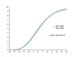
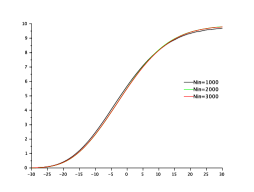
Figure 1. Value function in dimension $2$, for $\rho=0$ on left, and $\rho=0.4$ on right, at $t=0$, and $x_{2}=50$ as a function of $x_{1}-x_{2}$. Here $N_{\mathrm{in}}=1000,2000$, or $3000$, $N_{x}=10$, $N_{w}=1000$.

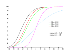
Figure 2. Value function in dimension $2$, for $\rho=0.8$, at $x_{2}=50$ as a function of $x_{1}-x_{2}$ obtained with $N_{x}=10$, $N_{w}=1000$. On left, the value is shown at each time step multiple of $0.05$ and is obtained for $N_{\mathrm{in}}=3000$. On right, the value at time $t=0$ is compared for $N_{\mathrm{in}}=1000$, $2000$ and $3000$ and with the exact solution when $\mathcal{M}$ is a singleton.

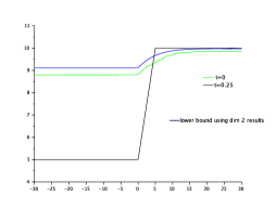
Figure 3. Value function for $\rho=0.8$ in dimension $5$, at $x_{2}=x_{3}=x_{4}=x_{5}=50$ as a function of $x_{1}-x_{2}$. Here $N_{\mathrm{in}}=3000$, $N_{x}=50$, $N_{w}=1000$. On left, the value is shown at each time step multiple of $0.05$. On right, the value at time $t=0$ is compared with a lower bound obtained by using the results in dimension $2$.

References

- [1] Marianne Akian and Eric Fodjo. A probabilistic max-plus numerical method for solving stochastic control problems. In 55th Conference on Decision and Control (CDC 2016), Las Vegas, United States, December 2016. Also arXiv:1605.02816.
- [2] Mohamed Assellaou, Olivier Bokanowski, and Hasnaa Zidani. Error estimates for second order Hamilton-Jacobi-Bellman equations. Approximation of probabilistic reachable sets. Discrete Contin. Dyn. Syst., 35(9):3933–3964, 2015.
- [3] G. Barles and P. E. Souganidis. Convergence of approximation schemes for fully nonlinear second order equations. Asymptotic Anal., 4(3):271–283, 1991.
- [4] J. Frédéric Bonnans and Housnaa Zidani. Consistency of generalized finite difference schemes for the stochastic HJB equation. SIAM J. Numer. Anal., 41(3):1008–1021, 2003.
- [5] Patrick Cheridito, H. Mete Soner, Nizar Touzi, and Nicolas Victoir. Second-order backward stochastic differential equations and fully nonlinear parabolic PDEs. Comm. Pure Appl. Math., 60(7):1081–1110, 2007.
- [6] Arash Fahim, Nizar Touzi, and Xavier Warin. A probabilistic numerical method for fully nonlinear parabolic PDEs. Ann. Appl. Probab., 21(4):1322–1364, 2011.
- [7] Wenjie Guo, Jianfeng Zhang, and Jia Zhuo. A monotone scheme for high-dimensional fully nonlinear PDEs. Ann. Appl. Probab., 25(3):1540–1580, 2015.
- [8] Hidehiro Kaise and William M. McEneaney. Idempotent expansions for continuous-time stochastic control: compact control space. In Proceedings of the 49th IEEE Conference on Decision and Control, Atlanta, Dec. 2010.
- [9] Idris Kharroubi, Nicolas Langrené, and Huyên Pham. A numerical algorithm for fully nonlinear HJB equations: an approach by control randomization. Monte Carlo Methods Appl., 20(2):145–165, 2014.
- [10] Harold J. Kushner. Probability methods for approximations in stochastic control and for elliptic equations. Academic Press [Harcourt Brace Jovanovich, Publishers], New York-London, 1977. Mathematics in Science and Engineering, Vol. 129.
- [11] William M. McEneaney, Hidehiro Kaise, and Seung Hak Han. Idempotent method for continuous-time stochastic control and complexity attenuation. In Proceedings of the 18th IFAC World Congress, 2011, pages 3216–3221, Milano, Italie, 2011.
- [12] J.-M. Mirebeau. Minimal stencils for discretizations of anisotropic PDEs preserving causality or the maximum principle, 2016. Accepted in SIAM Journal on Numerical Analysis (SINUM).