Stokes phenomenon and confluence in non-autonomous Hamiltonian systems

Abstract

This article studies a confluence of a pair of regular singular points to an irregular one in a generic family of time-dependent Hamiltonian systems in dimension 2. This is a general setting for the understanding of the degeneration of the sixth Painlevé equation to the fifth one. The main result is a theorem of sectoral normalization of the family to an integrable formal normal form, through which is explained the relation between the local monodromy operators at the two regular singularities and the non-linear Stokes phenomenon at the irregular singularity of the limit system. The problem of analytic classification is also addressed.

Key words: Non-autonomous Hamiltonian systems  $\cdot$ irregular singularity  $\cdot$ non-linear Stokes phenomenon  $\cdot$ wild monodromy  $\cdot$ confluence  $\cdot$ local analytic classification  $\cdot$ Painlevé equations.

1 Introduction

We consider a parametric family of non-autonomous Hamiltonian systems of the form

$$\begin{aligned} x(x-\epsilon)\tfrac{dy_{1}}{dx}&=\ \tfrac{\partial H}{\partial y_{2}}(y,x,\epsilon)\\ x(x-\epsilon)\tfrac{dy_{2}}{dx}&=-\tfrac{\partial H}{\partial y_{1}}(y,x,\epsilon),\end{aligned}\qquad(y,x,\epsilon)\in(\mathbb{C}^{2}\!\times\!\mathbb{C}\!\times\!\mathbb{C},0),$$ (1)

shortly written as

$$x(x-\epsilon)\tfrac{dy}{dx}=J\mskip 1.0mu\prescript{\smash{\mathrm{t}\mkern-3.0mu}}{}{\mathstrut(D_{y}H)},\qquad J=\left(\begin{smallmatrix}0&1\\[3.0pt] -1&0\end{smallmatrix}\right),$$ (2)

with a singular Hamiltonian function $\frac{H(y,x,\epsilon)}{x(x-\epsilon)}$, where $H(y,x,\epsilon)$ is an analytic germ such that $H(y,0,0)$ has a non-degenerate critical point (Morse point) at $y=0$:

$$D_{y}H(0,0,0)=0,\qquad\det D_{y}^{2}H(0,0,0)\neq 0.$$

The last condition means that the $y$-linear terms of the right side of (2) are of the form

$$A(x,\epsilon)y\ \text{for}\ A=JD_{y}^{2}H,\ \text{where}\ A(0,0)\sim\left(\begin{smallmatrix}\lambda^{(0)}(0)\!\!\!&0\\[3.0pt] 0&\!\!\!-\lambda^{(0)}(0)\end{smallmatrix}\right)\ \text{for some}\ \lambda^{(0)}(0)\neq 0.$$

For $\epsilon\neq 0$ the system (1) has two regular singular points at $x=0$ and $x=\epsilon$. At each one of them, the local information about the system is carried by a formal invariant and a monodromy (holonomy) operator. On the other hand, for $\epsilon=0$ the corresponding information about the irregular singularity at $x=0$ is carried by a formal invariant and by a pair of non-linear operators. Our main goal is to explain the relation between these two distinct phenomena, and to show how the Stokes operators are related to the monodromy operators. The principal thesis is, that while the monodromy operators diverge when $\epsilon\to 0$, they each accumulate to a 1-parameter family of “wild monodromy operators” which encode the Stokes phenomenon (Theorem 34). It is expected that this “wild monodromy” should have Galoisian interpretation.

Along the way, we provide a formal normal form and a sectoral normalization theorem for the family (Theorem 14), an analytic classification (Theorem 31), and a decomposition of the monodromy operators (Theorem 32).

In Section 5, we illustrate all this on the example of traceless $2\times 2$ linear differential systems

$$x(x-\epsilon)\tfrac{dy}{dx}=A(x,\epsilon)y,\qquad A(x,\epsilon)\in\mathfrak{sl}_{2}(\mathbb{C}),\quad\det A(0,0)\neq 0,$$ (3)

for which our description follows from the more general work of Lambert and Rousseau [LR12, HLR13]. Here the relation between the monodromy and the Stokes phenomenon can be summarized as:

Theorem.

When $\epsilon\to 0$ the elements of the monodromy group of the system (3) accumulate to generators of the wild monodromy group of the limit system (that is the group generated by the Stokes operators and the exponential torus).

The linear case can be kept in mind as a leading example of which the general non-linear case is a close analogy.

An important example of a confluent family of systems (1), which in fact motivated this study, is the degeneration of the sixth Painlevé equation to the fifth one, presented in Section 6. A more detailed treatment of this confluence will be the subject of an upcoming article [Kli17].

Acknowledgments

This paper was inspired by the works of C. Rousseau and L. Teyssier [RT08], C. Lambert and C. Rousseau [LR12], and A. Bittmann [Bit16a, Bit16b, Bit16c]. It was written during my stay at Centre de Recherches Mathématiques at Université de Montréal. I want to thank Christiane Rousseau for her support and the CRM for its hospitality.

2 The foliation and its formal invariants

The family of systems (1) defines a family of singular foliations in the $(y,x)$-space, leaves of which are the solutions. We associate to (1) a family of vector fields tangent to the foliations

$$Z_{H,\epsilon}(y,x)=x(x-\epsilon)\partial_{x}+X_{H,x,\epsilon}(y),$$ (4)

where

$$X_{H,x,\epsilon}(y)=\tfrac{\partial H}{\partial y_{2}}(y,x,\epsilon)\partial_{y_{1}}-\tfrac{\partial H}{\partial y_{1}}(y,x,\epsilon)\partial_{y_{2}}.$$ (5)

The vector field $Z_{H,0}(y,x)$ has a saddle-node type singularity at $(y,x)=0$, i.e. its linearization matrix has one zero eigenvalue, corresponding to the $x$-direction. It follows from the Implicit Function Theorem that, for small $\epsilon\neq 0$, $Z_{H,\epsilon}$ has two singular points $(y_{0}(0,\epsilon),0)$ and $(y_{0}(\epsilon,\epsilon),\epsilon)$ bifurcating from $(y_{0}(0,0),0)=0$ and depending analytically on $\epsilon$. The aim of this paper is a study of their confluence when $\epsilon\to 0$.

The two singularities of $Z_{H,\epsilon}$ have each a strong invariant manifold $\mathsf{Y}_{0}=\{(y,x):x=0\}$, resp. $\mathsf{Y}_{\epsilon}=\{(y,x):x=\epsilon\}$. Away of these invariant manifolds the vector field $Z_{H,\epsilon}$ is transverse to the fibration with fibers $\mathsf{Y}_{c}=\{(y,x):x=c\}$. The $(y,x)$-space is endowed with a Poisson structure associated to the 2-form

$$\omega=dy_{1}\wedge dy_{2},$$ (6)

the restriction of which on each fiber $\mathsf{Y}_{c}$ is symplectic. The vector field $Z_{H,\epsilon}$ is transversely Hamiltonian with respect to this fibration, the form $\omega$, and the Hamiltonian function $H(y,x,\epsilon)$.

2.1 Fibered changes of coordinates

We consider the problem of analytic classification of families of systems (1), or orbital analytic classification of vector fields (4), with respect to fiber-preserving (shortly fibered) changes of coordinates

$$(y,x,\epsilon)=(\Phi(u,x,\epsilon),x,\epsilon).$$

Such a change of coordinate transforms a system (2) to a system

$$x(x-\epsilon)\frac{du}{dx} =(D_{u}\Phi)^{-1}J\mskip 1.0mu\prescript{\smash{\mathrm{t}\mkern-3.0mu}}{}{\mathstrut(D_{y}H)}\circ\Phi-x(x-\epsilon)(D_{u}\Phi)^{-1}\tfrac{\partial\Phi}{\partial x}$$

$$=(\det D_{u}\Phi)^{-1}J\mskip 1.0mu\prescript{\smash{\mathrm{t}\mkern-3.0mu}}{}{\mathstrut(D_{u}(H\circ\Phi))}-x(x-\epsilon)(D_{u}\Phi)^{-1}\tfrac{\partial\Phi}{\partial x},$$ (7)

using the identity

$$PJ\mskip 1.0mu\prescript{\smash{\mathrm{t}\mkern-3.0mu}}{}{\mathstrut P}=\det P\cdot J\quad\text{for any $2\!\times\!2$ matrix $P$}.$$ (8)

Definition 1.

We call a fibered transformation $\Phi$ transversely symplectic if $\det(D_{u}\Phi)\equiv 1$, i.e. if it preserves the restriction of $\omega$ to each fiber $\mathsf{Y}_{x}$.

Definition 2.

Two systems (1) with Hamiltonian functions $\frac{H(y,x,\epsilon)}{x(x-\epsilon)}$ and $\frac{\tilde{H}(u,x,\epsilon)}{x(x-\epsilon)}$ are called analytically equivalent if there exists an analytic germ of a transversely symplectic transformation $y=\Phi(u,x,\epsilon)$ that is analytic in $(u,x,\epsilon)$ and transforms one system to another: $\Phi^{*}Z_{H,\epsilon}=Z_{\tilde{H},\epsilon}$.

Lemma 3.

If a transformation $y=\Phi(u,x,\epsilon)$ is transversely symplectic, then the transformed system (7) is transversely Hamiltonian w.r.t. $\omega=du_{1}\wedge du_{2}$.

Proof.

It is enough to show that the system $\frac{du}{dx}=(D_{u}\Phi)^{-1}\tfrac{\partial\Phi}{\partial x}$ is transversely Hamiltonian, that is, denoting $\left(\begin{smallmatrix}f_{1}\\[3.0pt] f_{2}\end{smallmatrix}\right):=(D_{u}\Phi)^{-1}\tfrac{\partial\Phi}{\partial x}$, to show that $\partial{u_{1}}f_{1}+\partial_{u_{2}}f_{2}=0$. Using the identity (8), we can express $f_{1}=\tfrac{1}{\det D_{u}\Phi}\mskip 1.0mu\prescript{\smash{\mathrm{t}\mkern-3.0mu}}{}{\mathstrut(}\partial_{u_{2}}\!\Phi)J\partial_{x}\Phi,\ \ f_{2}=-\tfrac{1}{\det D_{u}\Phi}\mskip 1.0mu\prescript{\smash{\mathrm{t}\mkern-3.0mu}}{}{\mathstrut(}\partial_{u_{1}}\!\Phi)J\partial_{x}\Phi,$ hence

$$\partial_{u_{1}}f_{1}+\partial_{u_{2}}f_{2} =\tfrac{1}{\det D_{u}\Phi}\big{[}\mskip 1.0mu\prescript{\smash{\mathrm{t}\mkern-3.0mu}}{}{\mathstrut(}\partial_{u_{2}}\!\Phi)J\partial_{x}\partial_{u_{1}}\!\Phi-\mskip 1.0mu\prescript{\smash{\mathrm{t}\mkern-3.0mu}}{}{\mathstrut(}\partial_{u_{1}}\!\Phi)J\partial_{x}\partial_{u_{2}}\!\Phi\big{]}$$

$$=\tfrac{1}{\det D_{u}\Phi}\partial_{x}\big{[}\mskip 1.0mu\prescript{\smash{\mathrm{t}\mkern-3.0mu}}{}{\mathstrut(}\partial_{u_{2}}\!\Phi)J\partial_{u_{1}}\!\Phi\big{]}=\tfrac{1}{\det D_{u}\Phi}\partial_{x}\det D_{u}\Phi=0.$$

∎

2.2 The formal invariant $\chi(h,x,\epsilon)$

Theorem 4 (Siegel).

Let $H:(\mathbb{C}^{2},0)\to(\mathbb{C},0)$ have a non-degenerate critical point at $0$, and let $\omega$ be a symplectic volume form. There exists an analytic system of coordinates $u=(u_{1},u_{2})$ in which

$$\omega=du_{1}\wedge du_{2},\qquad\text{and}\qquad H=G_{H}(u_{1}u_{2}).$$

The function $G_{H}$ is uniquely determined by the pair $(H,\omega)$ up to the involution

$$G_{H}(u_{1}u_{2})\mapsto G_{H}(-u_{1}u_{2}),$$ (9)

induced by the symplectic change of variable $J:(u_{1},u_{2})\mapsto(u_{2},-u_{1})$. The pair $(G_{H},\omega)$ is called the Birkhoff-Siegel normal form of the pair $(H,\omega)$. Moreover, if $(H,\omega)$ depend analytically on a parameter, then so does $G_{H}$ and the change of coordinates.

Proof.

While not explicitly stated, the existence part of the theorem is originally proved by Siegel in [SM71, chap. 16 and 17]. See also [Vey77] and [FS94]. The uniqueness can be seen by expressing $G_{H}(h)$ in terms of a period map over a vanishing cycle, see Section 2.2.1 below. ∎

Remark 5.

• The Theorem 4 provides the existence of an analytic transformation of a Hamiltonian vector field $\dot{y}=J\mskip 1.0mu\prescript{\smash{\mathrm{t}\mkern-3.0mu}}{}{\mathstrut(}D_{y}H)$ in dimension 2 to its Birkhoff normal form $\dot{u}=J\mskip 1.0mu\prescript{\smash{\mathrm{t}\mkern-3.0mu}}{}{\mathstrut(}D_{u}G_{H})$, with

  $$G_{H}(h)=\lambda h+\ldots,$$

  where $\pm\lambda\neq 0$ are the eigenvalues of the linear part $JD_{y}^{2}H(0)$. The involution (9) corresponds to the freedom of choice of the eigenvalue $\lambda$.

• The change of coordinates is far from unique. Indeed, the flow of any vector field $\xi=a(u_{1}u_{2})\big{(}u_{1}\partial_{u_{1}}-u_{2}\partial_{u_{2}}\big{)}$ preserves the normal form.

Let $H=H(y,x,\epsilon)$ be our germ. By the implicit function theorem, for each small $(x,\epsilon)$, the function $H(\cdot,x,\epsilon)$ has an isolated non-degenerate critical point $y_{0}(x,\epsilon)$, depending analytically on $(x,\epsilon)$. Let $y=\Phi(u,x,\epsilon)$ be the transformation to the Birkhoff-Siegel normal form for the function $y\mapsto H(y,x,\epsilon)$ and the form $\omega=dy_{1}\wedge dy_{2}$, depending analytically on $(x,\epsilon)$, i.e.

$$H(\cdot,x,\epsilon)\circ\Phi(u,x,\epsilon)=G_{H}(u_{1}u_{2},x,\epsilon),\qquad\det D_{u}\Phi(u,x,\epsilon)\equiv 1.$$

By (7), it brings the system (1) to a prenormal form

$$x(x-\epsilon)\frac{du}{dx} =J\mskip 1.0mu\prescript{\smash{\mathrm{t}\mkern-3.0mu}}{}{\mathstrut(D_{u}G_{H})}+O(x(x-\epsilon))$$

$$=\chi(u_{1}u_{2},x,\epsilon)\left(\begin{smallmatrix}1&0\\[3.0pt] 0&-1\end{smallmatrix}\right)u+O(x(x-\epsilon)),$$ (10)

where

$$\chi(h,x,\epsilon)=\chi^{(0)}(h,\epsilon)+x\chi^{(1)}(h,\epsilon):=\tfrac{\partial G_{H}}{\partial h}(h,x,\epsilon)\mod x(x-\epsilon),$$ (11)

$h=u_{1}u_{2}$, or equivalently,

$$\chi(h,x,\epsilon)=\left\{\!\!\begin{array}[]{l}\tfrac{1}{\epsilon}\big{[}x\tfrac{\partial G_{H}}{\partial h}(h,\epsilon,\epsilon)-(x-\epsilon)\tfrac{\partial G_{H}}{\partial h}(h,0,\epsilon)\big{]},\quad\epsilon\neq 0,\\[6.0pt] \tfrac{\partial G_{H}}{\partial h}(h,0,0)+x\tfrac{\partial^{2}G_{H}}{\partial h\partial x}(h,0,0),\quad\epsilon=0.\end{array}\right.$$ (12)

Definition 6.

The function $\chi(h,x,\epsilon)$ is called a formal invariant of the system (1).

For $\epsilon\neq 0$ the formal invariant $\chi$ is completely determined by the functions $G_{H}(\cdot,0,\epsilon)$ and $G_{H}(\cdot,\epsilon,\epsilon)$ , which are analytic invariants of the autonomous Hamiltonian systems $X_{H,0,\epsilon}$, $X_{H,\epsilon,\epsilon}$ (5) on the strong invariant manifolds $\mathsf{Y}_{0},\mathsf{Y}_{\epsilon}$.

Corollary 7.

The formal invariant $\chi(h,x,\epsilon)$ is well-defined up to the involution

$$J^{*}:\chi(h,x,\epsilon)\mapsto-\chi(-h,x,\epsilon),$$ (13)

induced by the symplectic transformation $u\mapsto Ju$. It is uniquely determined by the polar part of the Hamiltonian $\frac{H(y,x,\epsilon)}{x(x-\epsilon)}$, and it is invariant with respect to fibered transversely symplectic changes of coordinates.

Let

$$\lambda(x,\epsilon)=\chi(0,x,\epsilon).$$

Then $\pm\lambda(x,\epsilon)$ are the eigenvalues of the matrix $A(x,\epsilon)=J\mskip 1.0mu\prescript{\smash{\mathrm{t}\mkern-3.0mu}}{}{\mathstrut D_{y}^{2}H(0,x,\epsilon)}$ modulo $x(x-\epsilon)$, see Example 8, and the involution (13) corresponds to the freedom of choice of the eigenvalue $\lambda$.

Example 8 (Traceless linear systems).

A traceless linear system

$$x(x-\epsilon)\frac{dy}{dx}=A(x,\epsilon)y,$$ (14)

with $\mathrm{tr}A(x,\epsilon)=0$ and $A(0,0)\sim\left(\begin{smallmatrix}\lambda^{(0)}(0)&0\\[3.0pt] 0&-\lambda^{(0)}(0)\end{smallmatrix}\right)$ for some $\lambda^{(0)}(0)\neq 0$, is of the form (2) for the quadratic form $H(y,x,\epsilon)=\tfrac{1}{2}\mskip 1.0mu\prescript{\smash{\mathrm{t}\mkern-3.0mu}}{}{\mathstrut y}J\mskip 1.0mu\prescript{\smash{\mathrm{t}\mkern-3.0mu}}{}{\mathstrut A(x,\epsilon)}y$. Let $\pm\tilde{\lambda}(x,\epsilon)$ be the eigenvalues of $A(x,\epsilon)$, and let $C(x,\epsilon)$ be a corresponding matrix of eigenvectors of $A(x,\epsilon)$, depending analytically on $(x,\epsilon)$ and normalized so that $\det C(x,\epsilon)=1$. The change of variable $y=C(x,\epsilon)u$, brings the system (14) to

$$x(x-\epsilon)\frac{du}{dx}=\tilde{\lambda}(x,\epsilon)\left(\begin{smallmatrix}1&0\\ 0&-1\end{smallmatrix}\right)u+x(x-\epsilon)C^{-1}\frac{dC}{dx}.$$

Denoting $\lambda(x,\epsilon):=\big{(}\lambda^{(0)}(\epsilon)+x\lambda^{(1)}(\epsilon)\big{)}=\tilde{\lambda}(x,\epsilon)\mod x(x-\epsilon)$, then we have $\chi(h,x,\epsilon)=\pm\lambda(x,\epsilon)$.

2.2.1 Geometric interpretation of the invariant $\chi$.

For each small $(x,\epsilon)$, the function $H(\cdot,x,\epsilon)$ has an isolated non-degenerate critical point $y_{0}(x,\epsilon)$, depending analytically on $(x,\epsilon)$, with a critical value $h_{0}(x,\epsilon)$. For $(x,\epsilon)$ fixed, $h\in(\mathbb{C},h_{0})$, consider the germ of the level set $S_{h}(x,\epsilon)=\{y\in(\mathbb{C}^{2},y_{0}(x,\epsilon)):H(y,x,\epsilon)=h\}\subset\mathsf{Y}_{x}$. As a basic fact of the Picard–Lefschetz theory [AVG12], we know that if $h$ is a non-critical value for $H(\cdot,x,\epsilon)$, i.e. $h\neq h_{0}$, then $S_{h}(x,\epsilon)$ has the homotopy type of a circle. Let $\gamma_{h}(x,\epsilon)$ depending continuously on $(x,\epsilon)$ be a loop generating the first homology group of $S_{h}(x,\epsilon)$, the so called vanishing cycle. And let $\mu$ be a 1-form such that $\omega=dH\wedge\mu;$ its restriction to a non-critical level $S_{h}(x,\epsilon)$ is called the Gelfand-Leray form of $\omega$ and is denoted

$$\mu=\frac{\omega}{dH}.$$

Its period function over the vanishing cycle

$$p(h,x,\epsilon):=\tfrac{1}{2\pi i}\int_{\gamma_{h}(x,\epsilon)}\frac{\omega}{dH},$$ (15)

is well-defined up to a sign change (orientation of $\gamma_{h}$), and depends analytically on $(x,\epsilon)$ [AVG12, chap. 10]. Let $G_{H}(\cdot,x,\epsilon)$ be the inverse of the function $h\mapsto\int_{h_{0}(x,\epsilon)}^{h}p(s,x,\epsilon)\,ds$. Then $(G_{H},\omega)$ is the Birkhoff-Siegel normal form of $(H,\omega)$.

Indeed, the above formula for $G_{H}$ is invariant with respect to analytic transversely symplectic changes of coordinates: Supposing that $H=g(y_{1}y_{2},x,\epsilon)$ is in its Birkhoff-Siegel normal form, then the level sets are written as $S_{h}=\{y_{1}\neq 0,\ y_{2}=\tfrac{g^{\circ(-1)}(h,x,\epsilon)}{y_{1}}\}$, and $\frac{\omega}{dH}=\frac{dy_{1}}{y_{1}\cdot\frac{\partial g}{\partial(y_{1}y_{2})}\circ g^{\circ(-1)}(h,x,\epsilon)}$, and therefore $p(h)=\big{(}\frac{\partial g}{\partial(y_{1}y_{2})}\big{)}^{-1}\circ g^{\circ(-1)}(h,x,\epsilon)$, i.e. $G_{H}=g$.

The above formula for the the Birkhoff-Siegel normal form and hence for the formal invariant $\chi$ involves a double inversion which makes it difficult to calculate. The following proposition, which will be proved in Section 7.4, allows to determine it in some special cases. This will be useful in the case of the fifth Painlevé equation (Section 6).

Proposition 9 (Birkhoff-Siegel normal form of an autonomous Hamiltonian system).

Let $H(y)$ be of the form

$$H(y)=G(h)+y_{i}\Delta(y_{i},h),\quad h=y_{1}y_{2},$$

for some $i\in\{1,2\}$, with $G,\Delta$ analytic germs, and

$$G(h)=\lambda h+O(h^{2}),\quad\lambda\neq 0.$$

Then $(G,\omega)$ is the Birkhoff-Siegel normal form for the pair $(H,\omega)$, $\omega=dy_{1}\wedge dy_{2}$.

Corollary 10 (Invariant $\chi$ for $\epsilon=0$).

For $\epsilon=0$, suppose that

$$H(y,x,0)=G^{(0)}(h,0)+xH^{(1)}(y,0)+O(x^{2}),\quad h=y_{1}y_{2},$$

where $G^{(0)}(h,0)=\lambda^{(0)}(0)h+O(h^{2})$, $\lambda^{(0)}(0)\neq 0$. Write

$$H^{(1)}(y,0)=G^{(1)}(h,0)+y_{1}\Delta_{1}(y_{1},h,0)+y_{2}\Delta_{2}(y_{2},h,0),$$

with $\Delta_{i}(y_{i},h,0)=O(y_{i})$. Then

$$\chi(h,x,0)=\tfrac{\partial}{\partial h}\big{(}G^{(0)}(h,0)+x\,G^{(1)}(h,0)\big{)}$$

is the formal invariant of the vector field $Z_{H,0}=x^{2}\partial_{x}+X_{H}$ associated to $H$.

Proof.

Consider a deformation

$$H(y,x,\epsilon)=G^{(0)}(h,0)+xG^{(1)}(h,0)+xy_{1}\Delta_{1}(y_{1},h,0)+(x-\epsilon)y_{2}\Delta_{2}(y_{2},h,0)+O(x(x-\epsilon)),$$

and calculate the Birkhoff-Siegel invariants for $H(y,0,\epsilon)$, $H(y,\epsilon,\epsilon)$, using Proposition 9. ∎

2.3 Model system (formal normal form)

Definition 11 (Model family).

Let $\chi(h,x,\epsilon)$ be the formal invariant of the system (1). The model family (formal normal form) for the the system (1) is the family of systems

$$x(x-\epsilon)\tfrac{du_{1}}{dx} =\ \chi(u_{1}u_{2},x,\epsilon)\cdot u_{1}$$ (16)

$$x(x-\epsilon)\tfrac{du_{2}}{dx} =-\chi(u_{1}u_{2},x,\epsilon)\cdot u_{2},$$

which is Hamiltonian with respect to the Hamiltonian function $\frac{G(u_{1}u_{2},x,\epsilon)}{x(x-\epsilon)}$,

$$G(h,x,\epsilon)=\int_{0}^{h}\chi(s,x,\epsilon)\,ds.$$ (17)

The formal normal form of the family $Z_{H,\epsilon}$ is the associated family of vector fields

$$Z_{G,\epsilon}=x(x-\epsilon)\partial_{x}+\chi(u_{1}u_{2},x,\epsilon)\big{(}u_{1}\partial_{u_{1}}-u_{2}\partial_{u_{2}}\big{)}.$$ (18)

The system (16) is integrable with the function $h(u)=u_{1}u_{2}$ being its first integral, $Z_{G,\epsilon}\cdot h=0$. The general solutions of (16) are of the form

$$\begin{aligned} u_{1}(x,\epsilon;c)&=c_{1}E_{\chi}(c_{1}c_{2},x,\epsilon),\\ u_{2}(x,\epsilon;c)&=c_{2}E_{\chi}(c_{1}c_{2},x,\epsilon)^{-1},\end{aligned}\qquad c=(c_{1},c_{2})\in\mathbb{C}^{2},$$ (19)

where

$$E_{\chi}(h,x,\epsilon)=\left\{\!\!\begin{array}[]{ll}x^{-\frac{\chi^{(0)}(h,\epsilon)}{\epsilon}}(x-\epsilon)^{\frac{\chi^{(0)}(h,\epsilon)}{\epsilon}+\chi^{(1)}(h,\epsilon)},&\text{for $\epsilon\neq 0$},\\[6.0pt] e^{-\frac{\chi^{(0)}(h,0)}{x}}x^{\chi^{(1)}(h,0)},&\text{for $\epsilon=0$}.\end{array}\right.$$ (20)

3 Formal and sectoral normalization theorem

Throughout the text we will denote

$$\mathsf{Y}=\{|y|<\delta_{y}\},\qquad\mathsf{U}=\{|u|<\delta_{u}\},\qquad\mathsf{X}=\{|x|<\delta_{x}\},\qquad\mathsf{E}=\{|\epsilon|<\delta_{\epsilon}\},$$ (21)

for some $\delta_{y},\delta_{u},\delta_{x},\delta_{\epsilon}>0$, and implicitly suppose that $\delta_{\epsilon}<<\delta_{x}$ so that the singular points $x=0,\epsilon$ are both well inside $\mathsf{X}$.

Definition 12 (Family of spiraling sectoral domains $\mathsf{X}_{\pm}(\epsilon)$, $\epsilon\in\mathsf{E}_{\pm}$).

Let $\eta>0$ be an arbitrarily small constant, and let $\delta_{x}>>\delta_{\epsilon}>0$ be radii of small discs at 0 in the $x$-and $\epsilon$-space. Let $\lambda(x,\epsilon)=\chi(0,x,\epsilon),$ and let

$$\mathsf{E}_{\pm}:=\{|\epsilon|<\delta_{\epsilon},\ |\arg\big{(}\pm\tfrac{\epsilon}{\lambda(0,0)}\big{)}|<\pi-2\eta\},$$ (22)

be two sectors in the $\epsilon$-space. For $\epsilon\in\mathsf{E}_{\pm}$ define a domain

$$\mathsf{X}_{\pm}(\epsilon)$$

in the $x$-space as a simply connected ramified domain spanned by the complete real trajectories of the vector fields

$$e^{i\omega_{\pm}}\cdot\tfrac{x(x-\epsilon)}{\lambda(x,\epsilon)}\partial_{x}$$ (23)

that never leave the disc of radius $\delta_{x}$, where the phase $\omega_{\pm}$ varies continuously in the interval

$$\left\{\!\!\begin{array}[]{l}\max\{0,\arg(\frac{\pm\epsilon}{\lambda(0,0)})\}-\frac{\pi}{2}+\eta<\omega_{\pm}<\min\{0,\arg(\frac{\pm\epsilon}{\lambda(0,0)})\}+\frac{\pi}{2}-\eta,\quad\text{for $\epsilon\neq 0$},\\[6.0pt] |\omega_{\pm}|<\frac{\pi}{2}-\eta,\quad\text{for $\epsilon=0$.}\end{array}\right.$$ (24)

The constraints (24) on the variation of $\omega_{\pm}$ are such that the real dynamics of the vector field (23) and the asymptotic behavior of the solutions (19) would not change drastically depending on $\omega_{\pm}$. Namely, for $\epsilon\neq 0$:

• The point $x=\epsilon$ is repulsive when $|\arg\frac{\epsilon}{\lambda(x,\epsilon)}-\omega_{\pm}|<\frac{\pi}{2}$ and attractive when $|\arg\frac{-\epsilon}{\lambda(x,\epsilon)}-\omega_{\pm}|<\frac{\pi}{2}$, and vice-versa for the point $x=0$.

• The $u_{1}$-component of the solution (19) tends to $0$ along a negative real trajectory of (23) and to $\infty$ along a positive real trajectory for $|\omega_{\pm}|<\tfrac{\pi}{2}$, and vice-versa for the $u_{2}$-component.

For $\epsilon=0$, the domain $\mathsf{X}_{+}(0)=\mathsf{X}_{-}(0)$ consists of a pair of overlapping sectoral domains $\mathsf{X}^{\scalebox{0.7}{\!$\mathrlap{\rotatebox[origin={c}]{-45.0}{$\LEFTCIRCLE$}}\rotatebox[origin={c}]{-135.0}{$\LEFTCIRCLE$}\!$}}(0),\mathsf{X}^{\scalebox{0.7}{\!$\mathrlap{\rotatebox[origin={c}]{45.0}{$\LEFTCIRCLE$}}\rotatebox[origin={c}]{135.0}{$\LEFTCIRCLE$}\!$}}(0)$ of opening $2\pi-2\eta$ with a common point at $x=0$. See Figure 1.

Denoting $x_{1,\pm}(\epsilon)$ the attractive equilibrium point of (23) and $x_{2,\pm}(\epsilon)$ the repulsive one,

$$x_{1,+}(\epsilon)=x_{2,-}(\epsilon)=0,\qquad x_{1,-}(\epsilon)=x_{2,+}(\epsilon)=\epsilon,$$ (25)

then

$$u_{i}(x,\epsilon)\to\infty,\ u_{j}(x,\epsilon)\to 0,\ (j=3-i),\ \text{ when }\ x\to x_{i,\pm}(\epsilon)\ \text{along a real trajectory of \eqref{eq:HC-xvectfield}}.$$

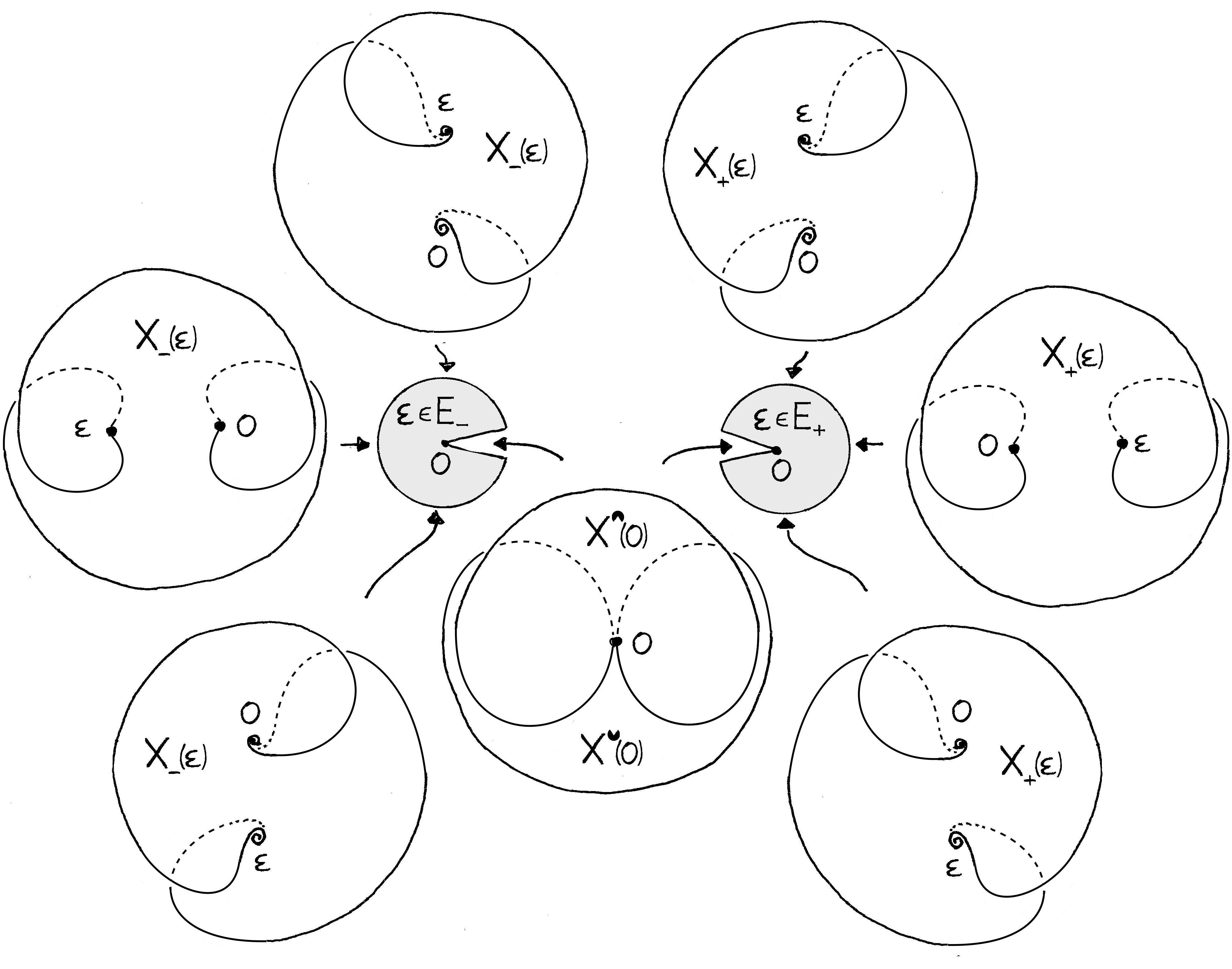
Figure 1: The domains $\mathsf{X}_{\pm}(\epsilon)$ in dependence on $\epsilon\in\mathsf{E}_{\pm}$. (Picture with $\lambda^{(0)}(0)=1$.)

Before giving a general theorem on sectoral normalization for the parametric family (1), let us first state it for the limit system with $\epsilon=0$ which has an irregular singularity of Poincaré rank 1 at $x=0$.

Theorem 13 (Formal and sectoral normalization at $\epsilon=0$).

The system (1) with $\epsilon=0$ can be brought to its formal normal form (16) through a formal transversely symplectic change of coordinates

$$(y,x)=(\hat{\mathbf{\Psi}}(u,x,0),x),\qquad\hat{\mathbf{\Psi}}(u,x,0)=\sum_{k\geq 0}\psi^{(k)}(u)x^{k},$$ (26)

where $\psi^{(k)}(u)$ are analytic in $u$ on a fixed neighborhood $\mathsf{U}$ of $0$. This formal series is generally divergent, but it is Borel 1-summable, with a pair of Borel sums $\mathbf{\Psi}^{\scalebox{0.7}{\!$\mathrlap{\rotatebox[origin={c}]{-45.0}{$\LEFTCIRCLE$}}\rotatebox[origin={c}]{-135.0}{$\LEFTCIRCLE$}\!$}}(u,x,0)$ and $\mathbf{\Psi}^{\scalebox{0.7}{\!$\mathrlap{\rotatebox[origin={c}]{45.0}{$\LEFTCIRCLE$}}\rotatebox[origin={c}]{135.0}{$\LEFTCIRCLE$}\!$}}(u,x,0)$ defined respectively above the sectors $x\in\mathsf{X}^{\scalebox{0.7}{\!$\mathrlap{\rotatebox[origin={c}]{-45.0}{$\LEFTCIRCLE$}}\rotatebox[origin={c}]{-135.0}{$\LEFTCIRCLE$}\!$}}(0),\mathsf{X}^{\scalebox{0.7}{\!$\mathrlap{\rotatebox[origin={c}]{45.0}{$\LEFTCIRCLE$}}\rotatebox[origin={c}]{135.0}{$\LEFTCIRCLE$}\!$}}(0)$ of Definition 12 (for some $0<\eta<\tfrac{\pi}{2}$ arbitrarily small and some $\delta_{x}>0$ depending on $\eta$), and $u\in\mathsf{U}$. The fibered sectoral transformations $(y,x)=(\mathbf{\Psi}^{\bullet}(u,x,0)$, $\bullet=\scalebox{0.7}{\!$\mathrlap{\rotatebox[origin={c}]{-45.0}{$\LEFTCIRCLE$}}\rotatebox[origin={c}]{-135.0}{$\LEFTCIRCLE$}\!$},\scalebox{0.7}{\!$\mathrlap{\rotatebox[origin={c}]{45.0}{$\LEFTCIRCLE$}}\rotatebox[origin={c}]{135.0}{$\LEFTCIRCLE$}\!$}$, are transversely symplectic and bring the system (1) with $\epsilon=0$ to its formal normal form.

The Theorem 13 is originally due to Takano [Tak90] for systems (1) whose formal invariant is of the form $\chi(h,x)=\lambda^{(0)}+x\chi^{(1)}(h)$. In the case of the irregular singularity of the fifth Painlevé equation it was proved earlier by Takano [Tak83]. Some similar and closely related theorems are due to Shimomura [Shi83], Yoshida [Yos84], and recently by Bittmann [Bit16a, Bit16b], which apply to doubly resonant systems $x^{2}\frac{dy}{dx}=F(y,x)$, with $D_{y}F(0,0)=\lambda^{(0)}(0)\left(\begin{smallmatrix}1&\\ &-1\end{smallmatrix}\right)$ under a condition on positivity of $\mathrm{tr}\frac{\partial}{\partial x}D_{y}F(0,0)$. This condition is not satisfied for Hamiltonian systems (1) but nevertheless allows to treat Painlevé equations.

Theorem 14 (Formal and sectoral normalization).

Let $Z_{H,\epsilon}(y,x)$ be a family of vector fields (4) and let $\chi(h,x,\epsilon)$ be their formal invariant.

(i) There exists a formal transversely sympectic change of coordinates $(y,x,\epsilon)=(\hat{\mathbf{\Psi}}(u,x,\epsilon),x,\epsilon)$ written as a formal power series

$$\hat{\mathbf{\Psi}}(u,x,\epsilon)=\psi^{(0)}(u,\epsilon)+x\psi^{(1)}(u,\epsilon)+x(x-\epsilon)\sum_{k,l\geq 0}\tilde{\psi}^{(kl)}(u)x^{k}\epsilon^{l},$$ (27)

with $\psi^{(0)}(u,\epsilon)$, $\psi^{(1)}(u,\epsilon)$ analytic in $(u,\epsilon)$, and $\tilde{\psi}^{(kl)}(u)$ analytic in $u$ on a fixed neighborhood $\mathsf{U}=\{|u_{1}|,|u_{2}|<\delta_{u}\}$ of $0$, which brings $Z_{\epsilon}$ to its formal normal form (18). The coefficients $\tilde{\psi}^{(kl)}$ grow at most factorially in $k+l$:

$$\max_{u\in\mathsf{U}}\|\tilde{\psi}^{(kl)}(u)\|\leq L^{k+l}(k+l)!\quad\text{for some}\quad L>0.$$

(ii) There exists a transversely symplectic fibered change of coordinates $(y,x,\epsilon)=(\mathbf{\Psi}_{\pm}(u,x,\epsilon),x,\epsilon)$, with $\mathbf{\Psi}_{\pm}(u,0,\epsilon)=\psi^{(0)}(u,\epsilon)$ (27), defined for $x$ in the spiraling domain $\mathsf{X}_{\pm}(\epsilon)$, $\epsilon\in\mathsf{E}_{\pm}$, of Definition 12 (for some $0<\eta<\tfrac{\pi}{2}$ arbitrarily small and some $\delta_{x},\delta_{\epsilon}>0$ depending on $\eta$), and for $u\in\mathsf{U}$, which brings $Z_{\epsilon}$ to its formal normal form (18). It is uniformly continuous on

$$\mathsf{XE}_{\pm}=\{(x,\epsilon)\mid x\in\mathsf{X}_{\pm}(\epsilon)\}$$

and analytic on its interior. When $\epsilon$ tends radially to $0$ with $\arg\epsilon=\beta$, then $\mathbf{\Psi}_{\pm}(u,x,\epsilon)$ converges to $\mathbf{\Psi}_{\pm}(u,x,0)$ uniformly on compact sets of the sub-domains $\lim_{\begin{subarray}{c}\epsilon\to 0\\ \arg\epsilon=\beta\end{subarray}}\mathsf{X}_{\pm}(\epsilon)\subseteq\mathsf{X}(0)$. Note that in our notation $\mathbf{\Psi}_{\pm}(u,x,0)$ consists of a pair of sectoral transformations $\mathbf{\Psi}^{\scalebox{0.7}{\!$\mathrlap{\rotatebox[origin={c}]{-45.0}{$\LEFTCIRCLE$}}\rotatebox[origin={c}]{-135.0}{$\LEFTCIRCLE$}\!$}}(u,x,0)$ and $\mathbf{\Psi}^{\scalebox{0.7}{\!$\mathrlap{\rotatebox[origin={c}]{45.0}{$\LEFTCIRCLE$}}\rotatebox[origin={c}]{135.0}{$\LEFTCIRCLE$}\!$}}(u,x,0)$; it is a functional cochain using the terminology of [IY08].

(iii) Let $\tilde{\Psi}(u,x,\epsilon)$ be an analytic extension of the function given by the convergent series

$$\tilde{\Psi}(u,x,\epsilon)=\sum_{k,l\geq 0}\frac{\tilde{\psi}^{(kl)}(u)}{(k+l)!}x^{k}\epsilon^{l},\quad\text{$\tilde{\psi}^{(kl)}$ as in \eqref{eq:HC-hatPhi}}.$$

For each point $(x,\epsilon)$, for which there is $\theta\in\,]\!-\!\frac{\pi}{2},\frac{\pi}{2}[$ such that $\mbox{$\mathbf{S}_{\theta}\cdot(x,\epsilon)$}\subseteq\mathsf{XE}_{\pm}$, with $\mathbf{S}_{\theta}\subset\mathbb{C}$ denoting the circle through the points $0$ and $1$ with center on $e^{i\theta}\mathbb{R}^{+}$, we can express $\mathbf{\Psi}_{\pm}(u,x,\epsilon)$ through the following Laplace transform of $\tilde{\Psi}$:

$$\mathbf{\Psi}_{\pm}(u,x,\epsilon)=\psi^{(0)}(u,\epsilon)+x\psi^{(1)}(u,\epsilon)+x(x-\epsilon)\int_{0}^{+\infty e^{i\theta}}\!\!\!\tilde{\Psi}(u,sx,s\epsilon)\,e^{-s}\,ds.$$ (28)

In particular, $\mathbf{\Psi}_{\pm}(u,x,0)$ is the pair of sectoral Borel sums $\mathbf{\Psi}^{\scalebox{0.7}{\!$\mathrlap{\rotatebox[origin={c}]{-45.0}{$\LEFTCIRCLE$}}\rotatebox[origin={c}]{-135.0}{$\LEFTCIRCLE$}\!$}}(u,x,0)$, $\mathbf{\Psi}^{\scalebox{0.7}{\!$\mathrlap{\rotatebox[origin={c}]{45.0}{$\LEFTCIRCLE$}}\rotatebox[origin={c}]{135.0}{$\LEFTCIRCLE$}\!$}}(u,x,0)$ of the formal series $\hat{\mathbf{\Psi}}(u,x,0)$.

As a consequence, $\mathbf{\Psi}_{\pm}$ and $\hat{\mathbf{\Psi}}$ satisfy the same $(\partial_{u},\partial_{x},\partial_{\epsilon})$-differential relations with meromorphic coefficients.

The proof will be given in Section 7.

The transformations $\mathbf{\Psi}_{\pm}$ and $\hat{\mathbf{\Psi}}$ are unique up to left composition with an analytic symmetry of the model system, see Corollary 27.

Corollary 15.

The system (1) possesses:

• a formal first integral given by $h\circ\hat{\mathbf{\Psi}}^{\circ(-1)}(y,x,\epsilon)$, where $\hat{\mathbf{\Psi}}$ as above and $h(u)=u_{1}u_{2}$ is a first integral of the model system,

• an actual first integral given by $h\circ\mathbf{\Psi}_{\pm}^{\circ(-1)}(y,x,\epsilon)$ that is bounded and analytic on the domain $\mathsf{XE}_{\pm}$.

Definition 16.

The solution $y=\mathbf{\Psi}_{\pm}(0,x,\epsilon)$ is called ramified center manifold. It is the unique solution that is bounded on $\mathsf{X}_{\pm}(\epsilon)$ (cf. [Kli16]).

Remark 17.

In the variable $x=\epsilon z$, the system (2) takes the form of a singularly perturbed system

$$\epsilon z(z-1)\tfrac{dy}{dz}=J\mskip 1.0mu\prescript{\smash{\mathrm{t}\mkern-3.0mu}}{}{\mathstrut(D_{y}H)(y,\epsilon z,\epsilon)}.$$

The domains $z\in\frac{1}{\epsilon}\mathsf{X}_{\pm}(\epsilon)$, $\epsilon\in\mathsf{E}_{\pm}$, then correspond to the Stokes domains in the sense of exact WKB analysis [KT05], where the Stokes curves would be the real separatrices of the point $z=\infty$ of the vector field (23) $e^{i(\omega_{\pm}+\arg\epsilon)}\frac{z(z-1)}{\lambda(0,0)}\partial_{z}$ with a fixed phase $\omega_{\pm}$ (24).

4 Stokes operators and accumulation of monodromy

We will define several operators acting as transversely symplectic fibered isotropies on the three following foliations given by three different vector fields:

• Foliation in the $(u,x)$-space given by the model vector field $Z_{G,\epsilon}$ (18).

• Foliation in the $(c,x)$-space, $c$ being the constant of initial condition in (19), given by the rectified vector field $Z_{0,\epsilon}=x(x-\epsilon)\partial_{x}$. Note that a fibered isotropy of $Z_{0,\epsilon}$ is necessarily independent of $x$; it acts on the $c$-space of initial conditions only.

• Foliation in the $(y,x)$-space given by the original vector field $Z_{H,\epsilon}$ (4).

4.1 Symmetries of the model system: exponential torus

A vertical infinitesimal symplectic symmetry (shortly infinitesimal symmetry) of the normal form vector field $Z_{G,\epsilon}$ (18) is a germ of vector field $\xi$ in the $(u,x)$-space that preserves:

• the $x$-coordinate: $\mathcal{L}_{\xi}x=\xi\cdot x=0$,

• the symplectic form $\omega=du_{1}\wedge du_{2}$:  $\mathcal{L}_{\xi}\omega=0$,

• the vector field $Z_{G,\epsilon}$:  $\mathcal{L}_{\xi}Z_{G,\epsilon}=[\xi,Z_{G,\epsilon}]=0.$

Lemma 18.

A vector field $\xi$ is an infinitesimal symmetry of $Z_{G,\epsilon}$ if and only if $\xi=X_{f,x,\epsilon}$ is a Hamiltonian vector field with respect to $\omega$ for a first integral $f(u,x,\epsilon)$ of $Z_{G,\epsilon}$:

$$Z_{G,\epsilon}\cdot f=0.$$

Proof.

The conditions (i) and (ii) say that $\xi=a_{1}(u,x,\epsilon)\partial_{u_{1}}+a_{2}(u,x,\epsilon)\partial_{u_{2}}$ with $\frac{\partial a_{1}}{\partial u_{1}}+\frac{\partial a_{2}}{\partial u_{2}}=0$, i.e. $a_{1}=\frac{\partial f}{\partial u_{2}}$, $a_{2}=-\frac{\partial f}{\partial u_{1}}$ for some $f$, and $\xi=\frac{\partial f}{\partial u_{2}}\partial_{u_{1}}-\frac{\partial f}{\partial u_{1}}\partial_{u_{2}}=X_{f}$.

The condition (iii) says that

$$0=Z_{G,\epsilon}\cdot D_{u}f-X_{f,x,\epsilon}\cdot D_{u}G=D_{u}(Z_{G,\epsilon}\cdot f).$$

Up to a translation $f(u,x,\epsilon)\mapsto f(u,x,\epsilon)-f(0,x,\epsilon)$ which does not affect $X_{f,x,\epsilon}$, this condition is equivalent to $Z_{G,\epsilon}\cdot f=0$. ∎

The vector field $Z_{G,\epsilon}$ has the following obvious first integrals (cf. (19)):

$$c_{1}(u,x,\epsilon)=u_{1}\cdot E_{\chi}(h,x,\epsilon)^{-1},\qquad c_{2}(u,x,\epsilon)=u_{2}\cdot E_{\chi}(h,x,\epsilon),$$ (29)

and

$$h(u)=u_{1}u_{2}=c_{1}c_{2},$$

where $E_{\chi}(h,x,\epsilon)$ is as in (20). Clearly, any function of $c=(c_{1},c_{2})$ is again a first integral, and since $c$ defines local coordinates on the space of leaves (space of initial conditions), the converse is also true. Note that the map $c:u\mapsto c(u,x,\epsilon)$ conjugates the vector field $Z_{G,\epsilon}$ to the “rectified” vector field $Z_{0,\epsilon}=x(x-\epsilon)\partial_{x}$ in the $(c,x)$-space:

$$Z_{G,\epsilon}=c^{*}(x(x-\epsilon)\partial_{x}).$$

It turns out that analytic first integrals are functions of $h=c_{1}c_{2}$ only.

Proposition 19.

If $f(u,x,\epsilon)$ is an analytic (resp. meromorphic) first integral of $Z_{G,\epsilon}$ on some neighborhood $\mathsf{U}\times\mathsf{X}\times\mathsf{E}$ of 0, then $f=F(u_{1}u_{2},\epsilon)$ with $F$ analytic (resp. meromorphic).

Proof of Proposition 19.

On one hand, $c_{1}(u,x,\epsilon)$, $c_{2}(u,x,\epsilon)$ are local coordinate on the space of leaves, hence any first integral is a function of them (depending on $\epsilon$). On the other hand, any analytic germ $f(u,x,\epsilon)$ is uniquely decomposed as $f=f_{0}(h,x,\epsilon)+u_{1}f_{1}(u_{1},h,x,\epsilon)+u_{2}f_{2}(u_{2},h,x,\epsilon)$, with $f_{l}$ analytic. Writing $u_{i}=c_{i}(u,x,\epsilon)\cdot E_{\chi}^{-(-1)^{i}}(h,x,\epsilon)$ (20), we see that for $f$ to be bounded when $x\to x_{i,\pm}$, we must have $f_{i}=0$, $i=1,2$. Therefore $f=f_{0}$ which must then be independent of $x$.

A meromorphic function is a quotient of analytic ones. ∎

Remark 20.

The statement remains true also if restricted to $\epsilon=0$, or a generic fixed $\epsilon$ (such that $\tfrac{\lambda^{(0)}(\epsilon)}{\epsilon}\notin\mathbb{Z}$).

Corollary 21.

The Lie algebra of analytic infinitesimal symmetries of $Z_{G,\epsilon}$ consists of Hamiltonian vector fields

$$\xi=a(u_{1}u_{2},\epsilon)\big{(}u_{1}\partial_{u_{1}}-u_{2}\partial_{u_{2}}\big{)}=a(h,\epsilon)X_{h},\qquad\textit{$a(h,\epsilon)$ analytic},$$ (30)

and is commutative. It is also called the infinitesimal torus.

The time-$1$ flow map of a vector field (30) is given by

$$u\mapsto\mathcal{T}_{a}(u):=\Phi^{1}_{aX_{h}}(u)=\left(\begin{smallmatrix}e^{a(h,\epsilon)}&0\\[3.0pt] 0&e^{-a(h,\epsilon)}\end{smallmatrix}\right)u.$$ (31)

Definition 22.

A (transversely symplectic fibered) isotropy of the model vector field $Z_{G,\epsilon}$ is a germ of symplectic transformation $(u,x,\epsilon)\mapsto(\phi(u,x,\epsilon),x,\epsilon)$ analytic in $u\in\mathsf{U}$, such that $\phi^{*}Z_{G,\epsilon}=Z_{G,\epsilon}$. An isotropy that is analytic in $x$ on a full neighborhood $\mathsf{X}$ of both singularities will be called a symmetry.

Definition 23 (Intersection sectors).

For $\epsilon\in\mathsf{E}_{\pm}\smallsetminus\{0\}$ define the left and right intersection sectors

$$\mathsf{X}_{i,\pm}^{\cap}(\epsilon)=\{x\in\mathsf{X}_{\pm}(\epsilon):x_{i,\pm}+e^{2\pi i}(x-x_{i,\pm})\in\mathsf{X}_{\pm}(\epsilon)\}.$$

and for $\epsilon=0$ let $\mathsf{X}_{i\pm}^{\cap}(0)$ be their limits. They are the domains of self-intersection of $\mathsf{X}_{\pm}(\epsilon)$ attached to the points $x_{i,\pm}(\epsilon)$ (25).

Lemma 24.

Let $\phi_{i,\pm}(u,x,\epsilon)$ be a sectoral isotropy of the normal form vector field $Z_{G,\epsilon}$, analytic and bounded for $x\in\mathsf{X}_{i,\pm}^{\cap}(\epsilon)$, $u\in\mathsf{U}$. Then

$$c_{i}\circ\phi_{i,\pm}=c_{i}\cdot e^{f_{i}(h,c_{i},\epsilon)},\quad\text{and}\quad c_{j}\circ\phi_{i,\pm}=c_{j}\cdot e^{f_{j}(h,\epsilon)}+g_{j}(h,c_{i},\epsilon),$$ (32)

for some analytic germs $f_{i},f_{j},g_{j}$.

Proof.

The isotropy $\phi_{i,\pm}(u,x,\epsilon)$ is analytic in $u$ on some neighborhood of $u=0$ and bounded when $x\to x_{i,\pm}$. In particular, the restriction of $c\circ\phi_{i,\pm}$ to any fiber $\{x=cst\neq 0,\epsilon\}$ is analytic in $u$, and therefore, since $c\circ\phi_{i,\pm}(c,\epsilon)$ is independent of $x$, it is an analytic function of $c$ on some neighborhood of $c=0$.

We have $c_{k}=u_{k}E_{\chi}(h,x,\epsilon)^{(-1)^{k}}$, $k=1,2$, with $E_{\chi}$ given by (20), and

$$\lim_{\begin{subarray}{c}x\to x_{i,\pm}\\ x\in\mathsf{X}_{\pm}(\epsilon)\end{subarray}}E_{\chi}(h,x,\epsilon)^{(-1)^{i}}=0.$$

Writing $\phi_{i,\pm}=(\phi_{1,i,\pm},\phi_{2,i,\pm})$, its $k$-th component is given by

$$\phi_{k,i,\pm}=\big{(}c_{k}\circ\phi_{i,\pm}\big{)}\cdot\big{(}E^{-(-1)^{k}}\circ h\circ\phi S_{i,\pm}\big{)},$$

and we see that the expansion of $c_{i}\circ\phi_{i,\pm}$ in powers of $c$ can contain only terms $c_{i}^{n_{i}}c_{j}^{n_{j}}=u_{i}^{n_{i}}u_{j}^{n_{j}}E_{\chi}(h,x,\epsilon)^{(-1)^{i}(n_{i}-n_{j})}$ with $n_{i}\geq n_{j}+1$, while the expansion of $c_{j}\circ\phi_{i,\pm}$ in powers of $c$ can contain only terms $c_{i}^{n_{i}}c_{j}^{n_{j}}=u_{i}^{n_{i}}u_{j}^{n_{j}}E_{\chi}(h,x,\epsilon)^{(-1)^{i}(n_{i}-n_{j})}$ with $n_{i}\geq n_{j}-1$. Since $\phi_{i,\pm}$must be invertible $\det D_{c}(c\circ\phi_{i,\pm})\!\restriction_{c=0}\neq 0$ from which it follows that $c\circ\phi_{i,\pm}$ is of the form (32). ∎

Note that the hypersurface $\{u_{i}=0\}=\{c_{i}=0\}$ consists of all leaves of $Z_{G,\epsilon}$ that are bounded when $x\to x_{i,\pm}$ inside $X_{\pm}(\epsilon)$, and $\phi_{i,\pm}$ must preserve it.

Proposition 25.

An isotropy of the normal form vector field $Z_{G,\epsilon}$ that is bounded and analytic on $\mathsf{U}\times\mathsf{X}_{\pm}(\epsilon)$ is a symmetry. It is given by a time-1 flow of some vector field (30).

Proof.

An isotropy $\phi(u,x,\epsilon)$ of the model system bounded and analytic on $\mathsf{U}\times\mathsf{XE}_{\pm}$ is in particular bounded and analytic on $\mathsf{U}\times\mathsf{X}_{i,\pm}^{\cap}(\epsilon)$ for each $\epsilon\in\mathsf{E}_{\pm}$, and therefore by Lemma 24, it is such that

$$c\circ\phi=\mskip 1.0mu\prescript{\smash{\mathrm{t}\mkern-3.0mu}}{}{\mathstrut(c_{1}e^{f_{1}(h,\epsilon)},c_{2}e^{f_{2}(h,\epsilon)})},\quad\text{i.e.}\quad\phi(u,x,\epsilon)=\mskip 1.0mu\prescript{\smash{\mathrm{t}\mkern-3.0mu}}{}{\mathstrut(u_{1}e^{f_{1}(h,\epsilon)},u_{2}e^{f_{2}(h,\epsilon)})}$$

for some analytic germs $f_{1},f_{2}$. The transverse symplecticity condition is then rewritten as

$$\tfrac{d}{dh}(h\circ\phi)=\tfrac{d}{dh}\big{(}he^{f_{1}(h,\epsilon)+f_{2}(h,\epsilon)}\big{)}=1,$$

which implies that $e^{f_{1}(h,\epsilon)+f_{2}(h,\epsilon)}=1$, i.e. $\phi(u)=\left(\begin{smallmatrix}e^{f_{1}(h,\epsilon)}&0\\[3.0pt] 0&e^{-f_{1}(h,\epsilon)}\end{smallmatrix}\right)u.$ ∎

Corollary 26.

The Lie group of (transversely symplectic fibered) symmetries (31) of $Z_{G,\epsilon}$ is commutative and connected. It is called the exponential torus.

A characterization of the Lie group of symmetries of a general system (1) will be given in Proposition 29.

Corollary 27.

The normalizing transformations $\hat{\mathbf{\Psi}}$ and $\mathbf{\Psi}_{\pm}$ of Theorem 14 are unique modulo composition with elements of the exponential torus (i.e. flow maps of infinitesimal symmetries analytic in $\epsilon$). They are uniquely determined by the analytic germ $\psi^{(0)}(u,\epsilon)=\mathbf{\Psi}_{+}(u,0,\epsilon)=\mathbf{\Psi}_{-}(u,0,\epsilon)$, cf. (27), (28).

4.2 Canonical general solutions

The model system has a canonical general solution $u(x,\epsilon;c)$ (19), depending on an “initial condition” parameter $c\in\mathbb{C}^{2}$, uniquely determined by a choice of a branch of the function $E_{\chi}(h,x,\epsilon)$ (20). Correspondingly, $y(x,\epsilon;c)=\mathbf{\Psi}_{\pm}(u(x,\epsilon;c),x,\epsilon)$ is a germ of general solution of the original system on $\mathsf{Y}\times\mathsf{X}_{\pm}(\epsilon)$. In order for this solution to have a continuous limit when $\epsilon\to 0$, one has to split the domain $\mathsf{X}_{\pm}(\epsilon)$ in two parts, corresponding to the two parts of $\mathsf{X}_{\pm}(0)$, by making a cut in between the singular points $x_{1,\pm},x_{2,\pm}$ along a trajectory of (23) through the mid-point $\tfrac{\epsilon}{2}$ (see Figure 2). Let us denote $\mathsf{X}_{\pm}^{\scalebox{0.7}{\!$\mathrlap{\rotatebox[origin={c}]{-45.0}{$\LEFTCIRCLE$}}\rotatebox[origin={c}]{-135.0}{$\LEFTCIRCLE$}\!$}}(\epsilon)$ the upper and $\mathsf{X}_{\pm}^{\scalebox{0.7}{\!$\mathrlap{\rotatebox[origin={c}]{45.0}{$\LEFTCIRCLE$}}\rotatebox[origin={c}]{135.0}{$\LEFTCIRCLE$}\!$}}(\epsilon)$ the lower part (with respect to the oriented line $\lambda^{(0)}(0)\,\mathbb{R}$) of the cut domain

$$\mathsf{X}_{\pm}(\epsilon)=\mathsf{X}_{\pm}^{\scalebox{0.7}{\!$\mathrlap{\rotatebox[origin={c}]{-45.0}{$\LEFTCIRCLE$}}\rotatebox[origin={c}]{-135.0}{$\LEFTCIRCLE$}\!$}}(\epsilon)\cup\mathsf{X}_{\pm}^{\scalebox{0.7}{\!$\mathrlap{\rotatebox[origin={c}]{45.0}{$\LEFTCIRCLE$}}\rotatebox[origin={c}]{135.0}{$\LEFTCIRCLE$}\!$}}(\epsilon).$$

The two parts of $\mathsf{X}_{\pm}(\epsilon)$ intersect in the left and right intersection sectors $\mathsf{X}_{i,\pm}^{\cap}(\epsilon)$ (Definition 23) attached to $\{x_{1,\pm}$, $i=1,2$, and for $\epsilon\neq 0$ also in a central part along the cut.

Now take two branches $E_{\chi}^{\scalebox{0.7}{\!$\mathrlap{\rotatebox[origin={c}]{-45.0}{$\LEFTCIRCLE$}}\rotatebox[origin={c}]{-135.0}{$\LEFTCIRCLE$}\!$}}(h,x,\epsilon)$ and $E_{\chi}^{\scalebox{0.7}{\!$\mathrlap{\rotatebox[origin={c}]{45.0}{$\LEFTCIRCLE$}}\rotatebox[origin={c}]{135.0}{$\LEFTCIRCLE$}\!$}}(h,x,\epsilon)$ of $E_{\chi}(h,x,\epsilon)$ on the two parts of the domain, that agree on the right intersection sector $\mathsf{X}_{2,\pm}^{\cap}$, and have a limit when $\epsilon\to 0$. Correspondingly they determine a pair of general solutions of the model system

$$u^{\bullet}(x,\epsilon;c),\qquad\bullet=\scalebox{0.7}{\!$\mathrlap{\rotatebox[origin={c}]{-45.0}{$\LEFTCIRCLE$}}\rotatebox[origin={c}]{-135.0}{$\LEFTCIRCLE$}\!$},\scalebox{0.7}{\!$\mathrlap{\rotatebox[origin={c}]{45.0}{$\LEFTCIRCLE$}}\rotatebox[origin={c}]{135.0}{$\LEFTCIRCLE$}\!$},$$

and a pair of canonical general solutions of the original system

$$y_{\pm}^{\bullet}(x,\epsilon;c):=\mathbf{\Psi}_{\pm}(u^{\bullet}(x,\epsilon;c),x,\epsilon),\qquad\bullet=\scalebox{0.7}{\!$\mathrlap{\rotatebox[origin={c}]{-45.0}{$\LEFTCIRCLE$}}\rotatebox[origin={c}]{-135.0}{$\LEFTCIRCLE$}\!$},\scalebox{0.7}{\!$\mathrlap{\rotatebox[origin={c}]{45.0}{$\LEFTCIRCLE$}}\rotatebox[origin={c}]{135.0}{$\LEFTCIRCLE$}\!$}.$$ (33)

Since the transformation $\mathbf{\Psi}_{\pm}$ is unique only modulo right composition with an exponential torus action $\mathcal{T}_{a}(u,\epsilon)$ (31), which acts on $u^{\bullet}(x,\epsilon;c)$ as

$$\mathcal{T}_{a}(\cdot,\epsilon)\circ u^{\bullet}(x,\epsilon;c)=u^{\bullet}(x,\epsilon;\cdot)\circ\mathcal{T}_{a}(c,\epsilon),$$

the solutions $y_{\pm}^{\bullet}$ are determined only up to the same right action of $\mathcal{T}_{a}(c,\epsilon)$.

4.3 Formal monodromy

The formal monodromy operators are induced by monodromy acting on the solutions $u^{\bullet}(x,\epsilon;c)$, $\bullet=\scalebox{0.7}{\!$\mathrlap{\rotatebox[origin={c}]{-45.0}{$\LEFTCIRCLE$}}\rotatebox[origin={c}]{-135.0}{$\LEFTCIRCLE$}\!$},\scalebox{0.7}{\!$\mathrlap{\rotatebox[origin={c}]{45.0}{$\LEFTCIRCLE$}}\rotatebox[origin={c}]{135.0}{$\LEFTCIRCLE$}\!$}$, of the model system. For $\epsilon\neq 0$ the induced action of formal monodromies along simple counterclockwise loops around each singular point $x_{i,\pm}=0,\epsilon$ on the 3 foliations is given by:

• Monodromy operators of the model system

  $$\mathscr{N}_{x_{i,\pm}}(\cdot,x,\epsilon)\circ u(x,\epsilon;c)=u(e^{2\pi i}(x-x_{i,\pm})+x_{i,\pm},\epsilon;c),$$ (34)

  acting on the foliation of the normal form vector field $Z_{G,\epsilon}$ commutatively by

  $$\mathscr{N}_{0}:\ u \mapsto\exp\big{(}-2\pi i\tfrac{\chi^{0}(h,\epsilon)}{\epsilon}\left(\begin{smallmatrix}1&0\\ 0&-1\end{smallmatrix}\right)\big{)}\cdot u=\mathcal{T}_{-\frac{2\pi i}{\epsilon}\chi\restriction_{x=0}}(u),$$ (35)

  $$\mathscr{N}_{\epsilon}:\ u \mapsto\exp\big{(}2\pi i[\tfrac{\chi^{0}(h,\epsilon)}{\epsilon}+\chi^{(1)}(h,\epsilon)]\left(\begin{smallmatrix}1&0\\ 0&-1\end{smallmatrix}\right)\big{)}\cdot u=\mathcal{T}_{\frac{2\pi i}{\epsilon}\chi\restriction_{x=\epsilon}}(u).$$

  The total monodromy of the model system is given by

  $$\mathscr{N}=\mathscr{N}_{0}\circ\mathscr{N}_{\epsilon}=\mathscr{N}_{\epsilon}\circ\mathscr{N}_{0}:\ u\mapsto\exp\big{(}2\pi i\chi^{(1)}(u_{1}u_{2},\epsilon)\left(\begin{smallmatrix}1&0\\ 0&-1\end{smallmatrix}\right)\big{)}\cdot u.$$

• Formal monodromy operators

  $$N_{x_{i,\pm}}(\cdot,\epsilon)\circ c(u,x,\epsilon)=c(\cdot,x,\epsilon)\circ\mathscr{N}_{i,\pm}(u,x,\epsilon),$$

  acting on the space of initial conditions $c$ commutatively by

  $$N_{0}:\ c \mapsto\exp\big{(}-2\pi i\tfrac{\chi^{0}(h,\epsilon)}{\epsilon}\left(\begin{smallmatrix}1&0\\ 0&-1\end{smallmatrix}\right)\big{)}\cdot c=\mathcal{T}_{-\frac{2\pi i}{\epsilon}\chi\restriction_{x=0}}(c),$$ (36)

  $$N_{\epsilon}:\ c \mapsto\exp\big{(}2\pi i[\tfrac{\chi^{0}(h,\epsilon)}{\epsilon}+\chi^{(1)}(h,\epsilon)]\left(\begin{smallmatrix}1&0\\ 0&-1\end{smallmatrix}\right)\big{)}\cdot c=\mathcal{T}_{\frac{2\pi i}{\epsilon}\chi\restriction_{x=\epsilon}}(c),$$

  and a formal total monodromy

  $$N=N_{0}\circ N_{\epsilon}=N_{\epsilon}\circ N_{0}:\ c\mapsto\exp\big{(}2\pi i\chi^{(1)}(h,\epsilon)\left(\begin{smallmatrix}1&0\\ 0&-1\end{smallmatrix}\right)\big{)}\cdot c.$$

• Formal monodromy operators $\mathfrak{N}_{{i,\pm}}(y,x,\epsilon)$ acting on the foliation of the original vector field $Z_{H,\epsilon}$:

  $$\mathfrak{N}_{i,\pm}(\cdot,x,\epsilon)\circ\mathbf{\Psi}_{\pm}(u,x,\epsilon)=\mathbf{\Psi}_{\pm}(\cdot,x,\epsilon)\circ\mathscr{N}_{i,\pm}(u,x,\epsilon),$$ (37)

  and

  $$\mathfrak{N}_{\pm}(\cdot,x,\epsilon)=\mathfrak{N}_{1,\pm}(\cdot,x,\epsilon)\circ\mathfrak{N}_{2,\pm}(\cdot,x,\epsilon)=\mathfrak{N}_{2,\pm}(\cdot,x,\epsilon)\circ\mathfrak{N}_{1,\pm}(\cdot,x,\epsilon).$$

The canonical solutions $u_{\pm}^{\scalebox{0.7}{\!$\mathrlap{\rotatebox[origin={c}]{-45.0}{$\LEFTCIRCLE$}}\rotatebox[origin={c}]{-135.0}{$\LEFTCIRCLE$}\!$}}$, $u_{\pm}^{\scalebox{0.7}{\!$\mathrlap{\rotatebox[origin={c}]{45.0}{$\LEFTCIRCLE$}}\rotatebox[origin={c}]{135.0}{$\LEFTCIRCLE$}\!$}}$ of the model system on the domains $\mathsf{X}_{\pm}^{\scalebox{0.7}{\!$\mathrlap{\rotatebox[origin={c}]{-45.0}{$\LEFTCIRCLE$}}\rotatebox[origin={c}]{-135.0}{$\LEFTCIRCLE$}\!$}}$, $\mathsf{X}_{\pm}^{\scalebox{0.7}{\!$\mathrlap{\rotatebox[origin={c}]{-45.0}{$\LEFTCIRCLE$}}\rotatebox[origin={c}]{-135.0}{$\LEFTCIRCLE$}\!$}}$, are defined such that they agree on the right intersection sector $\mathsf{X}_{2,\pm}^{\cap}$. Therefore on the left intersection sector they are connected by the total formal monodromy operator

$$u_{\pm}^{\scalebox{0.7}{\!$\mathrlap{\rotatebox[origin={c}]{-45.0}{$\LEFTCIRCLE$}}\rotatebox[origin={c}]{-135.0}{$\LEFTCIRCLE$}\!$}}(x,\epsilon;c)=\mathscr{N}(\cdot,x,\epsilon)\circ u_{\pm}^{\scalebox{0.7}{\!$\mathrlap{\rotatebox[origin={c}]{45.0}{$\LEFTCIRCLE$}}\rotatebox[origin={c}]{135.0}{$\LEFTCIRCLE$}\!$}}(x,\epsilon;c)=u_{\pm}^{\scalebox{0.7}{\!$\mathrlap{\rotatebox[origin={c}]{45.0}{$\LEFTCIRCLE$}}\rotatebox[origin={c}]{135.0}{$\LEFTCIRCLE$}\!$}}(x,\epsilon;\cdot)\circ N(c,\epsilon),\qquad x\in\mathsf{X}_{1,\pm}^{\cap},$$

and by the formal monodromy $\mathscr{N}_{x_{i,\pm}}$ on the central cut between the two domains for $\epsilon\neq 0$ (cf. Figure 2).

4.4 Stokes operators and sectoral isotropies

Let $y=\mathbf{\Psi}_{\pm}(u,x,\epsilon)$ be the normalizing transformation on $\mathsf{X}_{\pm}(\epsilon)$. We call Stokes operators the operators that change the determination of $\mathbf{\Psi}_{\pm}$ over the left or right intersection sectors. If $x\in\mathsf{X}_{i,\pm}^{\cap}(\epsilon)$, then for $\epsilon\neq 0$ we denote

$$\bar{x}=e^{2\pi i}(x-x_{i,\pm})+x_{i,\pm}$$

the corresponding point in $\mathsf{X}_{\pm}(\epsilon)$ on the other sheet, and extend this notation by limit to $\epsilon=0$. Namely,

if $$x\in\mathsf{X}_{1,\pm}^{\cap}(\epsilon)\subset\mathsf{X}_{\pm}^{\scalebox{0.7}{\!$\mathrlap{\rotatebox[origin={c}]{45.0}{$\LEFTCIRCLE$}}\rotatebox[origin={c}]{135.0}{$\LEFTCIRCLE$}\!$}}(\epsilon)$$, then ,

if , then .

Then the Stokes operators are the operators

$$\mathbf{\Psi}_{\pm}(u,x,\epsilon)\mapsto\mathbf{\Psi}_{\pm}(u,\bar{x},\epsilon),\qquad x\in\mathsf{X}_{i,\pm}^{\cap}(\epsilon),$$ (38)

which for $\epsilon=0$ are the Stokes operators in the usual sense that send the Borel sum of the formal $x$-series $\hat{\mathbf{\Psi}}(u,x,0)$ in one non-singular direction to the Borel sum in a following non-singular direction.

To each of these Stokes operators we associate sectoral isotropies of the 3 foliations.

• Sectoral isotropies $\mathscr{S}_{i,\pm}(u,x,\epsilon)$ of the normal form vector field $Z_{G,\epsilon}$:

  $$\mathbf{\Psi}_{\pm}(\cdot,x,\epsilon)\circ\mathscr{S}_{i,\pm}(u,x,\epsilon)=\mathbf{\Psi}_{\pm}(u,\bar{x},\epsilon),\qquad x\in\mathsf{X}_{i,\pm}^{\cap}(\epsilon).$$ (39)

  The pair $(\mathscr{S}_{1,\pm},\mathscr{S}_{2,\pm})$ is an analog of the Martinet-Ramis invariant of saddle-node singularity [MR82, RT08].

• Sectoral isotropies $S_{1,\pm}(c,\epsilon)$ and $S_{2,\pm}(c,\epsilon)$ of the rectified vector field $Z_{0,\epsilon}=x(x-\epsilon)\partial_{x}$ in the $c$-space:

  $$u^{\scalebox{0.7}{\!$\mathrlap{\rotatebox[origin={c}]{45.0}{$\LEFTCIRCLE$}}\rotatebox[origin={c}]{135.0}{$\LEFTCIRCLE$}\!$}}(x,\epsilon;\cdot)\circ S_{1,\pm}(c,\epsilon) =\mathscr{S}_{1,\pm}(\cdot,x,\epsilon)\circ u^{\scalebox{0.7}{\!$\mathrlap{\rotatebox[origin={c}]{45.0}{$\LEFTCIRCLE$}}\rotatebox[origin={c}]{135.0}{$\LEFTCIRCLE$}\!$}}(x,\epsilon;c),\qquad x\in\mathsf{X}_{1,\pm}^{\cap}(\epsilon),$$ (40)

  $$u^{\scalebox{0.7}{\!$\mathrlap{\rotatebox[origin={c}]{-45.0}{$\LEFTCIRCLE$}}\rotatebox[origin={c}]{-135.0}{$\LEFTCIRCLE$}\!$}}(x,\epsilon;\cdot)\circ S_{2,\pm}(c,\epsilon) =\mathscr{S}_{2,\pm}(\cdot,x,\epsilon)\circ u^{\scalebox{0.7}{\!$\mathrlap{\rotatebox[origin={c}]{-45.0}{$\LEFTCIRCLE$}}\rotatebox[origin={c}]{-135.0}{$\LEFTCIRCLE$}\!$}}(x,\epsilon;c),\qquad x\in\mathsf{X}_{2,\pm}^{\cap}(\epsilon).$$

• Sectoral isotropies $\mathfrak{S}_{i,\pm}(y,x,\epsilon)$ of the original vector field $Z_{H,\epsilon}$:

  $$\mathfrak{S}_{i,\pm}(\cdot,x,\epsilon)\circ\mathbf{\Psi}_{\pm}(u,x,\epsilon)=\mathbf{\Psi}_{\pm}(u,\bar{x},\epsilon),\qquad x\in\mathsf{X}_{i,\pm}^{\cap}(\epsilon).$$ (41)

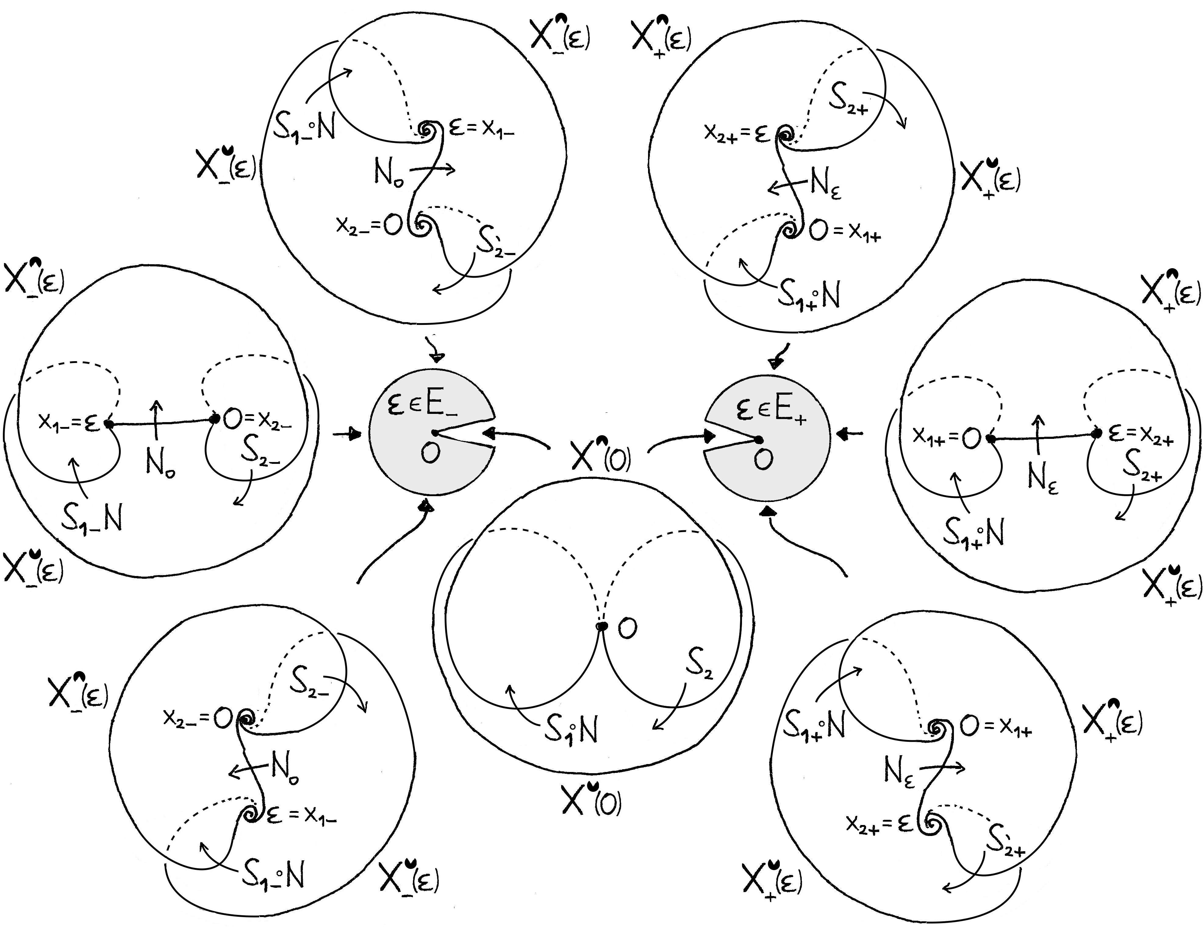
Figure 2: Sectoral isotropies connecting the canonical general solutions $y_{\pm}^{\bullet}$ depending on $\epsilon\in\mathsf{E}_{\pm}$.

Proposition 28 (Form of the Stokes isotropies).

Let $S_{i,\pm}(c,\epsilon)=\mskip 1.0mu\prescript{\smash{\mathrm{t}\mkern-3.0mu}}{}{\mathstrut(S_{1,i,\pm}(c,\epsilon),S_{2,i,\pm}(c,\epsilon))}$ be a Stokes sectoral isotropy (40). Then

• $S_{i,i,\pm}(c,\epsilon)=c_{i}+c_{i}^{2}\cdot\sigma_{i,i,\pm}(h,c_{i},\epsilon)$ for an analytic germ $\sigma_{i,i,\pm}$,

• $S_{j,i,\pm}(c,\epsilon)=c_{j}+\sigma_{j,i,\pm}(h,c_{i},\epsilon)$ for an analytic germ $\sigma_{j,i,\pm}$, $j=3-i$,

subject to a condition $\det D_{c}(S_{i,\pm})=1$.

The term $\sigma_{j,i,\pm}(0,0)$ is responsible for the ramification of the ramified center manifold $y=\mathbf{\Psi}_{\pm}(0,x,\epsilon)$ of the original vector field $Z_{\epsilon}$ at the sector $\mathsf{X}_{i,\pm}^{\cap}(\epsilon)$.

Proof.

The isotropy $\mathscr{S}_{i,\pm}(u,x,\epsilon)$ is analytic in $u$ on some neighborhood of $u=0$ and bounded in $x$ with $\lim_{x\to x_{i,\pm}}\mathscr{S}_{i,\pm}(u,x,\epsilon)=u$. By Lemma 24,

$$c_{i}\circ\mathscr{S}_{i,\pm}=c_{i}\cdot e^{f_{i}(h,c_{i},\epsilon)},\quad\text{and}\quad c_{j}\circ\mathscr{S}_{i,\pm}=c_{j}\cdot e^{f_{j}(h,\epsilon)}+g_{j}(h,c_{i},\epsilon)$$

where $f_{i},f_{j},g_{j}$ are some analytic functions of $(h,c_{i},\epsilon)$.

Knowing that $\lim_{x\to x_{i,\pm}}h\circ\mathscr{S}_{i,\pm}(u,x,\epsilon)=h$,

$$h\circ\mathscr{S}_{i,\pm}=h+c_{i}\cdot(\ldots),$$

where $(\ldots)$ is an analytic function of $(h,c_{i},\epsilon)$, which implies that $\lim_{x\to x_{i,\pm}}E_{\chi}^{-1}\cdot(E_{\chi}\circ h\circ\mathscr{S}_{i,\pm})=1$. Writing $\mathscr{S}_{i,\pm}=(\mathscr{S}_{1,i,\pm},\mathscr{S}_{2,i,\pm})$, its $k$-th component is

$$\mathscr{S}_{k,i,\pm}=\big{(}c_{k}\circ\mathscr{S}_{i,\pm}\big{)}\cdot\big{(}E^{-(-1)^{k}}\circ h\circ\mathscr{S}_{i,\pm}\big{)}.$$

We conclude that $f_{i}=c_{i}\cdot(\ldots)$ and $f_{j}=0$. ∎

4.5 Symmetry group of the system

Proposition 29.

The group of (analytic transversely symplectic fibered) symmetries of a system (1) is either

1. isomorphic to the exponential torus: this happens if and only if the system is analytically equivalent to the model (16), or

2. isomorphic to a finite cyclic group.

If the symmetry group is non-trivial, then the system has an analytic center manifold (bounded analytic solution on a neighborhood of both singular points).

Proof.

If $\Phi(y,x,\epsilon)$ is a symmetry of the system (1), then $\Phi(\cdot,x,\epsilon)\circ\mathbf{\Psi}_{\pm}(u,x,\epsilon)=\mathbf{\Psi}_{\pm}(\cdot,x,\epsilon)\circ\phi(u,\epsilon)$ for some germ

$$\phi:u\mapsto\left(\begin{smallmatrix}e^{a(h,\epsilon)}&\\ &e^{-a(h,\epsilon)}\end{smallmatrix}\right),$$

from the exponential torus, and the analyticity of $\Phi$ means that this $\phi$ must commute with the Stokes operators $S_{i,\pm}$ (40) (note that $\phi$ acts the same way on $c$ as on $u$). Using their characterization in Proposition 28, this means that

$$\sigma_{i1,\pm}(h,c_{1})=e^{a}\sigma_{i1,\pm}(h,e^{a}c_{1}),\qquad\sigma_{i2,\pm}(h,c_{2})=e^{-a}\sigma_{i2,\pm}(h,e^{-a}c_{2}),\quad i=1,2.$$

This can be satisfied only if

• either $\sigma_{ij,\pm}(h,c_{j})=0$ for all $i,j$, i.e. if $S_{1,\pm}=\mathrm{id}$, $S_{2,\pm}=\mathrm{id}$ and the system is analytically equivalent to its formal normal form,

• or there is $k\in\mathbb{N}$ such that $c_{j}\sigma_{ij,\pm}(h,c_{j})=0$ contains only powers of $c_{j}^{k}$ for all $i,j$, and $e^{ka}=1$, i.e. $a\in\frac{2\pi i}{k}\mathbb{Z}$.

∎

4.6 Analytic classification

Definition 30 (Analytic invariants).

The collection $(\chi,\{\mathscr{S}_{1,+},\mathscr{S}_{2,+},\mathscr{S}_{1,-},\mathscr{S}_{2,-}\})$ is called an analytic invariant of a system (1). Two analytic invariants $(\chi,\{\mathscr{S}_{i,\pm}\})$, $(\tilde{\chi},\{\tilde{\mathscr{S}}_{i,\pm}\})$ are equivalent if

• either $\chi=\tilde{\chi}$  and there is an element $\phi(u,\epsilon)$ of the exponential torus, analytic in $\epsilon$, such that: $\ \mathscr{S}_{i,\pm}=\phi\circ\tilde{\mathscr{S}}_{i,\pm}\circ\mathscr{\phi}^{\circ(-1)},\ i=1,2,$

• or $\chi(h,x,\epsilon)=-\tilde{\chi}(-h,x,\epsilon)$  and there is an element $\phi(u,\epsilon)$ of the exponential torus, analytic in $\epsilon$, such that: $\ \mathscr{S}_{i,\pm}=J\phi\circ\tilde{\mathscr{S}}_{j,\mp}\circ\mathscr{(}J\phi)^{\circ(-1)},\ i=1,2,\ j=3-i,$ where $J:(u_{1},u_{2})\mapsto(u_{2},-u_{1})$. Note that the definition of $\mathsf{E}_{\pm}$, $\mathsf{X}_{\pm}$ and $x_{i,\pm}$ depends on $\lambda(x,\epsilon)=\chi(0,x,\epsilon)$, therefore the relation $\tilde{\lambda}=-\lambda$ entails the renaming

  $$\tilde{\mathsf{E}}_{\pm}=\mathsf{E}_{\mp},\quad\tilde{\mathsf{X}}_{\pm}^{\bullet}=\mathsf{X}_{\mp}^{\bullet},\quad\tilde{x}_{i,\pm}=x_{j,\mp}.$$

By the construction, an analytic invariant of a system (1) is uniquely defined up to the equivalence.

Theorem 31 (Analytic classification).

Two systems (1) are analytically equivalent (in the sense of Definition 2) if and only if their analytic invariants are equivalent.

Proof.

If $y=\Phi(\tilde{y},x,\epsilon)$ is an analytic transformation from one system to another, then the sectoral normalizations $y=\mathbf{\Psi}_{\pm}(u,x,\epsilon)$ and $\tilde{y}=\tilde{\mathbf{\Psi}}_{\pm}(u,x,\epsilon)=\Phi\circ\mathbf{\Psi}_{\pm}$ provide the same analytic invariant. Conversely, if the analytic invariants are equivalent, then up to modifying one of the normalizing transformation, one can suppose that they are in fact equal, in which case $\Phi_{\pm}=\tilde{\mathbf{\Psi}}_{\pm}\circ\mathbf{\Psi}_{\pm}^{\circ(-1)}$ are analytic transformations between the systems on $\mathsf{E}_{+}$ and $\mathsf{E}_{-}$. In fact $\Phi_{+}=\Phi_{-}$ is an analytic on the whole $\epsilon$-neighborhood $\mathsf{E}$. Indeed, the composition $\Phi_{+}\circ\Phi_{-}^{\circ-1}$ is a symmetry of the second system on the intersection $\mathsf{E}_{+}\cap\mathsf{E}_{-}$, and as such it is determined by its value at $x=0$; but since $\tilde{\mathbf{\Psi}}_{+}\!\restriction_{x=0}=\tilde{\mathbf{\Psi}}_{-}\!\restriction_{x=0}=\tilde{\psi}^{(0)}(u,\epsilon)$ and ${\mathbf{\Psi}}_{+}\!\restriction_{x=0}={\mathbf{\Psi}}_{-}\!\restriction_{x=0}={\psi}^{(0)}(u,\epsilon)$ are analytic in $\epsilon$ (28), this means that $\Phi_{+}\circ\Phi_{-}^{\circ-1}\!\restriction_{x=0}=\mathrm{id}$ and therefore $\Phi_{+}\circ\Phi_{-}^{\circ-1}=\mathrm{id}$. ∎

4.7 Decomposition of monodromy operators

For $\epsilon\neq 0$, let $x_{0}\in\mathsf{X}_{\pm}(\epsilon)\smallsetminus\{0,\epsilon\}$ be a base-point, and let two counterclockwise simple loops around the singular points $x_{i,\pm}$, $i=1,2$, be as in Figure 3. Correspondingly, we have two monodromy operators $\mathfrak{M}_{x_{i,\pm}}$ acting on the foliation by the solutions of the original system (1) by analytic continuation along the loops. Since the monodromy operators $\mathfrak{M}_{x_{i,\pm}}$ act on the foliation, they are independent of the choice of the two-parameter general solution on which they act on the left (a different general solution is related to it by a change of the parameter, independent of $x$ and acting on the right). In particular

$$\mathfrak{M}_{x_{1,+}}\!=\mathfrak{M}_{x_{2,-}},\quad\mathfrak{M}_{x_{2,+}}\!=\mathfrak{M}_{x_{1,-}}.$$

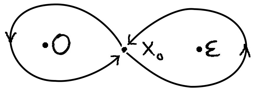
Figure 3: Simple loops along which the monodromy operators $\mathfrak{M}_{0}$ and $\mathfrak{M}_{\epsilon}$ are defined.

Theorem 32.

For $\epsilon\neq 0$, the monodromy operators $\mathfrak{M}_{x_{i,\pm}}$ of the original foliation are well defined on some open neighborhood of the ramified center manifold $y=\mathbf{\Psi}_{\pm}(0,x,\epsilon)$ in $\mathsf{Y}\times\mathsf{X}_{\pm}(\epsilon)$. Their (left) action is given by

$$\mathfrak{M}_{x_{i,\pm}}=\mathfrak{S}_{i,\pm}\circ\mathfrak{N}_{i,\pm},$$ (42)

where $\mathfrak{S}_{i,\pm}$ are the Stokes operators (41) and $\mathfrak{N}_{i,\pm}$ are the formal monodromy operators (37). Hence

$$\mathfrak{M}_{0} =\mathfrak{S}_{1,+}\circ\mathfrak{N}_{1,+}=\mathfrak{S}_{2,-}\circ\mathfrak{N}_{2,-},$$

$$\mathfrak{M}_{\epsilon} =\mathfrak{S}_{2,+}\circ\mathfrak{N}_{2,+}=\mathfrak{S}_{1,-}\circ\mathfrak{N}_{1,-}.$$

Their right action on analytic extension of the canonical general solutions $y_{\pm}^{\bullet}$ (33) to the whole $\mathsf{X}_{\pm}(\epsilon)$ is given by

$$\mathfrak{M}_{x_{i,\pm}}(y_{\pm}^{\bullet}(x,\epsilon;c),x,\epsilon)=y_{\pm}^{\bullet}(x,\epsilon;\cdot)\circ M_{i,\pm}^{\bullet}(c,\epsilon),\qquad\bullet=\scalebox{0.7}{\!$\mathrlap{\rotatebox[origin={c}]{-45.0}{$\LEFTCIRCLE$}}\rotatebox[origin={c}]{-135.0}{$\LEFTCIRCLE$}\!$},\scalebox{0.7}{\!$\mathrlap{\rotatebox[origin={c}]{45.0}{$\LEFTCIRCLE$}}\rotatebox[origin={c}]{135.0}{$\LEFTCIRCLE$}\!$},$$

where

$$M_{1,\pm}^{\scalebox{0.7}{\!$\mathrlap{\rotatebox[origin={c}]{-45.0}{$\LEFTCIRCLE$}}\rotatebox[origin={c}]{-135.0}{$\LEFTCIRCLE$}\!$}} =N_{x_{2,\pm}}^{\circ(-1)}\circ S_{1,\pm}\circ N, M_{1,\pm}^{\scalebox{0.7}{\!$\mathrlap{\rotatebox[origin={c}]{45.0}{$\LEFTCIRCLE$}}\rotatebox[origin={c}]{135.0}{$\LEFTCIRCLE$}\!$}} =S_{1,\pm}\circ N_{x_{1,\pm}},$$ (43)

$$M_{2,\pm}^{\scalebox{0.7}{\!$\mathrlap{\rotatebox[origin={c}]{-45.0}{$\LEFTCIRCLE$}}\rotatebox[origin={c}]{-135.0}{$\LEFTCIRCLE$}\!$}} =S_{2,\pm}\circ N_{x_{2,\pm}}, M_{2,\pm}^{\scalebox{0.7}{\!$\mathrlap{\rotatebox[origin={c}]{45.0}{$\LEFTCIRCLE$}}\rotatebox[origin={c}]{135.0}{$\LEFTCIRCLE$}\!$}} =N_{x_{2,\pm}}\circ S_{2,\pm},$$

cf. Figure 2.

Proof of Theorem 32.

The demonstration of the given formulas is straightforward, but we include it here for the sake of completeness. Let $\bar{x}:=x_{i,\pm}+e^{2\pi i}(x-x_{i,\pm})$, then

$$\mathfrak{M}_{x_{i,\pm}}(\cdot,x,\epsilon)\circ y_{\pm}(x,\epsilon;c) =y_{\pm}(\bar{x},\epsilon;c)=\mathbf{\Psi}_{\pm}(\cdot,\bar{x},\epsilon)\circ u(\bar{x},\epsilon;c)$$

$$=\big{(}\mathfrak{S}_{i,\pm}\circ\mathbf{\Psi}_{\pm}\big{)}(\cdot,x,\epsilon)\circ u(\bar{x},\epsilon;c)$$

$$=\big{(}\mathfrak{S}_{i,\pm}\circ\mathbf{\Psi}_{\pm}\circ\mathscr{N}_{i,\pm}\big{)}(\cdot,x,\epsilon)\circ u(x,\epsilon;c)$$

$$=\big{(}\mathfrak{S}_{i,\pm}\circ\mathfrak{N}_{i,\pm}\circ\mathbf{\Psi}_{\pm}\big{)}(\cdot,x,\epsilon)\circ u(x,\epsilon;c)$$

$$=\big{(}\mathfrak{S}_{i,\pm}\circ\mathfrak{N}_{i,\pm}\circ y_{\pm}\big{)}(x,\epsilon;c),$$

using (41), (34), (37). Similarly, to calculate $M_{1,\pm}^{\scalebox{0.7}{\!$\mathrlap{\rotatebox[origin={c}]{-45.0}{$\LEFTCIRCLE$}}\rotatebox[origin={c}]{-135.0}{$\LEFTCIRCLE$}\!$}}$ for example,

$$y_{\pm}^{\scalebox{0.7}{\!$\mathrlap{\rotatebox[origin={c}]{-45.0}{$\LEFTCIRCLE$}}\rotatebox[origin={c}]{-135.0}{$\LEFTCIRCLE$}\!$}}(\bar{x},\epsilon;c) =\mathbf{\Psi}_{\pm}(\cdot,\bar{x},\epsilon)\circ u^{\scalebox{0.7}{\!$\mathrlap{\rotatebox[origin={c}]{-45.0}{$\LEFTCIRCLE$}}\rotatebox[origin={c}]{-135.0}{$\LEFTCIRCLE$}\!$}}(\bar{x},\epsilon;c)$$

$$=\mathbf{\Psi}_{\pm}(\cdot,\bar{x},\epsilon)\circ u^{\scalebox{0.7}{\!$\mathrlap{\rotatebox[origin={c}]{45.0}{$\LEFTCIRCLE$}}\rotatebox[origin={c}]{135.0}{$\LEFTCIRCLE$}\!$}}(\bar{x},\epsilon;\cdot)\circ N_{x_{2,\pm}}(c,\epsilon)$$

$$=\mathbf{\Psi}_{\pm}(\cdot,\bar{x},\epsilon)\circ u^{\scalebox{0.7}{\!$\mathrlap{\rotatebox[origin={c}]{45.0}{$\LEFTCIRCLE$}}\rotatebox[origin={c}]{135.0}{$\LEFTCIRCLE$}\!$}}(x,\epsilon;\cdot)\circ N_{x_{1,\pm}}\circ N_{x_{2,\pm}}(c,\epsilon)$$

$$=\mathbf{\Psi}_{\pm}(\cdot,x,\epsilon)\circ u^{\scalebox{0.7}{\!$\mathrlap{\rotatebox[origin={c}]{45.0}{$\LEFTCIRCLE$}}\rotatebox[origin={c}]{135.0}{$\LEFTCIRCLE$}\!$}}(x,\epsilon;\cdot)\circ S_{1,\pm}\circ N_{x_{1,\pm}}\circ N_{x_{2,\pm}}(c,\epsilon)$$

$$=\mathbf{\Psi}_{\pm}(\cdot,x,\epsilon)\circ u^{\scalebox{0.7}{\!$\mathrlap{\rotatebox[origin={c}]{-45.0}{$\LEFTCIRCLE$}}\rotatebox[origin={c}]{-135.0}{$\LEFTCIRCLE$}\!$}}(x,\epsilon;\cdot)\circ N_{x_{2,\pm}}^{\circ(-1)}\circ S_{1,\pm}\circ N_{x_{1,\pm}}\circ N_{x_{2,\pm}}(c,\epsilon)$$

$$=y_{\pm}^{\scalebox{0.7}{\!$\mathrlap{\rotatebox[origin={c}]{-45.0}{$\LEFTCIRCLE$}}\rotatebox[origin={c}]{-135.0}{$\LEFTCIRCLE$}\!$}}(x,\epsilon;\cdot)\circ N_{x_{2,\pm}}^{\circ(-1)}\circ S_{1,\pm}\circ N(c,\epsilon),$$

see Figure 2. The general solutions $y_{\pm}^{\scalebox{0.7}{\!$\mathrlap{\rotatebox[origin={c}]{-45.0}{$\LEFTCIRCLE$}}\rotatebox[origin={c}]{-135.0}{$\LEFTCIRCLE$}\!$}},\ y_{\pm}^{\scalebox{0.7}{\!$\mathrlap{\rotatebox[origin={c}]{45.0}{$\LEFTCIRCLE$}}\rotatebox[origin={c}]{135.0}{$\LEFTCIRCLE$}\!$}}$ are related by

$$y_{\pm}^{\scalebox{0.7}{\!$\mathrlap{\rotatebox[origin={c}]{-45.0}{$\LEFTCIRCLE$}}\rotatebox[origin={c}]{-135.0}{$\LEFTCIRCLE$}\!$}}(x,\epsilon;c)=y_{\pm}^{\scalebox{0.7}{\!$\mathrlap{\rotatebox[origin={c}]{45.0}{$\LEFTCIRCLE$}}\rotatebox[origin={c}]{135.0}{$\LEFTCIRCLE$}\!$}}(x,\epsilon;\cdot)\circ N_{x_{2,\pm}}(c,\epsilon).$$

∎

Note that in general, a composition of the two monodromies may not be defined if the image of the first does not intersect the domain of definition the second.

4.8 Accumulation of monodromy

Definition 33 (Monodromy pseudogroup).

1. For $\epsilon\neq 0$, the pseudogroup generated by the monodromy operators

   $$\langle\mathfrak{M}_{0}(\cdot,x,\epsilon),\ \mathfrak{M}_{\epsilon}(\cdot,x,\epsilon)\rangle$$

   is called the (local) monodromy pseudogroup. The pseudogroup generated by the corresponding action on the initial condition $c$

   $$\langle M_{1,\pm}^{\bullet}(\cdot,\epsilon),\ M_{2,\pm}^{\bullet}(\cdot,\epsilon)\rangle$$

   is its representation with respect to the general solution $y_{\pm}^{\bullet}(x,\epsilon;c)$.

2. For $\epsilon=0$, the pseudogroup generated by the Stokes operators and by the elements of the exponential torus (pushed-forward by the sectoral transformations $\mathbf{\Psi}^{\bullet}$):

   $$\langle\mathfrak{S}_{1,\pm}(\cdot,x,0),\ \mathfrak{S}_{2,\pm}(\cdot,x,0),\ \{\mathfrak{T}_{a}^{\bullet}(\cdot,x,0)\}_{a}\rangle,$$

   where $\mathfrak{T}_{a}^{\bullet}(\cdot,x,0)=\mathbf{\Psi}_{\pm}^{\bullet}(\cdot,x,0)_{*}\mathcal{T}_{a}=\Phi^{1}_{(\mathbf{\Psi}_{\pm}^{\bullet})_{*}(a(h)X_{h})}$, is called the (local) wild monodromy pseudogroup. The pseudogroup generated by the corresponding action on the initial condition $c$

   $$\langle S_{1,\pm}(\cdot,0),\ S_{2,\pm}(\cdot,0),\ \{\mathcal{T}_{a}(\cdot)\}_{a}\rangle,$$ (44)

   is its representation with respect to the formal transseries solution $\hat{y}(x,0;c)=\hat{\mathbf{\Psi}}(u(x,0;c),x,0)$.

Note that the pseudogroup (44) is independent of the freedom of choice of the sectoral normalizations $\mathbf{\Psi}_{\pm}^{\bullet}$ of Theorem 13.

One of the main goals of this paper is to understand the relation between the monodromy pseudogroup for $\epsilon\neq 0$ and the wild monodromy pseudogroup for $\epsilon=0$.

Suppose that the formal invariant $\chi(h,x,\epsilon)$ is such that

$$\chi(h,x,0)=\lambda^{(0)}(0)+x\chi^{(1)}(h,0),$$ (45)

and therefore

$$\chi(h,x,\epsilon)=\lambda^{(0)}(0)+\epsilon\tfrac{\partial\chi^{(0)}}{\partial\epsilon}(h,0)+x\chi^{(1)}(h,0)+O(x\epsilon)+O(\epsilon^{2}).$$

Let $\{\epsilon_{n}\}_{n\in\pm\mathbb{N}}$ be sequence in $\mathsf{E}_{\pm}\smallsetminus\{0\}$ defined by

$$\tfrac{\lambda^{(0)}(0)}{\epsilon_{n}}=\tfrac{\lambda^{(0)}(0)}{\epsilon_{0}}+n,\qquad\epsilon_{0}\in\mathsf{E}_{\pm}\smallsetminus\{0\}$$ (46)

along which the exponential factor $e^{\frac{2\pi i\lambda^{(0)}}{\epsilon}}$ in the formal monodromy (36) stays constant, and denote

$$\kappa:=e^{\frac{2\pi i\lambda^{(0)}}{\epsilon_{0}}}.$$ (47)

Then the formal monodromy operators $\mathscr{N}_{0}(u,x,\epsilon),\mathscr{N}_{\epsilon}(u,x,\epsilon)$, resp. $N_{0}(u,x,\epsilon),N_{\epsilon}(u,x,\epsilon)$, converge along each such sequence to a symmetry of the model system (element of the exponential torus)

$$\hskip-6.0pt\tilde{N}_{0}(\kappa;u,x):=\!\!\lim_{n\to\pm\infty\!\!}\!\!N_{0}(u,x,\epsilon_{n}) :\ c\mapsto\left(\!\!\begin{smallmatrix}\kappa^{-1}e^{-2\pi i\frac{\partial\chi^{(0)}}{\partial\epsilon}(h,0)}&0\\ 0&\kappa e^{2\pi i\frac{\partial\chi^{(0)}}{\partial\epsilon}(h,0)}\end{smallmatrix}\!\right)c,$$ (48)

$$\hskip-6.0pt\tilde{N}_{\epsilon}(\kappa;u,x):=\!\!\lim_{n\to\pm\infty\!\!}\!\!N_{\epsilon}(u,x,\epsilon_{n}) :\ c\mapsto\left(\!\!\begin{smallmatrix}\kappa e^{2\pi i[\frac{\partial\chi^{(0)}}{\partial\epsilon}(h,0)+\chi^{(1)}(h,0)]}\hskip-15.0pt&0\\ 0&\hskip-15.0pt\kappa^{-1}e^{-2\pi i[\frac{\partial\chi^{(0)}}{\partial\epsilon}(h,0)+\chi^{(1)}(h,0)]}\end{smallmatrix}\!\right)c,\hskip-6.0pt$$

$\kappa\in\mathbb{C}^{*}$. This implies that also the monodromy operators $M_{i,\pm}^{\cdot}(c,\epsilon)$, resp. $\mathfrak{M}_{x_{i,\pm}}(y,x,\epsilon)$, converge along such sequences $\{\epsilon_{n}\}_{n\in\pm\mathbb{N}}\subset\mathsf{E}_{\pm}\smallsetminus\{0\}$. Denote

$$\tilde{\mathfrak{N}}_{{i,\pm}}^{\bullet}(\kappa;y,x):=\lim_{n\to\pm\infty}\mathfrak{N}_{{i,\pm}}(y,x,\epsilon_{n}),\qquad x\in\mathsf{X}_{\pm}^{\bullet},\quad\bullet=\scalebox{0.7}{\!$\mathrlap{\rotatebox[origin={c}]{-45.0}{$\LEFTCIRCLE$}}\rotatebox[origin={c}]{-135.0}{$\LEFTCIRCLE$}\!$},\scalebox{0.7}{\!$\mathrlap{\rotatebox[origin={c}]{45.0}{$\LEFTCIRCLE$}}\rotatebox[origin={c}]{135.0}{$\LEFTCIRCLE$}\!$}.$$

Theorem 34.

Suppose that the formal invariant of the form (45). Then the monodromy operators of the system (1) for $\epsilon\neq 0$ accumulate along the sequences $\{\epsilon_{n}\}_{n\in\pm\mathbb{N}}$ (46) to a 1-parameter family of wild monodromy operators

$$\tilde{\mathfrak{M}}_{1,\pm}(\kappa;y,x):=\lim_{n\to\pm\infty}\mathfrak{M}_{x_{1,\pm}}(y,x,\epsilon_{n}) =\mathfrak{S}_{1,\pm}(\cdot,x,0)\circ\tilde{\mathfrak{N}}_{x_{1,\pm}}^{\scalebox{0.7}{\!$\mathrlap{\rotatebox[origin={c}]{45.0}{$\LEFTCIRCLE$}}\rotatebox[origin={c}]{135.0}{$\LEFTCIRCLE$}\!$}}(\kappa;y,x),\qquad x\in\mathsf{X}^{\cap}_{1,\pm}(0),$$

$$\tilde{\mathfrak{M}}_{2,\pm}(\kappa;y,x):=\lim_{n\to\pm\infty}\mathfrak{M}_{x_{2,\pm}}(y,x,\epsilon_{n}) =\mathfrak{S}_{2,\pm}(\cdot,x,0)\circ\tilde{\mathfrak{N}}_{x_{2,\pm}}^{\scalebox{0.7}{\!$\mathrlap{\rotatebox[origin={c}]{-45.0}{$\LEFTCIRCLE$}}\rotatebox[origin={c}]{-135.0}{$\LEFTCIRCLE$}\!$}}(\kappa;y,x),\qquad x\in\mathsf{X}^{\cap}_{2,\pm}(0).$$

In particular, if we replace $\kappa$ by $e^{-2\pi i\big{[}\frac{\partial\chi^{(0)}}{\partial\epsilon}(h,0)+\delta_{i,\pm}(0)\chi^{(1)}(h,0)\big{]}}$, $\delta_{i,\pm}(\epsilon)=\frac{x_{i,\pm}(\epsilon)}{\epsilon}$, so that $\tilde{\mathfrak{N}}_{x_{i,\pm}}^{\bullet}(\kappa;y,x)$ becomes an identity, we obtain the Stokes operators

$$\mathfrak{S}_{i,\pm}(y,x,0)=\tilde{\mathfrak{M}}_{i,\pm}(e^{-2\pi i\big{[}\frac{\partial\chi^{(0)}}{\partial\epsilon}(h,0)+\delta_{i,\pm}(0)\chi^{(1)}(h,0)\big{]}};y,x).$$ (49)

The vector field

$$\dot{y}=\pm(-1)^{i}\big{(}\kappa\tfrac{\partial}{\partial\kappa}\tilde{\mathfrak{M}}_{i,\pm}(\kappa;y,x)^{\circ(-1)}\big{)}\circ\tilde{\mathfrak{M}}_{i,\pm}(\kappa;y,x)$$ (50)

equals to the push-forward $\mathbf{\Psi}_{\pm}^{\bullet}(\cdot,x,0)_{*}\big{(}X_{h}\big{)}$ of the vector field $X_{h}=u_{1}\partial_{u_{1}}-u_{2}\partial_{u_{2}}$, where $\bullet=\scalebox{0.7}{\!$\mathrlap{\rotatebox[origin={c}]{45.0}{$\LEFTCIRCLE$}}\rotatebox[origin={c}]{135.0}{$\LEFTCIRCLE$}\!$}$ if $i=1$ and $\bullet=\scalebox{0.7}{\!$\mathrlap{\rotatebox[origin={c}]{-45.0}{$\LEFTCIRCLE$}}\rotatebox[origin={c}]{-135.0}{$\LEFTCIRCLE$}\!$}$ if $i=2$, which “generates” the commutative Lie algebra of bounded infinitesimal symmetries on the sector $\mathsf{X}^{\bullet}(0)$.

Conclusion.

The knowledge of the limits $\tilde{\mathfrak{M}}_{i,\pm}(\kappa;y,x)$, $\kappa\in\mathbb{C}^{*}$, allows to recover the infinitesimal symmetry $\mathbf{\Psi}_{\pm}^{\bullet}(\cdot,x,0)_{*}\big{(}X_{h}\big{)}$ (50), and hence its Hamiltonian, the bounded first integral $\mathbf{\Psi}_{\pm}^{\bullet}(\cdot,x,0)_{*}(h)$ which vanishes at the singular points $(y_{0}(x_{i,\pm},\epsilon),x_{i,\pm})$, and therefore, knowing the formal invariant $\chi$, also the formal monodromy operators $\tilde{\mathfrak{N}}_{x_{1,\pm}}^{\bullet}(\kappa;y,x)$, and finally the Stokes isotropies $\mathfrak{S}_{i,\pm}(y,x,0)$.

Remark 35.

In the case when the assumption (45) is not met, one can nevertheless get a similar “accumulation” result by replacing in (46) $\lambda^{(0)}(0)$ by $\chi(h,0,0)$ and defining $\kappa(h)=e^{\frac{2\pi i\chi(h,0,0)}{\epsilon_{0}(h)}}$ (47).

5 Confluence in $2\!\times\!2$ traceless linear systems and their differential Galois group

To illustrate the matter of the previous section, let us consider a confluence of two regular singular points to a non-resonant irregular singular point in a family of linear systems

$$x(x-\epsilon)\frac{dy}{dx}=A(x,\epsilon)y,\qquad y\in\mathbb{C}^{2},$$ (51)

where $A$ is a $2\!\times\!2$ traceless complex matrix depending analytically on $(x,\epsilon)\in(\mathbb{C}\!\times\!\mathbb{C},0)$, such that $A(0,0)\neq 0$ has two distinct eigenvalues $\pm\lambda^{(0)}(0)$.

The Theorem 14 in this case can be found in the thesis of Parise [Par01] and in the work of Lambert and Rousseau [LR12] (see also [HLR13]). It provides us with a canonical fundamental solution matrices

$$Y_{\pm}^{\bullet}(x,\epsilon)=\mathbf{\Psi}_{\pm}(x,\epsilon)\cdot U_{\pm}^{\bullet}(x,\epsilon),\qquad\bullet=\scalebox{0.7}{\!$\mathrlap{\rotatebox[origin={c}]{-45.0}{$\LEFTCIRCLE$}}\rotatebox[origin={c}]{-135.0}{$\LEFTCIRCLE$}\!$},\scalebox{0.7}{\!$\mathrlap{\rotatebox[origin={c}]{45.0}{$\LEFTCIRCLE$}}\rotatebox[origin={c}]{135.0}{$\LEFTCIRCLE$}\!$},$$ (52)

where the transformation matrix $\mathbf{\Psi}_{\pm}(x,\epsilon)$ is bounded on $\mathsf{XE}_{\pm}$, and

$$U_{\pm}^{\bullet}(x,\epsilon)=\left(\begin{smallmatrix}E_{\lambda}^{\bullet}(x,\epsilon)&0\\ 0&E_{\lambda}^{\bullet}(x,\epsilon)^{-1}\end{smallmatrix}\right),$$ (53)

is a solution to the diagonal model system

$$x(x-\epsilon)\frac{dy}{dx}=\left(\begin{smallmatrix}\lambda(x,\epsilon)&\\ &-\lambda(x,\epsilon)\end{smallmatrix}\right)y.$$

The solution basis $Y_{\pm}^{\bullet}(x,\epsilon)$ is also called a mixed basis: the first (resp. second) column spans the subspace of solutions that asymptotically vanish when $x\to x_{1,\pm}(\epsilon)$ (resp. when $x\to x_{2,\pm}(\epsilon)$), and it is an eigensolution with respect to the corresponding monodromy operator $\mathfrak{M}_{x_{1,\pm}}$ (resp. $\mathfrak{M}_{x_{2,\pm}}$) associated to its eigenvalue $e^{\pm 2\pi i\frac{\lambda(x_{1,\pm},\epsilon)}{\epsilon}}$ (resp. $e^{\pm 2\pi i\frac{\lambda(x_{2,\pm},\epsilon)}{\epsilon}}$). A general solution is a linear combination

$$y_{\pm}^{\bullet}(x,\epsilon;c)=Y_{\pm}^{\bullet}(x,\epsilon)\cdot c,\qquad\bullet=\scalebox{0.7}{\!$\mathrlap{\rotatebox[origin={c}]{-45.0}{$\LEFTCIRCLE$}}\rotatebox[origin={c}]{-135.0}{$\LEFTCIRCLE$}\!$},\scalebox{0.7}{\!$\mathrlap{\rotatebox[origin={c}]{45.0}{$\LEFTCIRCLE$}}\rotatebox[origin={c}]{135.0}{$\LEFTCIRCLE$}\!$}.$$

Let $\mathbb{K}$ be the field of meromorphic functions of the variable $x$ on a fixed small neighborhood of $0$, equipped with the differentiation $\frac{d}{dx}$. For a fixed small $\epsilon$, the local differential Galois group (also called the Picard-Vessiot group) of the system (51) is the group of $\mathbb{K}$-automorphisms of the differential field $\mathbb{K}\langle Y(\cdot,\epsilon)\rangle$, generated by the components of any fundamental matrix solution $Y(x,\epsilon)$. The differential Galois group acts on the foliation associated to the system by left multiplication. Fixing a fundamental solution matrix $Y=Y_{\pm}^{\bullet}$, then each automorphism is represented by a right multiplication of $Y_{\pm}^{\bullet}$ by a constant invertible matrix, hence the differential Galois group is represented by an (algebraic) subgroup of $\mathrm{SL}_{2}(\mathbb{C})$ acting on the right.

It is well known [MR91, SP03] that the differential Galois group is the Zariski closure of

• the monodromy group generated by the two monodromy operators around the singular points $0$ and $\epsilon$,

• the wild monodromy group generated by the Stokes operators and the linear exponential torus  which acts on the fundamental solutions $Y_{\pm}^{\bullet}$ as

  $$\mathfrak{T}_{a}^{\bullet}:Y_{\pm}^{\bullet}(x,0)\mapsto Y_{\pm}^{\bullet}(x,0)\cdot T_{a},\quad\text{where}\quad T_{a}=\left(\begin{smallmatrix}e^{a}&\\ &e^{-a}\end{smallmatrix}\right),\quad a\in\mathbb{C}.$$ (54)

The question is how are these two different descriptions related?

The monodromy matrices of $Y_{\pm}^{\scalebox{0.7}{\!$\mathrlap{\rotatebox[origin={c}]{-45.0}{$\LEFTCIRCLE$}}\rotatebox[origin={c}]{-135.0}{$\LEFTCIRCLE$}\!$}},\ Y_{\pm}^{\scalebox{0.7}{\!$\mathrlap{\rotatebox[origin={c}]{45.0}{$\LEFTCIRCLE$}}\rotatebox[origin={c}]{135.0}{$\LEFTCIRCLE$}\!$}}$, around the points $x_{1,\pm}(\epsilon)$, $x_{2,\pm}(\epsilon)$, $\epsilon\in\mathsf{E}_{\pm}\smallsetminus\{0\}$, are given respectively by

$$M_{1,\pm}^{\scalebox{0.7}{\!$\mathrlap{\rotatebox[origin={c}]{-45.0}{$\LEFTCIRCLE$}}\rotatebox[origin={c}]{-135.0}{$\LEFTCIRCLE$}\!$}} =N_{x_{2,\pm}}^{(-1)}S_{1,\pm}N, M_{2,\pm}^{\scalebox{0.7}{\!$\mathrlap{\rotatebox[origin={c}]{-45.0}{$\LEFTCIRCLE$}}\rotatebox[origin={c}]{-135.0}{$\LEFTCIRCLE$}\!$}} =S_{2,\pm}N_{x_{2,\pm}}$$

$$M_{1,\pm}^{\scalebox{0.7}{\!$\mathrlap{\rotatebox[origin={c}]{45.0}{$\LEFTCIRCLE$}}\rotatebox[origin={c}]{135.0}{$\LEFTCIRCLE$}\!$}} =S_{1,\pm}N_{x_{1,\pm}}, M_{2,\pm}^{\scalebox{0.7}{\!$\mathrlap{\rotatebox[origin={c}]{45.0}{$\LEFTCIRCLE$}}\rotatebox[origin={c}]{135.0}{$\LEFTCIRCLE$}\!$}} =N_{x_{2,\pm}}S_{2,\pm},$$

where $S_{i,\pm}$ are of the form

$$S_{1,\pm}=\left(\begin{smallmatrix}1&0\\[3.0pt] s_{1,\pm}&1\end{smallmatrix}\right),\qquad S_{2,\pm}=\left(\begin{smallmatrix}1&s_{2,\pm}\\[3.0pt] 0&1\end{smallmatrix}\right).$$

In particular $M_{1,\pm}^{\bullet}$ is lower-triangular and $M_{2,\pm}^{\bullet}$ is upper-triangular.

When $\epsilon\to 0$ along a sequence $\frac{1}{\epsilon_{n}}=\frac{1}{\epsilon_{0}}+\frac{n}{\lambda^{(0)}}$, $n\in\pm\mathbb{N}$, $\epsilon_{0}\in\mathsf{E}_{\pm}\smallsetminus\{0\}$, these monodromy converge respectively to $\tilde{M}_{i,\pm}^{\bullet}(\kappa)=\lim_{n\to\pm\infty}M_{i,\pm}^{\bullet}(\epsilon_{n})$ given by

$$\tilde{M}_{1,+}^{\scalebox{0.7}{\!$\mathrlap{\rotatebox[origin={c}]{-45.0}{$\LEFTCIRCLE$}}\rotatebox[origin={c}]{-135.0}{$\LEFTCIRCLE$}\!$}}(\kappa) =\tilde{N}_{\epsilon}(\kappa)^{-1}S_{1}(0)N(0), \tilde{M}_{1,+}^{\scalebox{0.7}{\!$\mathrlap{\rotatebox[origin={c}]{45.0}{$\LEFTCIRCLE$}}\rotatebox[origin={c}]{135.0}{$\LEFTCIRCLE$}\!$}}(\kappa) =S_{1}(0)\tilde{N}_{0}(\kappa),$$

$$\tilde{M}_{2,+}^{\scalebox{0.7}{\!$\mathrlap{\rotatebox[origin={c}]{-45.0}{$\LEFTCIRCLE$}}\rotatebox[origin={c}]{-135.0}{$\LEFTCIRCLE$}\!$}}(\kappa) =S_{2}(0)\tilde{N}_{\epsilon}(\kappa), \tilde{M}_{2,+}^{\scalebox{0.7}{\!$\mathrlap{\rotatebox[origin={c}]{45.0}{$\LEFTCIRCLE$}}\rotatebox[origin={c}]{135.0}{$\LEFTCIRCLE$}\!$}}(\kappa) =\tilde{N}_{\epsilon}(\kappa)S_{2}(0),$$

$$\tilde{M}_{1,-}^{\scalebox{0.7}{\!$\mathrlap{\rotatebox[origin={c}]{-45.0}{$\LEFTCIRCLE$}}\rotatebox[origin={c}]{-135.0}{$\LEFTCIRCLE$}\!$}}(\kappa) =\tilde{N}_{0}(\kappa)^{-1}S_{1}(0)N(0), \tilde{M}_{1,-}^{\scalebox{0.7}{\!$\mathrlap{\rotatebox[origin={c}]{45.0}{$\LEFTCIRCLE$}}\rotatebox[origin={c}]{135.0}{$\LEFTCIRCLE$}\!$}}(\kappa) =S_{1}(0)\tilde{N}_{\epsilon}(\kappa),$$

$$\tilde{M}_{2,-}^{\scalebox{0.7}{\!$\mathrlap{\rotatebox[origin={c}]{-45.0}{$\LEFTCIRCLE$}}\rotatebox[origin={c}]{-135.0}{$\LEFTCIRCLE$}\!$}}(\kappa) =S_{2}(0)\tilde{N}_{0}(\kappa), \tilde{M}_{2,-}^{\scalebox{0.7}{\!$\mathrlap{\rotatebox[origin={c}]{45.0}{$\LEFTCIRCLE$}}\rotatebox[origin={c}]{135.0}{$\LEFTCIRCLE$}\!$}}(\kappa) =\tilde{N}_{0}(\kappa)S_{2}(0),$$

with

$$\tilde{N}_{0}(\kappa)=\left(\begin{smallmatrix}\kappa^{-1}&\\[3.0pt] &\kappa\end{smallmatrix}\right)T_{-2\pi i\frac{d\lambda^{(0)}}{d\epsilon}(0)},\quad\tilde{N}_{\epsilon}(\kappa)=\left(\begin{smallmatrix}\kappa&\\[3.0pt] &\kappa^{-1}\end{smallmatrix}\right)T_{2\pi i[\frac{d\lambda^{(0)}}{d\epsilon}(0)+\lambda^{(1)}(0)]},\quad N(0)=T_{2\pi i\lambda^{(1)}(0)}.$$

We call them wild monodromy matrices. The family of them

$$\{\tilde{M}_{1,\pm}^{\bullet}(\kappa),\ \tilde{M}_{2,\pm}^{\bullet}(\kappa)\ |\ \kappa\in\mathbb{C}^{*}\}$$

generates the same group, the representation of the wild monodromy group with respect to the formal solution $\hat{Y}(x,\epsilon)$, as does the collection of the Stokes matrices and the linear exponential torus

$$\{S_{1}(0),S_{2}(0)\}\cup\{T_{a}\ |\ a\in\mathbb{C}\}.$$

Hence we have the following theorem, whose general idea was suggested by J.-P. Ramis [Ram89]:

Theorem 36.

When $\epsilon\to 0$ the elements of the monodromy group of the system (51) accumulate to generators of the wild monodromy group of the limit system.

6 Confluent degeneration of the sixth Painlevé equation to the fifth

The sixth Painlevé equation is

$$\begin{split}P_{VI}:\ \ q^{\prime\prime}&=\frac{1}{2}\Big{(}\frac{1}{q}+\frac{1}{q-1}+\frac{1}{q-t}\Big{)}(q^{\prime})^{2}-\Big{(}\frac{1}{t}+\frac{1}{t-1}+\frac{1}{q-t}\Big{)}q^{\prime}\\ &\ +\frac{q(q-1)(q-t)}{2\,t^{2}(t-1)^{2}}\Big{[}(\vartheta_{\infty}\!-\!1)^{2}-\vartheta_{0}^{2}\frac{t}{q^{2}}+\vartheta_{1}^{2}\frac{(t-1)}{(q-1)^{2}}+(1\!-\!\vartheta_{t}^{2})\frac{t(t-1)}{(q-t)^{2}}\Big{]},\end{split}$$

where $\vartheta=(\vartheta_{0},\vartheta_{t},\vartheta_{1},\vartheta_{\infty})\in\mathbb{C}^{4}$ are complex constants. It is a reduction to the $q$-variable of a time dependent Hamiltonian system [Oka80]

$$\frac{dq}{dt}=\,\frac{\partial H_{VI}(q,p,t)\!}{\partial p},\qquad\frac{dp}{dt}=-\frac{\partial H_{VI}(q,p,t)}{\partial q},$$ (55)

with a polynomial Hamiltonian function

$$\begin{split}H_{VI}=\tfrac{1}{t(t-1)}\Big{[}&q(q-1)(q-t)p^{2}-\Big{(}\vartheta_{0}(q-1)(q-t)+\vartheta_{1}q(q-t)+(\vartheta_{t}-1)q(q-1)\Big{)}p\\ &+\tfrac{(\vartheta_{0}+\vartheta_{1}+\vartheta_{t}-1)^{2}-\vartheta_{\infty}^{2}}{4}(q-t)\Big{]}.\end{split}$$

It has three simple (regular) singular points on the Riemann sphere $\mathbb{CP}^{1}$ at $t=0,1,\infty$.

The fifth Painlevé equation $P_{V}$ 

$$P_{V}:\ \ q^{\prime\prime}=\Big{(}\frac{1}{2q}+\frac{1}{q\!-\!1}\Big{)}(q^{\prime})^{2}-\frac{1}{\tilde{t}}q^{\prime}+\frac{(q\!-\!1)^{2}}{2\tilde{t}^{2}}\Big{(}(\vartheta_{\infty}\!-1)^{2}q-\frac{\vartheta_{0}^{2}}{q}\Big{)}+(1+\tilde{\vartheta}_{1})\frac{q}{\tilde{t}}-\frac{q(q\!+\!1)}{2(q\!-\!1)},$$

is obtained from $P_{VI}$ as a limit $\epsilon\to 0$ after the change of the independent variable

$$t=1+\epsilon\tilde{t},\qquad\vartheta_{t}=\frac{1}{\epsilon},\quad\vartheta_{1}=-\frac{1}{\epsilon}+\tilde{\vartheta}_{1}+1,$$ (56)

which sends the three singularities to $\tilde{t}=-\frac{1}{\epsilon},0,\infty$. At the limit, the two simple singular points $-\frac{1}{\epsilon}$ and $\infty$ merge into a double (irregular) singularity at the infinity.

The change of variables (56), changes the function $\epsilon\cdot H_{VI}$ to

$$\begin{split}H_{VI,\epsilon}=\tfrac{1}{\tilde{t}(1+\epsilon\tilde{t})}\Big{[}&q(q-1)(q-1-\epsilon\tilde{t})p^{2}-\Big{(}\vartheta_{0}(q-1)(q-1-\epsilon\tilde{t})+\tilde{\vartheta}_{1}q(q-1-\epsilon\tilde{t})+\tilde{t}q-\epsilon\tilde{t}q\Big{)}p\\ &+\tfrac{(\vartheta_{0}+\tilde{\vartheta}_{1})^{2}-\vartheta_{\infty}^{2}}{4}(q-1-\epsilon\tilde{t})\Big{]},\end{split}$$

and the Hamiltonian system to

$$\frac{dq}{d\tilde{t}}=\,\frac{\partial H_{VI,\epsilon}(q,p,\tilde{t})}{\partial p},\qquad\frac{dp}{d\tilde{t}}=-\frac{\partial H_{VI,\epsilon}(q,p,\tilde{t})}{\partial q},$$

whose limit $\epsilon\to 0$ is a Hamiltonian system of $P_{V}$. In the coordinate $x=\frac{1}{\tilde{t}}+\epsilon$, the above system is written as

$$x(x-\epsilon)\frac{dq}{dx}=\,\frac{\partial H(q,p,x,\epsilon)\!}{\partial p},\qquad x(x-\epsilon)\frac{dp}{dx}=-\frac{\partial H(q,p,x,\epsilon)\!}{\partial q},$$ (57)

with

$$H(q,p,x,\epsilon) =-(1+\epsilon\tilde{t})H_{VI,\epsilon}(q,p,\tilde{t})$$

$$=-\tfrac{(\vartheta_{0}+\tilde{\vartheta}_{1})^{2}-\vartheta_{\infty}^{2}}{4}((x-\epsilon)q-x)+x\vartheta_{0}p+\big{(}1-\epsilon-(x-\epsilon)\vartheta_{0}-x(\vartheta_{0}+\tilde{\vartheta}_{1})\big{)}qp$$

$$\qquad+(2x-\epsilon)(qp)^{2}+(x-\epsilon)(\theta_{0}+\tilde{\vartheta}_{1})q^{2}p-xqp^{2}-(x-\epsilon)q^{3}p^{2},$$

and Theorem 14 can be applied.

Theorem 37.

The formal invariant $\chi$ of the system (57) is

$$\chi(h,x,\epsilon)=1-\epsilon-(x-\epsilon)\vartheta_{0}-x(\vartheta_{0}+\tilde{\vartheta}_{1})+2(2x-\epsilon)h.$$ (58)

Proof.

Let

$$\tilde{q} =q-xA, \qquad A =\tfrac{\vartheta_{0}}{1+\epsilon(1+\vartheta_{0}+\tilde{\vartheta}_{1})},\qquad$$

$$\tilde{p} =p+(x-\epsilon)B, B =\tfrac{(\vartheta_{0}+\tilde{\vartheta}_{1})^{2}-\vartheta_{\infty}^{2}}{4(1+\epsilon(1-\vartheta_{0}))},$$

and let

$$\tilde{H}(\tilde{q},\tilde{p},x,\epsilon)=H(q,p,x,\epsilon)-\tfrac{(\vartheta_{0}+\tilde{\vartheta}_{1})^{2}+\vartheta_{\infty}^{2}}{4t}x.$$

Then for $\epsilon\neq 0$,

$$\tilde{H}(\tilde{q},\tilde{p},\epsilon,\epsilon)=\big{(}1-\epsilon(1+\vartheta_{0}+\tilde{\vartheta}_{1})\big{)}\tilde{q}\tilde{p}+\epsilon(\tilde{q}+\epsilon A)^{2}\tilde{p}^{2}-\epsilon(\tilde{q}+\epsilon A)\tilde{p}^{2},$$

hence by Proposition 9 the Birkhoff-Siegel invariant of $H(q,p,\epsilon,\epsilon)$ is

$$G(h,\epsilon,\epsilon)=\big{(}1-\epsilon(1+\vartheta_{0}+\tilde{\vartheta}_{1})\big{)}h+\epsilon h^{2},$$

and

$$\tilde{H}(\tilde{q},\tilde{p},0,\epsilon)=\big{(}1-\epsilon(1-\vartheta_{0})\big{)}\tilde{q}\tilde{p}-\epsilon\tilde{q}^{2}(\tilde{p}+\epsilon B)^{2}-\epsilon(\vartheta_{0}+\tilde{\vartheta}_{1})\tilde{q}^{2}(\tilde{p}+\epsilon B)+\epsilon\tilde{q}^{3}(\tilde{p}+\epsilon B)^{2},$$

hence by Proposition 9 the Birkhoff-Siegel invariant of $H(q,p,0,\epsilon)$ is

$$G(h,0,\epsilon)=\big{(}1-\epsilon(1-\vartheta_{0})\big{)}h-\epsilon h^{2},$$

i.e.

$$G(h,x,\epsilon)=\big{(}1-\epsilon-(x-\epsilon)\vartheta_{0}-x(\vartheta_{0}+\tilde{\vartheta}_{1})\big{)}h+(2x-\epsilon)h^{2}.$$

∎

The Theorem 13 for the limit system $\epsilon=0$ is in this case due to Takano [Tak83], see also [Shi83, Yos85]. A separate paper [Kli17] will be devoted to a more detailed study of the confluence $P_{VI}\to P_{V}$ and of the non-linear Stokes phenomenon in $P_{V}$ through the Riemann-Hilbert correspondence.

7 Proof of Theorem 14 and of Proposition 9

The proof of Theorem 14 is loosely based on the ideas of Siegel’s proof of Theorem 4 [SM71, chap. 16 and 17]. We construct the normalizing transformation $y=\mathbf{\Phi}_{\pm}(u,x,\epsilon)$ in a couple of steps as a formal power series in the $u$-variable with coefficients depending analytically on $(x,\epsilon)\in\mathsf{XE}_{\pm}$, and then show that the series is convergent. The main tool to prove the convergence is the Lemma 38 below.

Let

$$\phi_{\pm}(u,x,\epsilon)=\sum_{|\mathbf{m}|\geq 2}\phi_{\pm,\mathbf{m}}(x,\epsilon)u^{\mathbf{m}},\qquad\mathbf{m}=(m_{1},m_{2}),\ u^{\mathbf{m}}=u_{1}^{m_{1}}u_{2}^{m_{2}},\ |\mathbf{m}|=m_{1}+m_{2},$$

be a power series in the $u$-variable with coefficients bounded and analytic on $(x,\epsilon)\in\mathsf{XE}_{\pm}$. We will write

$$\{\phi_{\pm}\}_{\mathbf{m}}:=\phi_{\pm,\mathbf{m}}.$$

Denoting

$$\|\phi_{\pm,\mathbf{m}}\|:=\sup_{(x,\epsilon)\in\mathsf{XE}_{\pm}}|\phi_{\pm,\mathbf{m}}(x,\epsilon)|$$

the supremum norm over $\mathsf{XE}_{\pm}$, let

$$\overline{\phi}_{\pm}(u)=\sum_{|\mathbf{m}|\geq 2}\|\phi_{\pm,\mathbf{m}}\|u^{\mathbf{m}},$$

be a majorant power series to $\phi$. We will write

$$\overline{\phi}_{\pm}(u)\prec\overline{\psi}_{\pm}(u)\quad\text{if}\quad\|\{\phi_{\pm}\}_{\mathbf{m}}\|\leq\|\{\psi\}_{\mathbf{m}}\|\ \text{ for all }\mathbf{m}.$$

The following lemma is the essential technique in Siegel’s proof.

Lemma 38.

Let $\phi=\mskip 1.0mu\prescript{\smash{\mathrm{t}\mkern-3.0mu}}{}{\mathstrut(\phi_{1},\phi_{2})}=O(u^{2})$ be a formal power series in $u$, and let $r=\mskip 1.0mu\prescript{\smash{\mathrm{t}\mkern-3.0mu}}{}{\mathstrut(}r_{1},r_{2})=O(u^{2})$ be a convergent power series in $u$. If

$$\overline{\phi}_{j}(u)\prec\overline{r}_{j}(u+\overline{\phi}(u)),\qquad j=1,2,$$

where $\overline{\phi}=\mskip 1.0mu\prescript{\smash{\mathrm{t}\mkern-3.0mu}}{}{\mathstrut(\overline{\phi}_{1},\overline{\phi}_{2})}$, then $\phi$ is convergent.

Proof.

See [RR11, Theorem 2.2]. It can be also found implicitely in [MM80, p.520] and [SM71, chap. 17]. ∎

7.1 Step 1: Ramified straightening of center manifold and diagonalization of the linear part

Suppose that the system is in a pre-normal form,

$$x(x-\epsilon)\frac{dy}{dx}=J\mskip 1.0mu\prescript{\smash{\mathrm{t}\mkern-3.0mu}}{}{\mathstrut D_{y}F}(y,x,\epsilon),\qquad J\mskip 1.0mu\prescript{\smash{\mathrm{t}\mkern-3.0mu}}{}{\mathstrut D_{y}F}(y,x,\epsilon)=\chi(y_{1}y_{2},x,\epsilon)\left(\begin{smallmatrix}1&0\\ 0&-1\end{smallmatrix}\right)y+O(x(x-\epsilon)).$$ (59)

We will show that there exists a ramified transversely symplectic change of variable

$$y=T_{\pm}(x,\epsilon)w+\phi_{\pm,\mathbf{0}}(x,\epsilon),\qquad\det T_{\pm}(0,\epsilon)=I,\ \phi_{\pm,\mathbf{0}}(x,\epsilon)=O(x(x-\epsilon))$$ (60)

bounded and analytic on the domain $\mathsf{XE}_{\pm}$ of Definition 12, that brings the system to a form

$$x(x-\epsilon)\frac{dw}{dx}=\chi(w_{1}w_{2},x,\epsilon)\left(\begin{smallmatrix}1&0\\ 0&-1\end{smallmatrix}\right)w+x(x-\epsilon)f_{\pm}(w,x,\epsilon),$$ (61)

with $f_{\pm}(w,x,\epsilon)=O(|w|^{2})$, $\frac{\partial f_{1,\pm}}{\partial w_{1}}+\frac{\partial f_{2,\pm}}{\partial w_{2}}=0$.

The solution $w=0$ of the transformed system (61), corresponds to a bounded ramified solution $y=\phi_{\pm,\mathbf{0}}(x,\epsilon)$ of the system (59). The paper [Kli16], see Theorem 39 below, shows that there is a unique such solution on the domain $\mathsf{XE}_{\pm}$; this it is the “ramified center manifold” of the corresponding foliation.

The variable $\tilde{y}=y-\phi_{\pm,\mathbf{0}}(x,\epsilon)$ then satisfies

$$x(x-\epsilon)\frac{d\tilde{y}}{dx}=J\mskip 1.0mu\prescript{\smash{\mathrm{t}\mkern-3.0mu}}{}{\mathstrut D_{y}F}(\tilde{y}+\phi_{\pm,\mathbf{0}},x,\epsilon)-J\mskip 1.0mu\prescript{\smash{\mathrm{t}\mkern-3.0mu}}{}{\mathstrut D_{y}F}(\phi_{\pm,\mathbf{0}},x,\epsilon),$$

whose linear part is $A_{\pm}(x,\epsilon):=J(D^{2}_{y}F)(\phi_{\pm,\mathbf{0}},x,\epsilon)=\lambda(x,\epsilon)\left(\begin{smallmatrix}1&0\\ 0&-1\end{smallmatrix}\right)+x(x-\epsilon)R(\phi_{\pm,\mathbf{0}},x,\epsilon).$ The transformation matrix $T_{\pm}$ (60) must then satisfy

$$x(x-\epsilon)\frac{dT_{\pm}}{dx}=A_{\pm}T_{\pm}-\lambda T_{\pm}\left(\begin{smallmatrix}1&0\\ 0&-1\end{smallmatrix}\right).$$

The existence of such a transformation $T_{\pm}$ bounded on $\mathsf{XE}_{\pm}$ is known [LR12, HLR13] when $A_{\pm}$ is analytic. In our case the matrix $A_{\pm}$ is ramified, but their proof works anyway. We will obtain $T_{\pm}$ directly using Theorem 39.

Writing $R=\big{(}r_{ij}\big{)}_{i,j}$ and

$$T_{\pm}=\left(\begin{smallmatrix}1&t_{1,\pm}\\ t_{2,\pm}&1\end{smallmatrix}\right)\left(\begin{smallmatrix}e^{b_{1,\pm}}&0\\[3.0pt] 0&e^{b_{2,\pm}}\end{smallmatrix}\right),$$

then the terms $t_{i,\pm}$, $i=1,2$, are solutions to Riccati equations

$$x(x-\epsilon)\tfrac{dt_{i,\pm}}{dx}=(-1)^{i-1}2\lambda t_{i,\pm}+x(x-\epsilon)\big{[}r_{ij}+(r_{ii}-r_{jj})\cdot t_{i,\pm}-r_{ji}\cdot\big{(}t_{i,\pm}\big{)}^{2}\big{]},$$ (62)

and the terms $b_{i,\pm}$ are solution to $\tfrac{db_{i,\pm}}{dx}=\big{(}r_{ii}+r_{ij}t_{j,\pm}\big{)},$ i.e.

$$b_{i,\pm}=\int_{0}^{x}r_{ii}+r_{ij}t_{j,\pm}dx.$$

Combining the equations (59) for $\phi_{\pm,\mathbf{0}}$ and (62) for $t_{\pm}$, in which $r_{ij}=r_{i,j}(\phi_{\pm,\mathbf{0}},x,\epsilon)$, we get an analytic system for which the existence of a unique bounded solution on $\mathsf{XE}_{\pm}$ is assured by the following theorem.

Theorem 39 ([Kli16, Theorems 2 and 4]).

Consider a system of the form

$$x(x-\epsilon)\frac{d\phi}{dx}=M\phi+f(\phi,x,\epsilon),\qquad(\phi,x,\epsilon)\in\mathbb{C}^{m}\times\mathbb{C}\times\mathbb{C}.$$ (63)

with $M$ an invertible $m\!\times\!m$-matrix whose eigenvalues are all  on the line $\lambda^{(0)}\mathbb{R}$, and $\,f(\phi,x,\epsilon)$ analytic germ such that $D_{\phi}f(0,0,0)=0$, and $f(0,x,\epsilon)=O(x(x-\epsilon))$.

(i) The system (63) possesses a unique solution in terms of a formal power series in $(x,\epsilon)$:

$$\hat{\phi}(x,\epsilon)=\sum_{k,j=0}^{+\infty}\phi_{kj}x^{k}\epsilon^{j},\qquad\phi_{kj}\in\mathbb{C}^{m}.$$ (64)

This series is divisible by $x(x-\epsilon)$, and its coefficients satisfy $\|\phi_{kj}\|\leq L^{k+j}(k+j)!$ for some $L>0$.

(ii) The system (63) possesses a unique bounded analytic solution $\phi_{\pm}(x,\epsilon)$ on the domain $\mathsf{X}_{\pm}(\epsilon)$, $\epsilon\in\mathsf{E}_{\pm}$ of Definition 12 (for some $\delta_{x},\delta_{\epsilon}>0$). It is uniformly continuous on

$$\mathsf{XE}_{\pm}=\{(x,\epsilon)\mid x\in\mathsf{X}_{\pm}(\epsilon)\}$$

and analytic on the interior of $\mathsf{XE}_{\pm}$, and it vanishes (is uniformly $O(x(x-\epsilon))$) at the singular points. When $\epsilon$ tends radially to $0$ with $\arg\epsilon=\beta$, then $\phi(x,\epsilon)$ converges to $\phi(x,0)$ uniformly on compact sets of the sub-domains $\lim_{\begin{subarray}{c}\epsilon\to 0\\ \arg\epsilon=\beta\end{subarray}}\mathsf{X}_{\pm}(\epsilon)\subseteq\mathsf{X}_{\pm}(0)$.

(iii) Let $\Phi(x,\epsilon)$ be analytic extension of the function given by the convergent series

$$\Phi(x,\epsilon)=\sum_{j,k}\frac{\phi_{kj}}{(k+j)!}x^{k}\epsilon^{j}.$$

For each point $(x,\epsilon)$, for which there is $\theta\in\,]\!-\!\frac{\pi}{2},\frac{\pi}{2}[$ such that $\,\mbox{$\mathbf{S}_{\theta}\cdot(x,\epsilon)$}\subseteq\mathsf{XE}_{\pm}$, with $\mathbf{S}_{\theta}\subset\mathbb{C}$ denoting the circle through the points $0$ and $1$ with center on $e^{i\theta}\mathbb{R}^{+}$, we can express $\phi_{\pm}(x,\epsilon)$ as the following Laplace transform of $\Phi$:

$$\phi_{\pm}(x,\epsilon)=\int_{0}^{+\infty e^{i\theta}}\!\!\!\Phi(sx,s\epsilon)\,e^{-s}\,ds.$$ (65)

In particular, $\phi_{+}(x,0)=\phi_{-}(x,0)$ is the functional cochain consisting of the pair of Borel sums of the formal series $\hat{\phi}(x,0)$ in directions on either side of $\lambda^{(0)}\mathbb{R}$.

Since the trace of the linear part of both systems (59) and (61) is null, then by the Liouville–Ostrogradskii formula $\det T(x,\epsilon)$ is constant in $x$ and equal to $\det T(0,\epsilon)=1$. Therefore the transformation (60) is transversely symplectic, and by Lemma 3 the transformed system (61) is transversely Hamiltonian.

7.2 Step 2: Normalization

Suppose that the system is in the form (61). We will show that there exists a ramified change of variable $w=\Phi_{\pm}(v,x,\epsilon)$, $\Phi_{\pm}(\cdot,0,\epsilon)=\mathrm{id}$, that will bring it to an integrable form

$$x(x-\epsilon)\frac{dv}{dx}=\alpha_{\pm}(h,x,\epsilon)\left(\begin{smallmatrix}1&0\\[3.0pt] 0&-1\end{smallmatrix}\right)v,\qquad h=v_{1}v_{2},$$ (66)

for some germ $\alpha_{\pm}(h,x,\epsilon)$, with $\alpha_{\pm}(0,x,\epsilon)=\lambda(x,\epsilon)$.

The transformation $\Phi_{\pm}$ must satisfy

$$x(x-\epsilon)\partial_{x}\Phi_{\pm}+\alpha_{\pm}\cdot\!\left(v_{1}\partial_{v_{1}}\!-v_{2}\partial_{v_{2}}\right)\Phi_{\pm}=\chi\circ\Phi_{\pm}\cdot\left(\begin{smallmatrix}1&0\\[3.0pt] 0&-1\end{smallmatrix}\right)\Phi_{\pm}+x(x-\epsilon)f_{\pm}\circ\Phi_{\pm}.$$ (67)

We are looking for $\Phi_{\pm}$ written as

$$\Phi_{\pm}(v,x,\epsilon)=v+\Psi_{\pm,\Delta}+x(x-\epsilon)\Psi_{\pm,\star}(v,x,\epsilon),\qquad\Psi_{\pm,\Delta}+\Psi_{\pm,\star}=:\Psi_{\pm}$$ (68)

where the power expansion of the $j$-th coordinate of $\Psi_{\pm,\Delta}$ is equal to

$$\Psi_{j,\pm,\Delta}=\sum_{n\geq 1}\{\Psi_{j,\pm}\}_{(n,n)+\mathbf{e}_{j}}h^{n}v_{j},\qquad\text{$\mathbf{e}_{j}$ being the $j$-the elementary vector},$$

while the power expansion of the $j$-th coordinate of $\{\Psi_{\pm,\star}\}$ does not contains any power $h^{n}v_{j}$, $n\geq 0$. In particular, $\left(v_{1}\partial_{v_{1}}\!-v_{2}\partial_{v_{2}}\right)\Psi_{\pm,\Delta}=\left(\begin{smallmatrix}1&0\\[3.0pt] 0&-1\end{smallmatrix}\right)\Psi_{\pm,\Delta}$. Therefore (67) becomes

$$\partial_{x}\Psi_{\pm,\Delta} +\partial_{x}\big{(}x(x-\epsilon)\Psi_{\pm,\star}\big{)}+\lambda\left(v_{1}\partial_{v_{1}}\!-v_{2}\partial_{v_{2}}\!-\left(\begin{smallmatrix}1&0\\[3.0pt] 0&-1\end{smallmatrix}\right)\right)\Psi_{\pm,\star}$$ (69)

$$=-\alpha_{\pm}^{*}\left(v_{1}\partial_{v_{1}}\!-v_{2}\partial_{v_{2}}\right)\Psi_{\pm,\star}+\frac{\chi^{*}\circ\Phi_{\pm}-\alpha_{\pm}^{*}}{x(x-\epsilon)}\left(\begin{smallmatrix}1&0\\[3.0pt] 0&-1\end{smallmatrix}\right)(v+\Psi_{\pm,\Delta})+G_{\pm},$$

where $G_{\pm}=\left(\chi^{*}\circ\Phi_{\pm}\right)\left(\begin{smallmatrix}1&0\\[3.0pt] 0&-1\end{smallmatrix}\right)\Psi_{\pm,\star}+f\circ\Phi_{\pm},$ and $\chi^{*}=\chi-\lambda$, $\alpha_{\pm}^{*}=\alpha_{\pm}-\lambda$.

Set

$$\alpha_{\pm}(h,x,\epsilon)=\sum_{n\geq 0}\{\chi\circ\Phi_{\pm}\}_{(n,n)}h^{n},$$

and denote

$$K_{\pm}:=\frac{\chi^{*}\circ\Phi_{\pm}-\chi^{*}\circ(v+\Psi_{\pm,\Delta})}{x(x-\epsilon)},$$

which is an analytic function of $v+\Psi_{\pm,\Delta}$ and $\Psi_{\pm,\star}$ with coefficients depending on $x,\epsilon$. Then $\{\chi^{*}\circ\Phi_{\pm}-\alpha_{\pm}^{*}\}_{(n,n)}=0$ for all $n\geq 0$, and $\{\chi^{*}\circ\Phi_{\pm}-\alpha_{\pm}^{*}\}_{\mathbf{n}}=x(x-\epsilon)\{K_{\pm}\}_{\mathbf{n}}$ for all multi-indices $\mathbf{n}$ with $n_{1}\neq n_{2}$, since $\{\alpha_{\pm}^{*}\}_{\mathbf{n}}=0=\{\chi^{*}\circ(v+\Psi_{\pm,\Delta})\}_{\mathbf{n}}$.

Expanding the $j$-th coordinate, $j=1,2$, of the equation (67) in powers of $v$ we get:

• for $\mathbf{m}=(n,n)+\mathbf{e}_{j}$:

  $$\partial_{x}\{\Psi_{j,\pm}\}_{(n,n)+\mathbf{e}_{j}}=\{G_{j,\pm}\}_{(n,n)+\mathbf{e}_{j}},$$ (70)

• for a multi-index $\mathbf{m}$ with $m_{1}\!-m_{2}+(-1)^{j}\neq 0$:

  $$\partial_{x}\{x(x-\epsilon)\Psi_{j,\pm}\}_{\mathbf{m}}+(m_{1}\!-m_{2}+(-1)^{j})\lambda\{\Psi_{j,\pm}\}_{\mathbf{m}}=$$ (71)

  $$-(m_{1}\!-m_{2})\{\alpha_{\pm}^{*}\cdot\Psi_{j,\pm}\}_{\mathbf{m}}-(-1)^{j}\{K_{\pm}\cdot(v_{j}+\Psi_{j,\pm,\Delta})\}_{\mathbf{m}}+\{G_{j,\pm}\}_{\mathbf{m}}.$$

The right sides of (71) and (70) are functions of $\{\Psi_{\pm}\}_{\mathbf{k}}=\mskip 1.0mu\prescript{\smash{\mathrm{t}\mkern-3.0mu}}{}{\mathstrut(}\{\Psi_{1,\pm}\}_{\mathbf{k}},\{\Psi_{2,\pm}\}_{\mathbf{k}})$, with $k_{1}\leq m_{1},\ k_{2}\leq m_{2}$, $|\mathbf{k}|<|\mathbf{m}|$ only, which means that the equations for $\{\Psi_{j,\pm}\}_{\mathbf{m}}$ can be solved recursively.

The equation (70) is solved by

$$\{\Psi_{j,\pm}\}_{(n,n)+\mathbf{e}_{j}}(x,\epsilon)=\int_{0}^{x}\{G_{j,\pm}\}_{(n,n)+\mathbf{e}_{j}}dx.$$ (72)

The equation (71) has a unique bounded solution $\{\Psi_{j,\pm}\}_{\mathbf{m}}$ given by the integral

$$\{\Psi_{j,\pm}\}_{\mathbf{m}}(x,\epsilon)=\frac{e^{-(m_{1}-m_{2}+(-1)^{j})t_{\lambda}}}{x(x-\epsilon)}\int_{x_{i,\pm}}^{x}e^{(m_{1}-m_{2}+(-1)^{j})t_{\lambda}}\{F_{j,\pm}\}_{\mathbf{m}}dx,$$ (73)

where $\{F_{j,\pm}\}_{\mathbf{m}}$ is the right side of (71),

$$t_{\lambda}(x,\epsilon)=\left\{\!\!\begin{array}[]{ll}-\tfrac{\lambda^{(0)}}{\epsilon}\log x+(\tfrac{\lambda^{(0)}}{\epsilon}+\lambda^{(1)})\log(x-\epsilon),&\text{for $\epsilon\neq 0$},\\[6.0pt] -\frac{\lambda^{(0)}}{x}+\lambda^{(1)}\log x,&\text{for $\epsilon=0$,}\end{array}\right.$$

is a branch of the rectifying coordinate for the vector field

$$\frac{x(x-\epsilon)}{\lambda(x,\epsilon)}\partial_{x}=\partial_{t_{\lambda}},$$

on $\mathsf{X}_{\pm}(\epsilon)$, and the integration follows a real trajectory of the vector field (23) in $\mathsf{X}_{\pm}(\epsilon)$ from a point

$$x_{*}=\left\{\!\!\begin{array}[]{ll}x_{1,\pm},&\text{if $m_{1}-m_{2}+(-1)^{j}>0$},\\[6.0pt] x_{2,\pm},&\text{if $m_{1}-m_{2}+(-1)^{j}<0$,}\end{array}\right.\qquad\text{$x_{i,\pm}$ is as in\eqref{eq:HC-x12}},$$

to $x$, along which the integral is well defined.

Note that the convergence of the constructed formal transformation $\Phi_{\pm}$ is equivalent to the convergence of $\Psi_{\pm}$ (68). We prove the convergence of the latter series using Lemma 38. For this we need to estimate the norms of (72) and (73).

Lemma 40.

Let $\{\Psi_{j,\pm}\}_{\mathbf{m}}$ be given by (73). Then

$$\|\{\Psi_{j,\pm}\}_{\mathbf{m}}\|\leq\tfrac{c_{\star}}{m_{1}-m_{2}+(-1)^{j}}\|\{F_{j,\pm}\}_{\mathbf{m}}\|,$$

for some $c_{\star}>0$ independent of $\mathbf{m}$.

Proof.

Let $\tau_{k}(x,\epsilon)=kt_{\lambda}(x,\epsilon)+\log(x(x-\epsilon))$. If $k=m_{1}-m_{2}+(-1)^{j}\neq 0$, then for $\epsilon$ small enough the integrating path can be deformed so that it corresponds to a ray $\tau_{k}(\xi,\epsilon)\in\tau_{k}(x,\epsilon)-e^{i\omega_{\pm}}[0,+\infty[$, with $\omega_{\pm}$ as in (24). We have $\frac{d\tau_{k}}{dx}(x,\epsilon)=\frac{k\lambda(x,\epsilon)+2x-\epsilon}{x(x-\epsilon)}$. Hence

$$\|\{\Psi_{j,\pm}\}_{\mathbf{m}}\|\leq\frac{1}{\cos\omega_{\pm}}\left\|\frac{\{F_{j,\pm}\}_{\mathbf{m}}(x,\epsilon)}{k\lambda(x,\epsilon)+2x-\epsilon}\right\|,$$

with $\cos\omega_{\pm}>\sin\eta>0$, $\eta$ as in (24). ∎

Therefore

• for $\mathbf{m}=(n,n)+\mathbf{e}_{j}$:

  $$\|\{\Psi_{j,\pm}\}_{(n,n)+\mathbf{e}_{j}}\|\leq c\|\{G_{j,\pm}\}_{(n,n)+\mathbf{e}_{j}}\|,$$

• for a multi-index $\mathbf{m}$ with $m_{1}\!-m_{2}+(-1)^{j}\neq 0$:

  $$\|\{\Psi_{j,\pm}\}_{\mathbf{m}}\|\leq c\left(\|\{\alpha_{\pm}^{*}\Psi_{j,\pm}\}_{\mathbf{m}}\|+\|\{K_{\pm}\cdot(v_{j}+\Psi_{j,\pm,\Delta})\}_{\mathbf{m}}\|+\|\{G_{j,\pm}\}_{\mathbf{m}}\|\right),$$

  for some $c>0$.

Therefore

$$\overline{\Psi}_{j,\pm} \prec c\,\overline{\alpha}_{\pm}^{*}\overline{\Psi}_{j,\pm}+c\,\overline{K}_{\pm}\cdot(v_{j}+\overline{\Psi}_{j,\pm})+c\,\overline{G}_{j,\pm}$$

$$\prec 2c\,(\overline{\chi}^{*}\circ\overline{\Phi}_{\pm})\cdot\overline{\Psi}_{j,\pm}+c\,\overline{k}_{\pm}\cdot(v_{j}+\overline{\Psi}_{j,\pm})+c\,\overline{f}_{j,\pm}\circ\overline{\Phi}_{\pm}=:\overline{R}_{j,\pm}(v+\overline{\Psi}_{\pm,\Delta},\overline{\Psi}_{\pm,\star})$$

$$\prec\overline{R}_{j,\pm}(v+\overline{\Psi}_{\pm},v+\overline{\Psi}_{\pm}),$$

where $K_{\pm}=K_{\pm}(v+\Psi_{\pm,\Delta},\Psi_{\pm,\star})$, $\overline{k}_{\pm}=\overline{K}_{\pm}(v+\overline{\Psi}_{\pm,\Delta},\overline{\Psi}_{\pm,\star})$, and $\overline{R}_{j,\pm}(w_{1},w_{2})=O(|w|^{2})$, and we can conclude with Lemma 38.

7.3 Step 3: Final reduction and transverse symplecticity of the transformation

Suppose that the system is in the form (66), and write

$$\alpha_{\pm}(h,x,\epsilon)=\tilde{\chi}_{\pm}(h,x,\epsilon)+x(x-\epsilon)\beta_{\pm}(h,x,\epsilon),\quad\tilde{\chi}_{\pm}(h,x,\epsilon)=\tilde{\chi}_{\pm}^{(0)}(h,\epsilon)+x\tilde{\chi}_{\pm}^{(1)}(h,\epsilon).$$

Then the transformation $v=e^{\int_{0}^{x}\beta_{\pm}dx\left(\begin{smallmatrix}1&0\\ 0&-1\end{smallmatrix}\right)}u$ will bring it to the normal form with formal invariant $\tilde{\chi}_{\pm}$.

Let us show that the transformation $y=\mathbf{\Psi}_{\pm}(u,x,\epsilon)$ obtained as a composition of the transformations of Steps 1-3 is transversely symplectic and therefore $\tilde{\chi}_{\pm}=\chi$.

Let $u_{\pm}(x,\epsilon;c)$ be a germ of a general solution of the normal form system with the formal invariant equal to $\tilde{\chi}_{\pm}$, depending on an initial condition parameter $c=(c_{1},c_{2})\in(\mathbb{C}^{2},0)$, $\det(D_{c}u_{\pm})\neq 0$, and let $y_{\pm}(x,\epsilon;c)=\mathbf{\Psi}_{\pm}(u_{\pm}(x,\epsilon;c),x,\epsilon)$ be the corresponding solution germ of the system (1). Then $D_{c}y_{\pm}=D_{u}\mathbf{\Psi}_{\pm}\cdot D_{c}u_{\pm}$ satisfies the linearized system

$$x(x-\epsilon)\frac{dD_{c}y_{\pm}}{dx}=JD_{y}^{2}H\cdot D_{c}y_{\pm},$$

and by the Liouville-Ostrogradskii formula

$$x(x-\epsilon)\frac{d}{dx}\det(D_{c}y_{\pm})=\mathrm{tr}(JD_{y}^{2}H)\cdot\det(D_{c}y_{\pm}),$$

but $\mathrm{tr}(JD_{y}^{2}H)=0$, i.e. $\det(D_{c}y_{\pm})=\det(D_{u}\mathbf{\Psi}_{\pm})\cdot\det(D_{c}u_{\pm})$ is constant in $x$. Similarly, $\det(D_{c}u_{\pm})$ is constant in $x$. Therefore $\det(D_{u}\mathbf{\Psi}_{\pm}(u,x,\epsilon))$ is also constant in $x$, and equal to $\det(D_{u}\mathbf{\Psi}_{\pm}(u,0,\epsilon))=1$ since $\mathbf{\Psi}_{\pm}(u,0,\epsilon)=u$.

This terminates the proof of Theorem 14.

7.4 Proof of Proposition 9

We will construct a formal symplectic change of coordinate $\Phi=\Phi(h,u_{i})$, written as a formal power series in $h$ and $u_{i}$, such that $G=H\circ\Phi.$ The transformation $\Phi$ is constructed recursively as a formal limit

$$\Phi=\lim_{k\to+\infty}\Phi_{k,1},\quad\Phi_{k+1,1}=\lim_{l\to+\infty}\Phi_{k,l},\quad\Phi_{0,1}=\mathrm{id},\quad H\circ\Phi_{k,l}=G+O(h^{k}u_{i}^{l}).$$

At each step $(k,l)$, $k\geq 0$, $l\geq 1$, we want to get rid of the power $h^{k}u_{i}^{l}$ in $H\circ\Phi_{k,l}$. We construct $\Phi_{k,l+1}=\Phi_{k,l}\circ\Phi^{1}_{f_{k,l}X_{h^{k}u_{i}^{l}}}$ as a composition of $\Phi_{k,l}$ with the time-1 flow of a Hamiltonian vector field $f_{k,l}X_{h^{k}u_{i}^{l}}=-(-1)^{i}f_{k,l}h^{k-1}u_{i}^{l}[ku_{i}\partial_{u_{i}}-(k+l)u_{j}\partial_{u_{j}}]$ for some $f_{k,l}\in\mathbb{C}$. The flow sends both $h$ and $u_{i}$ to functions of $(h,u_{i})$,

$$\Phi^{1}_{f_{k,l}X_{h^{k}u_{i}^{l}}}:\quad u_{i}\mapsto u_{i}+O(h^{k-1}u_{i}^{l+1}),\quad h\mapsto h+(-1)^{i}lf_{k,l}h^{k}u_{i}^{l}+O(h^{2k-1}u_{i}^{2l}),$$

where the terms $O(h^{2k-1}u_{i}^{2l})$ are null if $k=0$. If $H\circ\Phi_{k,l}=G+H_{k,l}h^{k}u_{i}^{l}+O(h^{k}u_{i}^{l+1})$ for some $H_{k,l}\in\mathbb{C}$, then we want

$$(G+H_{k,l}h^{k}u_{i}^{l})\circ\Phi^{1}_{f_{k,l}X_{h^{k}u_{i}^{l}}}-G(h) =O(h^{k}u_{i}^{l+1}),$$

$$H_{k,l}h^{k}u_{i}^{l}+\lambda\cdot(-1)^{i}lf_{k,l}h^{k}u_{i}^{l} =O(h^{k}u_{i}^{l+1}),$$

$$f_{k,l} =-(-1)^{i}\tfrac{H_{k,l}}{\lambda l}.$$

Now that we have constructed the formal symplectic transformation $\Phi$, we can conclude by the following Proposition.

Proposition 41.

Let $H,\tilde{H}:(\mathbb{C}^{2},0)\to(\mathbb{C},0)$ be two germs with a non-degenerate critical point at $0$, and let $\omega,\tilde{\omega}$ be germs of symplectic forms. Then the two pairs $(H,\omega)$, $(\tilde{H},\tilde{\omega})$ are analytically equivalent if and only if they are formally equivalent.

Proof.

By Theorem 4, the Birkhoff-Siegel normal form is, up to the involution (13), a complete analytic invariant for each pair. Therefore it is enough to show that it is also a formal invariant. This can be seen from the invariance of a formalization of the formula (15) of Section 2.2.1. ∎

References

- [AVG12] V.I. Arnold, A.N. Varchenko, S.M. Gusein-Zade, Singularities of Differentiable Maps, Volume II: Monodromy and Asymptotics of Integrals, Birkhäuser, Boston, 2012.
- [Bit16a] A. Bittmann, Doubly-resonant saddle-nodes in and the fixed singularity at infinity in the Painlevé equations: Formal classification, Qual. Theory Dyn. Syst. (2016).
- [Bit16b] A. Bittmann, Sectorial analytic normalization for a class of doubly-resonant saddle-node vector fields in , preprint arXiv:1605.05052.
- [Bit16c] A. Bittmann, Doubly-resonant saddle-nodes in and the fixed singularity at infinity in the Painlevé equations. Part III: Local analytic classification, preprint arXiv:1605.09683.
- [Du98] A. Duval, Confluence procedures in the generalized hypergeometric family, J. Math. Sci. Univ. Tokyo 5 (1998), 597–625.
- [FS94] J.-P. Françoise, M. Smaïli, Lemme de Morse transverse pour des puissances de formes de volume, Annales Fac. Sci. Toulouse, 6e Série 3 (1994), 81–89.
- [Glu01] A. Glutsyuk, Confluence of singular points and the nonlinear Stokes phenomena, Trans. Moscow Math. Soc 62 (2001), 49–95.
- [HLR13] J. Hurtubise, C. Lambert, C. Rousseau, Complete system of analytic invariants for unfolded differential linear systems with an irregular singularity of Poincaré rank k, Moscow Math. J. 14 (2013), 309–338.
- [IY08] Y. Ilyashenko, S. Yakovenko, Lectures on Analytic Differential Equations, Grad. Studies Math. 86, Amer. Math. Soc., Providence, 2008.
- [KT05] T. Kawai, Y. Takei, Algebraic analysis of singular perturbation theory, Translations of Mathematical Monographs 227, Amer. Math. Soc., 2005.
- [Kli16] M. Klimeš, Confluence of singularities of non-linear differential equations via Borel-Laplace transformations, J. Dynam. Contr. Syst. 22 (2016), 285–324.
- [Kli17] M. Klimeš, Non-linear Stokes phenomenon in the fifth Painlevé equation and a wild monodromy action on the character variety, arXiv:1609.05185 (2017).
- [LR12] C. Lambert, C. Rousseau, Complete system of analytic invariants for unfolded differential linear systems with an irregular singularity of Poincaré rank 1, Moscow Math. Journal 12 (2012), 77–138.
- [MR82] J. Martinet, J.-P. Ramis, Problèmes de modules pour des équations différentielles non linéaires du premier ordre, Publ. Math. IHES 55 (1982), 63–164.
- [MR91] J. Martinet, J.-P. Ramis, Elementary acceleration and multisummability. I, Ann. Inst. Henri Poincaré (A) Physique théorique 54 (1991), 331–401.
- [MM80] J.-F. Mattei, R. Moussu, Holonomie et intégrales premières, Ann. Sci. É.N.S. 4e série 13 (1980), 469–523.
- [Oka80] K. Okamoto, Polynomial Hamiltonians associated with Painlevé Equations. I, Proc. Japan Acad. Ser. A, Math. Sci. 56 (1980), 264–268.
- [Par01] L. Parise, Confluence de singularités régulières d’équations différentielles en une singularité irrégulière. Modèle de Garnier, thèse de doctorat, IRMA Strasbourg (2001). [http://irma.math.unistra.fr/annexes/publications/pdf/01020.pdf]
- [Ram89] J.-P. Ramis, Confluence and resurgence, J. Fac. Sci. Univ. Tokyo, Sec. IA 36 (1989), 703–716.
- [RR11] J. Rebelo, H. Reis, Local Theory of Holomorphic Foliations and Vector Fields, arXiv:1101.4309 (2011).
- [RT08] C. Rousseau, L. Teyssier, Analytical moduli for unfoldings of saddle-node vector fields, Moscow Math. J. 8 (2008), 547–614.
- [Shi83] S. Shimomura, Analytic integration of some nonlinear ordinary differential equations and the fifth Painlevé equation in the neighborhood of an irregular singular point, Funkcialaj Ekvacioj 26 (1983), 301–338.
- [SM71] C.L. Siegel, J.K. Moser, Lectures on Celestial Mechanics, Grundlehren der mathematische Wissenschaften 187, Springer, 1971.
- [SP03] M. Singer, M. van der Put, Galois Theory of Linear Differential Equations, Grundlehren der mathematische Wissenschaften 328, Springer, 2003.
- [Tak83] K. Takano, A 2-parameter family of solutions of Painlevé equation (V) near the point at infinity, Funkcialaj Ekvacioj 26 (1983), 79–113.
- [Tak86] K. Takano, Reduction for Painlevé equations at the fixed singular points of the first kind, Funkcialaj Ekvacioj 29 (1986), 99-119.
- [Tak90] K. Takano, Reduction for Painlevé equations at the fixed singular points of the second kind, J. Math. Soc. Japan 42 (1990), 423–443.
- [Tey04] L. Teyssier, Équation homologique et cycles asymptotiques d’une singularité col-nœud, Bull. Sci. Math. 128 (2004), 167–187.
- [Yos84] S. Yoshida, A general solution of a nonlinear 2-system without Poincaré’s condition at an irregular singular point, Funkcialaj Ekvacioj 27 (1984), 367–391.
- [Yos85] S. Yoshida, 2-parameter family of solutions of Painlevé equations (I)-(V) at an irregular singular point, Funkcialaj Ekvacioj 28 (1985), 233–248.
- [Vey77] J. Vey, Sur le lemme de Morse, Inventiones Math. 40 (1977), 1–9.