Tensor Product Generation Networks for Deep NLP Modeling

Abstract

We present a new approach to the design of deep networks for natural language processing (NLP), based on the general technique of Tensor Product Representations (TPRs) for encoding and processing symbol structures in distributed neural networks. A network architecture — the Tensor Product Generation Network (TPGN) — is proposed which is capable in principle of carrying out TPR computation, but which uses unconstrained deep learning to design its internal representations. Instantiated in a model for image-caption generation, TPGN outperforms LSTM baselines when evaluated on the COCO dataset. The TPR-capable structure enables interpretation of internal representations and operations, which prove to contain considerable grammatical content. Our caption-generation model can be interpreted as generating sequences of grammatical categories and retrieving words by their categories from a plan encoded as a distributed representation.

1 Introduction

In this paper we introduce a new architecture for natural language processing (NLP). On what type of principles can a computational architecture be founded? It would seem a sound principle to require that the hypothesis space for learning which an architecture provides include network hypotheses that are independently known to be suitable for performing the target task. Our proposed architecture makes available to deep learning network configurations that perform natural language generation by use of Tensor Product Representations (TPRs) [29]. Whether learning will create TPRs is unknown in advance, but what we can say with certainty is that the hypothesis space being searched during learning includes TPRs as one appropriate solution to the problem.

TPRs are a general method for generating vector-space embeddings of complex symbol structures. Prior work has proved that TPRs enable powerful symbol processing to be carried out using neural network computation [28]. This includes generating parse trees that conform to a grammar [5], although incorporating such capabilities into deep learning networks such as those developed here remains for future work. The architecture presented here relies on simpler use of TPRs to generate sentences; grammars are not explicitly encoded here.

We test the proposed architecture by applying it to image-caption generation (on the MS-COCO dataset, [6]). The results improve upon a baseline deploying a state-of-the-art LSTM architecture [33], and the TPR foundations of the architecture provide greater interpretability.

Section 2 of the paper reviews TPR. Section 3 presents the proposed architecture, the Tensor Product Generation Network (TPGN). Section 4 describes the particular model we study for image captioning, and Section 5 presents the experimental results. Importantly, what the model has learned is interpreted in Section 5.3. Section 6 discusses the relation of the new model to previous work and Section 7 concludes.

2 Review of tensor product representation

The central idea of TPRs [27] can be appreciated by contrasting the TPR for a word string with a bag-of-words (BoW) vector-space embedding. In a BoW embedding, the vector that encodes Jay saw Kay is the same as the one that encodes Kay saw Jay: $\mathbf{J}+\mathbf{K}+\mathbf{s}$ where $\mathbf{J},\mathbf{K},\mathbf{s}$ are respectively the vector embeddings of the words Jay, Kay, saw.

A TPR embedding that avoids this confusion starts by analyzing Jay saw Kay as the set {Jay/subj, Kay/obj, saw/verb}. (Other analyses are possible: see Section 3.) Next we choose an embedding in a vector space $V_{F}$ for Jay, Kay, saw as in the BoW case: $\mathbf{J},\mathbf{K},\mathbf{s}$. Then comes the step unique to TPRs: we choose an embedding in a vector space $V_{R}$ for the roles subj, obj, verb: $\mathbf{r}_{\textrm{\sc subj}}$, $\mathbf{r}_{\textrm{\sc obj}}$, $\mathbf{r}_{\textrm{\sc verb}}$. Crucially, $\mathbf{r}_{\textrm{\sc subj}}\neq\mathbf{r}_{\textrm{\sc obj}}$. Finally, the TPR for Jay saw Kay is the following vector in $V_{F}\otimes V_{R}$:

$$\mathbf{v_{\texttt{Jay saw Kay}}}=\mathbf{J}\otimes\mathbf{r}_{\textrm{\sc subj}}+\mathbf{K}\otimes\mathbf{r}_{\textrm{\sc obj}}+\mathbf{s}\otimes\mathbf{r}_{\textrm{\sc verb}}$$ (1)

Each word is tagged with the role it fills in the sentence; Jay and Kay fill different roles.

This TPR avoids the BoW confusion: $\mathbf{v_{\texttt{Jay saw Kay}}}\neq\mathbf{v_{\texttt{Kay saw Jay}}}$ because $\mathbf{J}\otimes\mathbf{r}_{\textrm{\sc subj}}+\mathbf{K}\otimes\mathbf{r}_{\textrm{\sc obj}}\neq\mathbf{J}~{}\otimes~{}\mathbf{r}_{\textrm{\sc obj}}+\mathbf{K}\otimes\mathbf{r}_{\textrm{\sc subj}}$. In the terminology of TPRs, in Jay saw Kay, Jay is the filler of the role subj, and $\mathbf{J}\otimes\mathbf{r}_{\textrm{\sc subj}}$ is the vector embedding of the filler/role binding Jay/subj. In the vector space embedding, the binding operation is the tensor — or generalized outer — product $\otimes$; i.e., $\mathbf{J}\otimes\mathbf{r}_{\textrm{\sc subj}}$ is a tensor with 2 indices defined by: $[\mathbf{J}\otimes\mathbf{r}_{\textrm{\sc subj}}]_{\varphi\rho}\equiv[\mathbf{J}]_{\varphi}[\mathbf{r}_{\textrm{\sc subj}}]_{\rho}$.

The tensor product can be used recursively, which is essential for the TPR embedding of recursive structures such as trees and for the computation of recursive functions over TPRs. However, in the present context, recursion will not be required, in which case the tensor product can be regarded as simply the matrix outer product (which cannot be used recursively); we can regard $\mathbf{J}\otimes\mathbf{r}_{\textrm{\sc subj}}$ as the matrix product $\mathbf{J}\mathbf{r}_{\textrm{\sc subj}}^{\top}$. Then Equation 1 becomes

$$\mathbf{v_{\texttt{Jay saw Kay}}}=\mathbf{J}\mathbf{r}_{\textrm{\sc subj}}^{\top}+\mathbf{K}\mathbf{r}_{\textrm{\sc obj}}^{\top}+\mathbf{s}\mathbf{r}_{\textrm{\sc verb}}^{\top}$$ (2)

Note that the set of matrices (or the set of tensors with any fixed number of indices) is a vector space; thus Jay saw Kay $\mapsto\mathbf{v_{\texttt{Jay saw Kay}}}$ is a vector-space embedding of the symbol structures constituting sentences. Whether we regard $\mathbf{v_{\texttt{Jay saw Kay}}}$ as a 2-index tensor or as a matrix, we can call it simply a ‘vector’ since it is an element of a vector space: in the context of TPRs, ‘vector’ is used in a general sense and should not be taken to imply a single-indexed array.

Crucial to the computational power of TPRs and to the architecture we propose here is the notion of unbinding. Just as an outer product — the tensor product — can be used to bind the vector embedding a filler Jay to the vector embedding a role subj, $\mathbf{J}\otimes\mathbf{r}_{\textrm{\sc subj}}$ or $\mathbf{J}\mathbf{r}_{\textrm{\sc subj}}^{\top}$, so an inner product can be used to take the vector embedding a structure and unbind a role contained within that structure, yielding the symbol that fills the role.

In the simplest case of orthonormal role vectors $\mathbf{r}_{i}$, to unbind role subj in Jay saw Kay we can compute the matrix-vector product: $\mathbf{v_{\texttt{Jay saw Kay}}}\mathbf{r}_{\textrm{\sc subj}}=\mathbf{J}$ (because $\mathbf{r}_{i}^{\top}\mathbf{r}_{j}=\delta_{ij}$ when the role vectors are orthonormal). A similar situation obtains when the role vectors are not orthonormal, provided they are not linearly dependent: for each role such as subj there is an unbinding vector $\mathbf{u}_{\textrm{\sc subj}}$ such that $\mathbf{r}_{i}^{\top}\mathbf{u}_{j}=\delta_{ij}$ so we get: $\mathbf{v_{\texttt{Jay saw Kay}}}\mathbf{u}_{\textrm{\sc subj}}=\mathbf{J}$. A role vector such as $\mathbf{r}_{\textrm{\sc subj}}$ and its unbinding vector $\mathbf{u}_{\textrm{\sc subj}}$ are said to be duals of each other. (If $R$ is the matrix in which each column is a role vector $\mathbf{r}_{j}$, then $R$ is invertible when the role vectors are linearly independent; then the unbinding vectors $\mathbf{u}_{i}$ are the rows of $R^{-1}$. When the $\mathbf{r}_{j}$ are orthonormal, $\mathbf{u}_{i}=\mathbf{r}_{i}$. Replacing the matrix inverse with the pseudo-inverse allows approximate unbinding if the role vectors are linearly dependent.)

We can now see how TPRs can be used to generate a sentence one word at a time. We start with the TPR for the sentence, e.g., $\mathbf{v_{\texttt{Jay saw Kay}}}$. From this vector we unbind the role of the first word, which is subj: the embedding of the first word is thus $\mathbf{v_{\texttt{Jay saw Kay}}}\mathbf{u}_{\textrm{\sc subj}}=\mathbf{J}$, the embedding of Jay. Next we take the TPR for the sentence and unbind the role of the second word, which is verb: the embedding of the second word is then $\mathbf{v_{\texttt{Jay saw Kay}}}\mathbf{u}_{\textrm{\sc verb}}=\mathbf{s}$, the embedding of saw. And so on.

To accomplish this, we need two representations to generate the $t^{\textrm{th}}$ word: (i) the TPR of the sentence, $\mathbf{S}$ (or of the string of not-yet-produced words, $\mathbf{S}_{t}$) and (ii) the unbinding vector for the $t^{\textrm{th}}$ word, $\mathbf{u}_{t}$. The architecture we propose will therefore be a recurrent network containing two subnetworks: (i) a subnet $\mathcal{S}$ hosting the representation $\mathbf{S}_{t}$, and a (ii) a subnet $\mathcal{U}$ hosting the unbinding vector $\mathbf{u}_{t}$. This is shown in Fig. 1.

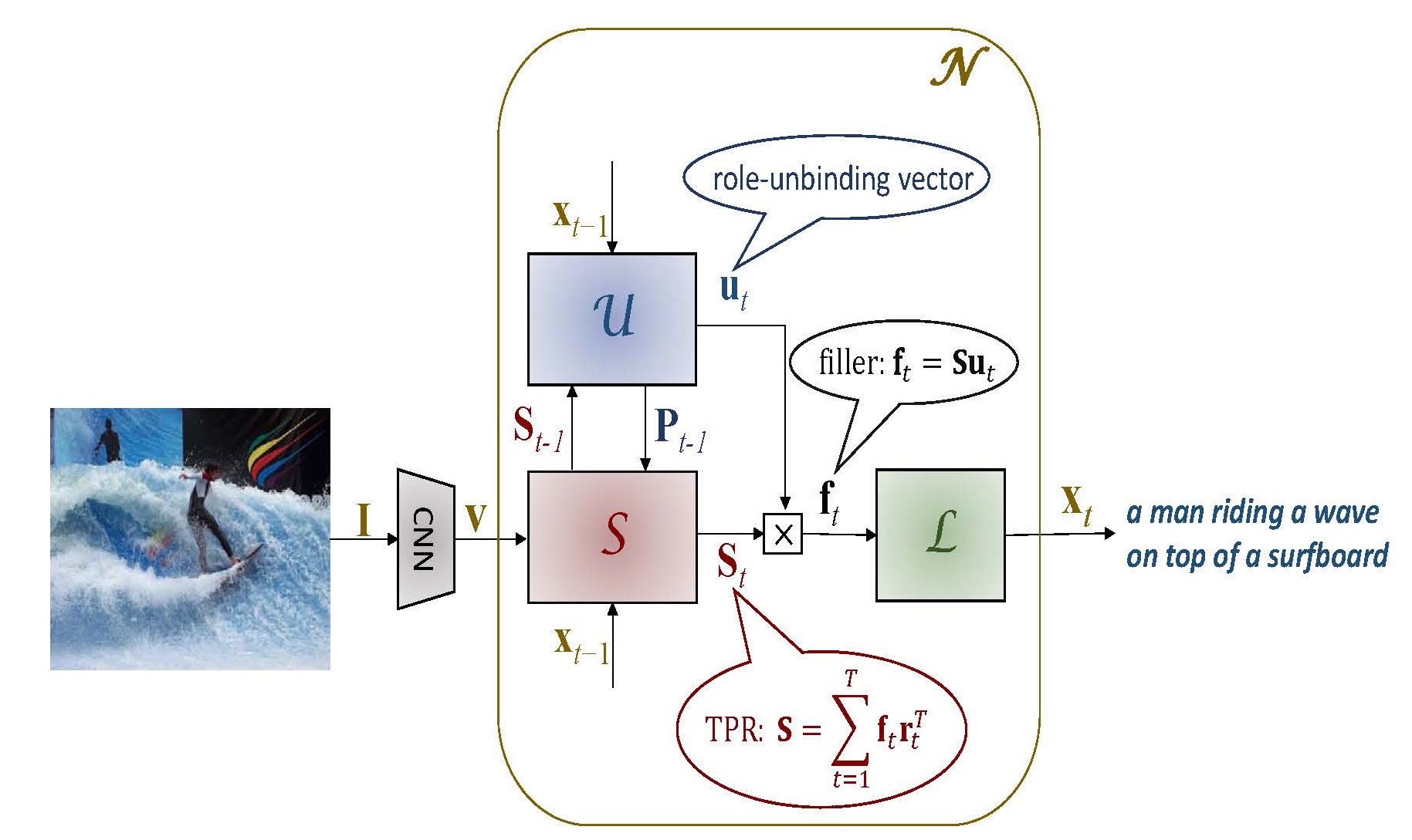
Figure 1: Architecture of TPGN, a TPR-capable generation network. “$\Box\times$” denotes the matrix-vector product.

3 A TPR-capable generation architecture

As Fig. 1 shows, the proposed Tensor Product Generation Network architecture (the dashed box labeled $\mathcal{N}$) is designed to support the technique for generation just described: the architecture is TPR-capable. There is a sentence-encoding subnetwork $\mathcal{S}$ which could host a TPR of the sentence to be generated, and an unbinding subnetwork $\mathcal{U}$ which could output a sequence of unbinding vectors $\mathbf{u}_{t}$; at time $t$, the embedding $\mathbf{f}_{t}$ of the word produced, $\texttt{x}_{t}$, could then be extracted from $\mathbf{S}_{t}$ via the matrix-vector product (shown in the figure by “$\Box\times$”): $\mathbf{f}_{t}=\mathbf{S}_{t}\mathbf{u}_{t}$. The lexical-decoding subnetwork $\mathcal{L}$ converts the embedding vector $\mathbf{f}_{t}$ to the 1-hot vector $\mathbf{x}_{t}$ corresponding to the word $\texttt{x}_{t}$.

Unlike some other work [23], TPGN is not constrained to literally learn TPRs. The representations that will actually be housed in $\mathcal{S}$ and $\mathcal{U}$ are determined by end-to-end deep learning on a task: the bubbles in Fig. 1 show what would be the meanings of $\mathbf{S}_{t},\mathbf{u}_{t}$ and $\mathbf{f_{t}}$ if an actual TPR scheme were instantiated in the architecture. The learned representations $\mathbf{S}_{t}$ will not be proven to literally be TPRs, but by analyzing the unbinding vectors $\mathbf{u}_{t}$ the network learns, we will gain insight into the process by which the learned matrices $\mathbf{S}_{t}$ give rise to the generated sentence.

The task studied here is image captioning; Fig. 1 shows that the input to this TPGN model is an image, preprocessed by a CNN which produces the initial representation in $\mathcal{S}$, $\mathbf{S}_{0}$. This vector $\mathbf{S}_{0}$ drives the entire caption-generation process: it contains all the image-specific information for producing the caption. (We will call a caption a “sentence” even though it may in fact be just a noun phrase.)

The two subnets $\mathcal{S}$ and $\mathcal{U}$ are mutually-connected LSTMs [13]: see Fig. 2. The internal hidden state of $\mathcal{U}$, $\mathbf{p}_{t}$, is sent as input to $\mathcal{S}$; $\mathcal{U}$ also produces output, the unbinding vector $\mathbf{u}_{t}$. The internal hidden state of $\mathcal{S}$, $\mathbf{S}_{t}$, is sent as input to $\mathcal{U}$, and also produced as output. As stated above, these two outputs are multiplied together to produce the embedding vector $\mathbf{f}_{t}=\mathbf{S}_{t}\mathbf{u}_{t}$ of the output word $\texttt{x}_{t}$. Furthermore, the 1-hot encoding $\mathbf{x}_{t}$ of $\texttt{x}_{t}$ is fed back at the next time step to serve as input to both $\mathcal{S}$ and $\mathcal{U}$.

What type of roles might the unbinding vectors be unbinding? A TPR for a caption could in principle be built upon positional roles, syntactic/semantic roles, or some combination of the two. In the caption a man standing in a room with a suitcase, the initial a and man might respectively occupy the positional roles of $\textsc{pos(ition)}_{1}$ and $\textsc{pos}_{2}$; standing might occupy the syntactic role of verb; in the role of Spatial-P(reposition); while a room with a suitcase might fill a 5-role schema $\textsc{Det(erminer)}_{1}\textsc{ N(oun)}_{1}\textsc{ P Det}_{2}\textsc{ N}_{2}$. In fact we will provide evidence in Sec. 5.3.2 that our network learns just this kind of hybrid role decomposition; further evidence for these particular roles is presented elsewhere.

What form of information does the sentence-encoding subnetwork $\mathcal{S}$ need to encode in $\mathbf{S}$? Continuing with the example of the previous paragraph, $\mathbf{S}$ needs to be some approximation to the TPR summing several filler/role binding matrices. In one of these bindings, a filler vector $\mathbf{f}_{\texttt{a}}$ — which the lexical subnetwork $\mathcal{L}$ will map to the article a — is bound (via the outer product) to a role vector $\mathbf{r}_{\textsc{Pos}_{1}}$ which is the dual of the first unbinding vector produced by the unbinding subnetwork $\mathcal{U}$: $\mathbf{u}_{\textsc{Pos}_{1}}$. In the first iteration of generation the model computes $\mathbf{S}_{1}\mathbf{u}_{\textsc{Pos}_{1}}=\mathbf{f}_{\texttt{a}}$, which $\mathcal{L}$ then maps to a. Analogously, another binding approximately contained in $\mathbf{S}_{2}$ is $\mathbf{f}_{\texttt{man}}\mathbf{r}_{\textsc{Pos}_{2}}^{\top}$. There are corresponding approximate bindings for the remaining words of the caption; these employ syntactic/semantic roles. One example is $\mathbf{f}_{\texttt{standing}}\mathbf{r}_{V}^{\top}$. At iteration 3, $\mathcal{U}$ decides the next word should be a verb, so it generates the unbinding vector $\mathbf{u}_{V}$ which when multiplied by the current output of $\mathcal{S}$, the matrix $\mathbf{S}_{3}$, yields a filler vector $\mathbf{f}_{\texttt{standing}}$ which $\mathcal{L}$ maps to the output standing. $\mathcal{S}$ decided the caption should deploy standing as a verb and included in $\mathbf{S}$ an approximation to the binding $\mathbf{f}_{\texttt{standing}}\mathbf{r}_{V}^{\top}$. It similarly decided the caption should deploy in as a spatial preposition, approximately including in $\mathbf{S}$ the binding $\mathbf{f}_{\texttt{in}}\mathbf{r}_{\textsc{Spatial-P}}^{\top}$; and so on for the other words in their respective roles in the caption.

4 System Description

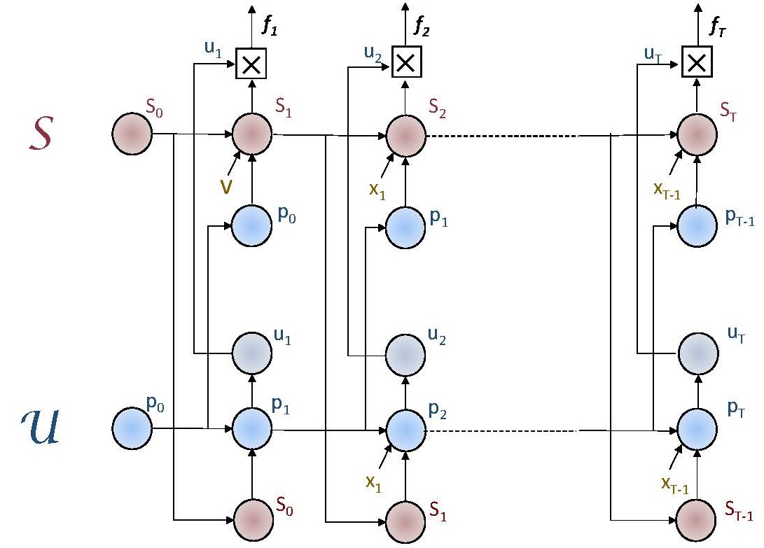
Figure 2: The sentence-encoding subnet $\mathcal{S}$ and the unbinding subnet $\mathcal{U}$ are inter-connected LSTMs; $\mathbf{v}$ encodes the visual input while the $\mathbf{x}_{t}$ encode the words of the output caption.

As stated above, the unbinding subnetwork $\mathcal{U}$ and the sentence-encoding subnetwork $\mathcal{S}$ of Fig. 1 are each implemented as (1-layer, 1-directional) LSTMs (see Fig. 2); the lexical subnetwork $\mathcal{L}$ is implemented as a linear transformation followed by a softmax operation.

In the equations below, the LSTM variables internal to the $\mathcal{S}$ subnet are indexed by 1 (e.g., the forget-, input-, and output-gates are respectively $\mathbf{\hat{f}}_{1},\mathbf{\hat{i}}_{1},\mathbf{\hat{o}}_{1}$) while those of the unbinding subnet $\mathcal{U}$ are indexed by 2.

Thus the state updating equations for $\mathcal{S}$ are, for $t=1,\cdots,T$ = caption length:

$${\mathbf{\hat{f}}}_{1,t}=\sigma_{g}({\mathbf{W}}_{1,f}{\mathbf{p}}_{t-1}-{\mathbf{D}}_{1,f}{\mathbf{W}}_{e}{\mathbf{x}}_{t-1}+{\mathbf{U}}_{1,f}{\mathbf{\hat{S}}}_{t-1})$$ (3)

$${\mathbf{\hat{i}}}_{1,t}=\sigma_{g}({\mathbf{W}}_{1,i}{\mathbf{p}}_{t-1}-{\mathbf{D}}_{1,i}{\mathbf{W}}_{e}{\mathbf{x}}_{t-1}+{\mathbf{U}}_{1,i}{\mathbf{\hat{S}}}_{t-1})$$ (4)

$${\mathbf{\hat{o}}}_{1,t}=\sigma_{g}({\mathbf{W}}_{1,o}{\mathbf{p}}_{t-1}-{\mathbf{D}}_{1,o}{\mathbf{W}}_{e}{\mathbf{x}}_{t-1}+{\mathbf{U}}_{1,o}{\mathbf{\hat{S}}}_{t-1})$$ (5)

$${\mathbf{g}}_{1,t}=\sigma_{h}({\mathbf{W}}_{1,c}{\mathbf{p}}_{t-1}-{\mathbf{D}}_{1,c}{\mathbf{W}}_{e}{\mathbf{x}}_{t-1}+{\mathbf{U}}_{1,c}{\mathbf{\hat{S}}}_{t-1})$$ (6)

$${\mathbf{c}}_{1,t}={\mathbf{\hat{f}}}_{1,t}\odot{\mathbf{c}}_{1,t-1}+{\mathbf{\hat{i}}}_{1,t}\odot{\mathbf{g}}_{1,t}\quad\quad\quad$$ (7)

$${\mathbf{\hat{S}}}_{t}={\mathbf{\hat{o}}}_{1,t}\odot\sigma_{h}({\mathbf{c}}_{1,t})\quad\quad\quad\quad\quad\quad\quad$$ (8)

Here ${\mathbf{\hat{f}}}_{1,t}$, ${\mathbf{\hat{i}}}_{1,t}$, ${\mathbf{\hat{o}}}_{1,t}$, ${\mathbf{g}}_{1,t}$, ${\mathbf{c}}_{1,t}$, ${\mathbf{\hat{S}}}_{t}\in\mathbb{R}^{d\times d}$, ${\mathbf{p}}_{t}\in\mathbb{R}^{d}$; $\sigma_{g}(\cdot)$ is the (element-wise) logistic sigmoid function; $\sigma_{h}(\cdot)$ is the hyperbolic tangent function; the operator $\odot$ denotes the Hadamard (element-wise) product; ${\mathbf{W}}_{1,f},{\mathbf{W}}_{1,i},{\mathbf{W}}_{1,o},{\mathbf{W}}_{1,c}\in\mathbb{R}^{d\times d\times d}$, ${\mathbf{D}}_{1,f}$, ${\mathbf{D}}_{1,i}$, ${\mathbf{D}}_{1,o}$, ${\mathbf{D}}_{1,c}$ $\in$ $\mathbb{R}^{d\times d\times d}$, ${\mathbf{U}}_{1,f}$, ${\mathbf{U}}_{1,i}$, ${\mathbf{U}}_{1,o}$, ${\mathbf{U}}_{1,c}$ $\in$ $\mathbb{R}^{d\times d\times d\times d}$. For clarity, biases — included throughout the model — are omitted from all equations in this paper. The initial state ${\mathbf{\hat{S}}}_{0}$ is initialized by:

$${\mathbf{\hat{S}}}_{0}={\mathbf{C}}_{s}({\mathbf{v}}-\bar{{\mathbf{v}}})$$ (9)

where ${\mathbf{v}}\in\mathbb{R}^{2048}$ is the vector of visual features extracted from the current image by ResNet [10] and $\bar{{\mathbf{v}}}$ is the mean of all such vectors; ${\mathbf{C}}_{s}\in\mathbb{R}^{d\times d\times 2048}$. On the output side, ${\mathbf{x}}_{t}\in\mathbb{R}^{V}$ is a 1-hot vector with dimension equal to the size of the caption vocabulary, $V$, and ${\mathbf{W}}_{e}\in\mathbb{R}^{d\times V}$ is a word embedding matrix, the $i$-th column of which is the embedding vector of the $i$-th word in the vocabulary; it is obtained by the Stanford GLoVe algorithm with zero mean [25]. ${\mathbf{x}}_{0}$ is initialized as the one-hot vector corresponding to a “start-of-sentence” symbol.

For $\mathcal{U}$ in Fig. 1, the state updating equations are:

$${\mathbf{\hat{f}}}_{2,t}=\sigma_{g}({\mathbf{\hat{S}}}_{t-1}{\mathbf{w}}_{2,f}-{\mathbf{D}}_{2,f}{\mathbf{W}}_{e}{\mathbf{x}}_{t-1}+{\mathbf{U}}_{2,f}{\mathbf{p}}_{t-1})$$ (10)

$${\mathbf{\hat{i}}}_{2,t}=\sigma_{g}({\mathbf{\hat{S}}}_{t-1}{\mathbf{w}}_{2,i}-{\mathbf{D}}_{2,i}{\mathbf{W}}_{e}{\mathbf{x}}_{t-1}+{\mathbf{U}}_{2,i}{\mathbf{p}}_{t-1})$$ (11)

$${\mathbf{\hat{o}}}_{2,t}=\sigma_{g}({\mathbf{\hat{S}}}_{t-1}{\mathbf{w}}_{2,o}-{\mathbf{D}}_{2,o}{\mathbf{W}}_{e}{\mathbf{x}}_{t-1}+{\mathbf{U}}_{2,o}{\mathbf{p}}_{t-1})$$ (12)

$${\mathbf{g}}_{2,t}=\sigma_{h}({\mathbf{\hat{S}}}_{t-1}{\mathbf{w}}_{2,c}-{\mathbf{D}}_{2,c}{\mathbf{W}}_{e}{\mathbf{x}}_{t-1}+{\mathbf{U}}_{2,c}{\mathbf{p}}_{t-1})$$ (13)

$${\mathbf{c}}_{2,t}={\mathbf{\hat{f}}}_{2,t}\odot{\mathbf{c}}_{2,t-1}+{\mathbf{\hat{i}}}_{2,t}\odot{\mathbf{g}}_{2,t}\quad\quad\quad$$ (14)

$${\mathbf{p}}_{t}={\mathbf{\hat{o}}}_{2,t}\odot\sigma_{h}({\mathbf{c}}_{2,t})\quad\quad\quad\quad\quad\quad\quad$$ (15)

Here ${\mathbf{w}}_{2,f},{\mathbf{w}}_{2,i},{\mathbf{w}}_{2,o},{\mathbf{w}}_{2,c}\in\mathbb{R}^{d}$, ${\mathbf{D}}_{2,f}$, ${\mathbf{D}}_{2,i}$, ${\mathbf{D}}_{2,o}$, ${\mathbf{D}}_{2,c}$ $\in$ $\mathbb{R}^{d\times d}$, and ${\mathbf{U}}_{2,f}$, ${\mathbf{U}}_{2,i}$, ${\mathbf{U}}_{2,o}$, ${\mathbf{U}}_{2,c}$ $\in$ $\mathbb{R}^{d\times d}$. The initial state ${\mathbf{p}}_{0}$ is the zero vector.

The dimensionality of the crucial vectors shown in Fig. 1, $\mathbf{u}_{t}$ and $\mathbf{f}_{t}$, is increased from $d\times 1$ to $d^{2}\times 1$ as follows. A block-diagonal $d^{2}\times d^{2}$ matrix $\mathbf{S}_{t}$ is created by placing $d$ copies of the $d\times d$ matrix $\mathbf{\hat{S}}_{t}$ as blocks along the principal diagonal. This matrix is the output of the sentence-encoding subnetwork $\mathcal{S}$. Now the ‘filler vector’ ${\mathbf{f}}_{t}\in\mathbb{R}^{d^{2}}$ — ‘unbound’ from the sentence representation $\mathbf{S}_{t}$ with the ‘unbinding vector’ $\mathbf{u}_{t}$ — is obtained by Eq. (16).

$${\mathbf{f}}_{t}={\mathbf{S}}_{t}{\mathbf{u}}_{t}$$ (16)

Here ${\mathbf{u}}_{t}\in\mathbb{R}^{d^{2}}$, the output of the unbinding subnetwork $\mathcal{U}$, is computed as in Eq. (17), where ${\mathbf{W}}_{u}\in\mathbb{R}^{d^{2}\times d}$ is $\mathcal{U}$’s output weight matrix.

$${\mathbf{u}}_{t}=\sigma_{h}({\mathbf{W}}_{u}{\mathbf{p}}_{t})$$ (17)

Finally, the lexical subnetwork $\mathcal{L}$ produces a decoded word ${\mathbf{x}}_{t}\in\mathbb{R}^{V}$ by

$${\mathbf{x}}_{t}=\sigma_{s}({\mathbf{W}}_{x}{\mathbf{f}}_{t})$$ (18)

where $\sigma_{s}(\cdot)$ is the softmax function and ${\mathbf{W}}_{x}\in\mathbb{R}^{V\times d^{2}}$ is the overall output weight matrix. Since ${\mathbf{W}}_{x}$ plays the role of a word de-embedding matrix, we can set

$${\mathbf{W}}_{x}=({\mathbf{W}}_{e})^{\top}$$ (19)

where ${\mathbf{W}}_{e}$ is the word-embedding matrix. Since ${\mathbf{W}}_{e}$ is pre-defined, we directly set ${\mathbf{W}}_{x}$ by Eq. (19) without training $\mathcal{L}$ through Eq. (18). Note that $\mathcal{S}$ and $\mathcal{U}$ are learned jointly through the end-to-end training as shown in Algorithm 1.

Algorithm 1 End-to-end training of $\mathcal{S}$ and $\mathcal{U}$

Input: Image feature vector ${\mathbf{v}}^{(i)}$ and corresponding caption ${\mathbf{X}}^{(i)}=[{\mathbf{x}}_{1}^{(i)}$, $\cdots$, ${\mathbf{x}}_{T}^{(i)}]$ ($i=1$ , $\cdots$, $N$), where $N$ is the total number of samples.
Output: ${\mathbf{W}}_{1,f},{\mathbf{W}}_{1,i},{\mathbf{W}}_{1,o},{\mathbf{W}}_{1,c},{\mathbf{C}}_{s},{\mathbf{D}}_{1,f},{\mathbf{D}}_{1,i},{\mathbf{D}}_{1,o}$,
${\mathbf{D}}_{1,c},{\mathbf{U}}_{1,f},{\mathbf{U}}_{1,i},{\mathbf{U}}_{1,o},{\mathbf{U}}_{1,c},{\mathbf{w}}_{2,f},{\mathbf{w}}_{2,i},{\mathbf{w}}_{2,o},{\mathbf{w}}_{2,c},{\mathbf{D}}_{2,f}$,
${\mathbf{D}}_{2,i},{\mathbf{D}}_{2,o},{\mathbf{D}}_{2,c},{\mathbf{U}}_{2,f},{\mathbf{U}}_{2,i},{\mathbf{U}}_{2,o},{\mathbf{U}}_{2,c},{\mathbf{W}}_{u},{\mathbf{W}}_{x}$.

1:  Initialize ${\mathbf{S}}_{0}$ by (9);

2:  Initialize ${\mathbf{x}}_{0}$ as the one-hot vector corresponding to the start-of-sentence symbol;

3:  Initialize ${\mathbf{p}}_{0}$ as the zero vector;

4:  Randomly initialize weights ${\mathbf{W}}_{1,f},{\mathbf{W}}_{1,i},{\mathbf{W}}_{1,o}$,${\mathbf{W}}_{1,c},{\mathbf{C}}_{s},{\mathbf{D}}_{1,f},{\mathbf{D}}_{1,i},{\mathbf{D}}_{1,o},{\mathbf{D}}_{1,c},{\mathbf{U}}_{1,f},{\mathbf{U}}_{1,i},{\mathbf{U}}_{1,o}$,${\mathbf{U}}_{1,c},{\mathbf{w}}_{2,f},{\mathbf{w}}_{2,i},{\mathbf{w}}_{2,o},{\mathbf{w}}_{2,c},{\mathbf{D}}_{2,f},{\mathbf{D}}_{2,i},{\mathbf{D}}_{2,o}$,${\mathbf{D}}_{2,c},{\mathbf{U}}_{2,f},{\mathbf{U}}_{2,i},{\mathbf{U}}_{2,o},{\mathbf{U}}_{2,c},{\mathbf{W}}_{u},{\mathbf{W}}_{x}$;

5:  for $n$ from $1$ to $N$ do

6:     for $t$ from $1$ to $T$ do

7:        Calculate (3) – (8) to obtain ${\mathbf{S}}_{t}$;

8:        Calculate (10) – (15) to obtain ${\mathbf{p}}_{t}$;

9:        Calculate (17) to obtain ${\mathbf{u}}_{t}$;

10:        Calculate (16) to obtain ${\mathbf{f}}_{t}$;

11:        Calculate (18) to obtain ${\mathbf{x}}_{t}$;

12:        Update weights ${\mathbf{W}}_{1,f},{\mathbf{W}}_{1,i},{\mathbf{W}}_{1,o}$,${\mathbf{W}}_{1,c},{\mathbf{C}}_{s},{\mathbf{D}}_{1,f},{\mathbf{D}}_{1,i},{\mathbf{D}}_{1,o},{\mathbf{D}}_{1,c},{\mathbf{U}}_{1,f},{\mathbf{U}}_{1,i}$,${\mathbf{U}}_{1,o},{\mathbf{U}}_{1,c},{\mathbf{w}}_{2,f},{\mathbf{w}}_{2,i},{\mathbf{w}}_{2,o},{\mathbf{w}}_{2,c},{\mathbf{D}}_{2,f},{\mathbf{D}}_{2,i}$,${\mathbf{D}}_{2,o},{\mathbf{D}}_{2,c},{\mathbf{U}}_{2,f},{\mathbf{U}}_{2,i},{\mathbf{U}}_{2,o},{\mathbf{U}}_{2,c},{\mathbf{W}}_{u},{\mathbf{W}}_{x}$ by the back-propagation algorithm;

13:     end for

14:  end for

5 Experimental results

5.1 Dataset

To evaluate the performance of our proposed model, we use the COCO dataset [6]. The COCO dataset contains 123,287 images, each of which is annotated with at least 5 captions. We use the same pre-defined splits as in [14, 10]: 113,287 images for training, 5,000 images for validation, and 5,000 images for testing. We use the same vocabulary as that employed in [10], which consists of 8,791 words.

5.2 Evaluation

For the CNN of Fig. 1, we used ResNet-152 [12], pretrained on the ImageNet dataset. The feature vector ${\mathbf{v}}$ has 2048 dimensions. Word embedding vectors in ${\mathbf{W}}_{e}$ are downloaded from the web [25]. The model is implemented in TensorFlow [1] with the default settings for random initialization and optimization by backpropagation.

In our experiments, we choose $d=25$ (where $d$ is the dimension of vector ${\mathbf{p}}_{t}$). The dimension of ${\mathbf{S}}_{t}$ is $625\times 625$ (while $\mathbf{\hat{S}}_{t}$ is $25\times 25$); the vocabulary size $V=8,791$; the dimension of ${\mathbf{u}}_{t}$ and ${\mathbf{f}}_{t}$ is $d^{2}=625$.

Table 1: Performance of the proposed TPGN model on the COCO dataset.

Methods	METEOR	BLEU-1	BLEU-2	BLEU-3	BLEU-4	CIDEr
NIC [33]	0.237	0.666	0.461	0.329	0.246	0.855
CNN-LSTM	0.238	0.698	0.525	0.390	0.292	0.889
TPGN	0.243	0.709	0.539	0.406	0.305	0.909

The main evaluation results on the MS COCO dataset are reported in Table 1. The widely-used BLEU [24], METEOR [3], and CIDEr [32] metrics are reported in our quantitative evaluation of the performance of the proposed model. In evaluation, our baseline is the widely used CNN-LSTM captioning method originally proposed in [33]. For comparison, we include results in that paper in the first line of Table 1. We also re-implemented the model using the latest ResNet features and report the results in the second line of Table 1. Our re-implementation of the CNN-LSTM method matches the performance reported in [10], showing that the baseline is a state-of-the-art implementation. As shown in Table 1, compared to the CNN-LSTM baseline, the proposed TPGN significantly outperforms the benchmark schemes in all metrics across the board. The improvement in BLEU-$n$ is greater for greater $n$; TPGN particularly improves generation of longer subsequences. The results attest to the effectiveness of the TPGN architecture.

5.3 Interpretation of learned unbinding vectors

To get a sense of how the sentence encodings $\mathbf{S}_{t}$ learned by TPGN approximate TPRs, we now investigate the meaning of the role-unbinding vector $\mathbf{u}_{t}$ the model uses to unbind from $\mathbf{S}_{t}$ — via Eq. (16) — the filler vector $\mathbf{f}_{t}$ that produces — via Eq. (18) — the one-hot vector $\mathbf{x}_{t}$ of the $t^{\textrm{th}}$ generated caption word. The meaning of an unbinding vector is the meaning of the role it unbinds. Interpreting the unbinding vectors reveals the meaning of the roles in a TPR that $\mathbf{S}$ approximates.

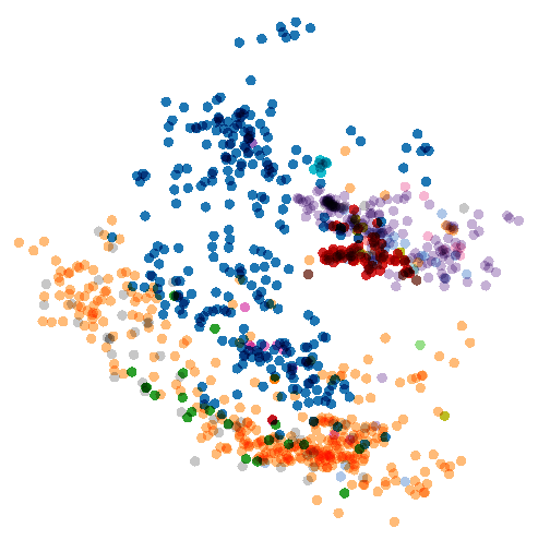
Figure 3: Unbinding vectors of 1000 words; different POS tags of words are represented by different colors.

5.3.1 Visualization of ${\mathbf{u}}_{t}$

We run the TPGN model with 5,000 test images as input, and obtain the unbinding vector ${\mathbf{u}}_{t}$ used to generate each word ${\mathbf{x}}_{t}$ in the caption of a test image. We plot 1,000 unbinding vectors ${\mathbf{u}}_{t}$, which correspond to the first 1,000 words in the resulting captions of these 5,000 test images. There are 17 parts of speech (POS) in these 1,000 words. The POS tags are obtained by the Stanford Parser [20].

We use the Embedding Projector in TensorBoard [11] to plot 1,000 unbinding vectors ${\mathbf{u}}_{t}$ with a custom linear projection in TensorBoard to reduce 625 dimensions of ${\mathbf{u}}_{t}$ to 2 dimensions shown in Fig. 3 through Fig. 7.

Fig. 3 shows the unbinding vectors of 1000 words; different POS tags of words are represented by different colors. In fact, we can partition the 625-dim space of ${\mathbf{u}}_{t}$ into 17 regions, each of which contains 76.3% words of the same type of POS on average; i.e., each region is dominated by words of one POS type. This clearly indicates that each unbinding vector contains important grammatical information about the word it generates. As examples, Fig. 4 to Fig. 7 show the distribution of the unbinding vectors of nouns, verbs, adjectives, and prepositions, respectively.

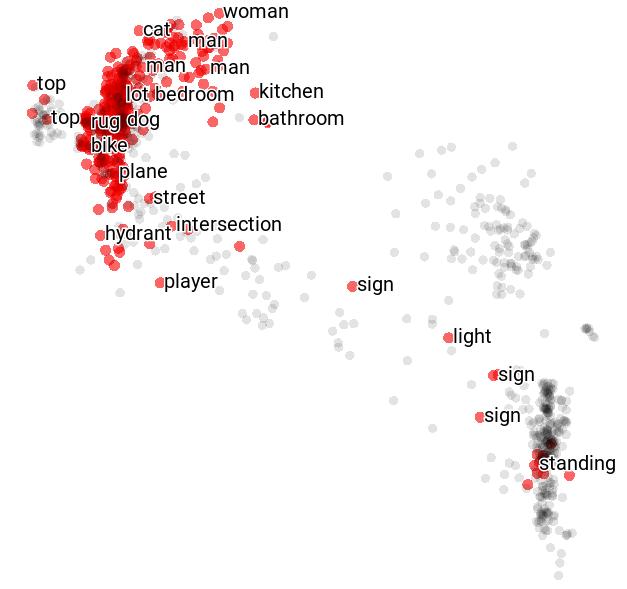
Figure 4: Unbinding vectors of 360 nouns in red and 640 words of other types of POS in grey.

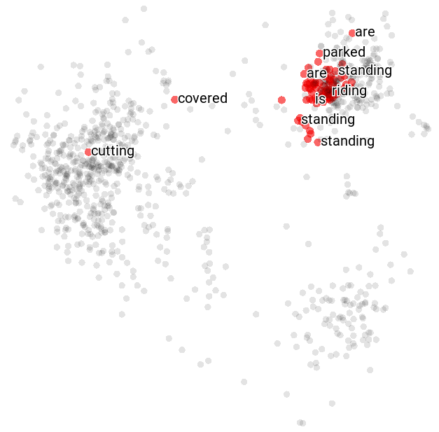
Figure 5: Unbinding vectors of 81 verbs in red and 919 words of other types of POS in grey.

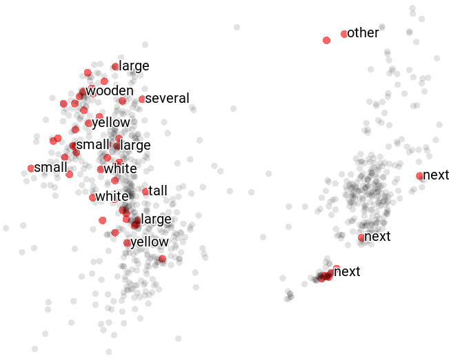
Figure 6: Unbinding vectors of 55 adjectives in red and 945 words of other types of POS in grey.

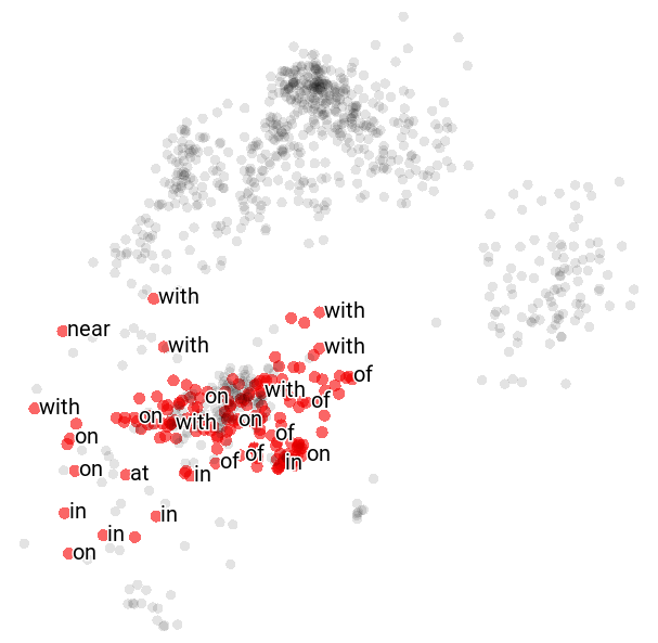
Figure 7: Unbinding vectors of 169 prepositions in red and 831 words of other types of POS in grey.

Table 2: Conformity to N/V generalization ($N_{u}=2)$.

Category	$N_{w}$	$N_{r}$	$P_{c}$
Nouns	16683	16115	0.969
Pronouns	462	442	0.957
Indefinite articles	7248	7107	0.981
Definite articles	797	762	0.956
Adjectives	2543	2237	0.880
Verbs	3558	3409	0.958
Prepositions & conjunctions	8184	7859	0.960
Adverbs	13	8	0.615

Table 3: Interpretation of unbinding clusters ($N_{u}=10)$

ID	Interpretation (proportion)
2	Position 1 (1.00)
3	Position 2 (1.00)
1	Noun (0.54), Determiner (0.43)
5	Determiner (0.50), Noun (0.19), Preposition (0.15)
7	Noun (0.88), Adjective (0.09)
9	Determiner (0.90), Noun (0.10)
0	Preposition (0.64), . (0.16), V (0.14)
4	Preposition: spatial (0.72) non-spatial (0.19)
6	Preposition (0.59), . (0.14)
8	Verb (0.37), Preposition (0.36), . (0.20)

5.3.2 Clustering of ${\mathbf{u}}_{t}$

Since the previous section indicates that there is a clustering structure for ${\mathbf{u}}_{t}$, in this section we partition ${\mathbf{u}}_{t}$ into $N_{u}$ clusters and examine the grammar roles played by ${\mathbf{u}}_{t}$ .

First, we run the trained TPGN model on the 113,287 training images, obtaining the role-unbinding vector ${\mathbf{u}}_{t}$ used to generate each word ${\mathbf{x}}_{t}$ in the caption sentence. There are approximately 1.2 million ${\mathbf{u}}_{t}$ vectors over all the training images. We apply the K-means clustering algorithm to these vectors to obtain $N_{u}$ clusters and the centroid ${\bm{\mu}}_{i}$ of each cluster $i$ ($i=0,\cdots,N_{u}-1$).

Then, we run the TPGN model with 5,000 test images as input, and obtain the role vector ${\mathbf{u}}_{t}$ of each word ${\mathbf{x}}_{t}$ in the caption sentence of a test image. Using the nearest neighbor rule, we obtain the index $i$ of the cluster that each ${\mathbf{u}}_{t}$ is assigned to.

The partitioning of the unbinding vectors ${\mathbf{u}}_{t}$ into $N_{u}=2$ clusters exposes the most fundamental distinction made by the roles. We find that the vectors assigned to Cluster 1 generate words which are nouns, pronouns, indefinite and definite articles, and adjectives, while the vectors assigned to Cluster 0 generate verbs, prepositions, conjunctions, and adverbs. Thus Cluster 1 contains the noun-related words, Cluster 0 the verb-like words (verbs, prepositions and conjunctions are all potentially followed by noun-phrase complements, for example). Cross-cutting this distinction is another dimension, however: the initial word in a caption (always a determiner) is sometimes generated with a Cluster 1 unbinding vector, sometimes with a Cluster 0 vector. Outside the caption-initial position, exceptions to the nominal/verbal $\sim$ Cluster 1/0 generalization are rare, as attested by the high rates of conformity to the generalization shown in Table 2 .

Table 2 shows the likelihood of correctness of this ‘N/V’ generalization for the words in 5,000 sentences captioned for the 5,000 test images; $N_{w}$ is the number of words in the category, $N_{r}$ is the number of words conforming to the generalization, and $P_{c}=N_{r}/N_{w}$ is the proportion conforming. We use the Natural Language Toolkit [22] to identify the part of speech of each word in the captions.

A similar analysis with $N_{u}=10$ clusters reveals the results shown in Table 3; these results concern the first 100 captions, which were inspected manually to identify interpretable patterns. (More comprehensive results will be discussed elsewhere.)

The clusters can be interpreted as falling into 3 groups (see Table 3). Clusters 2 and 3 are clearly positional roles: every initial word is generated by a role-unbinding vector from Cluster 2, and such vectors are not used elsewhere in the string. The same holds for Cluster 3 and the second caption word.

For caption words after the second word, position is replaced by syntactic/semantic properties for interpretation purposes. The vector clusters aside from 2 and 3 generate words with a dominant grammatical category: for example, unbinding vectors assigned to the cluster 4 generate words that are 91% likely to be prepositions, and 72% likely to be spatial prepositions. Cluster 7 generates 88% nouns and 9% adjectives, with the remaining 3% scattered across other categories. As Table 3 shows, clusters 1, 5, 7, 9 are primarily nominal, and 0, 4, 6, and 8 primarily verbal. (Only cluster 5 spans the N/V divide.)

6 Related work

This work follows a great deal of recent caption-generation literature in exploiting end-to-end deep learning with a CNN image-analysis front end producing a distributed representation that is then used to drive a natural-language generation process, typically using RNNs [21, 33, 7, 4, 8, 14, 15, 16]. Our grammatical interpretation of the structural roles of words in sentences makes contact with other work that incorporates deep learning into grammatically-structured networks [31, 18, 17, 2, 34, 19, 30, 26]. Here, the network is not itself structured to match the grammatical structure of sentences being processed; the structure is fixed, but is designed to support the learning of distributed representations that incorporate structure internal to the representations themselves — filler/role structure.

TPRs are also used in NLP in [23] but there the representation of each individual input word is constrained to be a literal TPR filler/role binding. (The idea of using the outer product to construct internal representations was also explored in [9].) Here, by contrast, the learned representations are not themselves constrained, but the global structure of the network is designed to display the somewhat abstract property of being TPR-capable: the architecture uses the TPR unbinding operation of the matrix-vector product to extract individual words for sequential output.

7 Conclusion

Tensor Product Representation (TPR) [27] is a general technique for constructing vector embeddings of complex symbol structures in such a way that powerful symbolic functions can be computed using hand-designed neural network computation. Integrating TPR with deep learning is a largely open problem for which the work presented here proposes a general approach: design deep architectures that are TPR-capable — TPR computation is within the scope of the capabilities of the architecture in principle. For natural language generation, we proposed such an architecture, the Tensor Product Generation Network (TPGN): it embodies the TPR operation of unbinding which is used to extract particular symbols (e.g., words) from complex structures (e.g., sentences). The architecture can be interpreted as containing a part that encodes a sentence and a part that selects one structural role at a time to extract from the sentence. We applied the approach to image-caption generation, developing a TPGN model that was evaluated on the COCO dataset, on which it outperformed LSTM baselines on a range of standard metrics. Unlike standard LSTMs, however, the TPGN model admits a level of interpretability: we can see which roles are being unbound by the unbinding vectors generated internally within the model. We find such roles contain considerable grammatical information, enabling POS tag prediction for the words they generate and displaying clustering by POS.

References

- [1] Martín Abadi, Ashish Agarwal, Paul Barham, Eugene Brevdo, Zhifeng Chen, Craig Citro, Greg S. Corrado, Andy Davis, Jeffrey Dean, Matthieu Devin, Sanjay Ghemawat, Ian Goodfellow, Andrew Harp, Geoffrey Irving, Michael Isard, Yangqing Jia, Rafal Jozefowicz, Lukasz Kaiser, Manjunath Kudlur, Josh Levenberg, Dan Mané, Rajat Monga, Sherry Moore, Derek Murray, Chris Olah, Mike Schuster, Jonathon Shlens, Benoit Steiner, Ilya Sutskever, Kunal Talwar, Paul Tucker, Vincent Vanhoucke, Vijay Vasudevan, Fernanda Viégas, Oriol Vinyals, Pete Warden, Martin Wattenberg, Martin Wicke, Yuan Yu, and Xiaoqiang Zheng. TensorFlow: Large-scale machine learning on heterogeneous systems, 2015. Software available from tensorflow.org.
- [2] Jacob Andreas, Marcus Rohrbach, Trevor Darrell, and Dan Klein. Deep compositional question answering with neural module networks. arxiv preprint. arXiv preprint arXiv:1511.02799, 2, 2015.
- [3] Satanjeev Banerjee and Alon Lavie. Meteor: An automatic metric for mt evaluation with improved correlation with human judgments. In Proceedings of the ACL workshop on intrinsic and extrinsic evaluation measures for machine translation and/or summarization, pages 65–72. Association for Computational Linguistics, 2005.
- [4] Xinlei Chen and Lawrence Zitnick. Mind’s eye: A recurrent visual representation for image caption generation. In Proceedings of the IEEE Conference on Computer Vision and Pattern Recognition, pages 2422–2431, 2015.
- [5] Pyeong Whan Cho, Matthew Goldrick, and Paul Smolensky. Incremental parsing in a continuous dynamical system: Sentence processing in Gradient Symbolic Computation. Linguistics Vanguard, 3, 2017.
- [6] COCO. Coco dataset for image captioning. http://mscoco.org/dataset/#download, 2017.
- [7] Jacob Devlin, Hao Cheng, Hao Fang, Saurabh Gupta, Li Deng, Xiaodong He, Geoffrey Zweig, and Margaret Mitchell. Language models for image captioning: The quirks and what works. arXiv preprint arXiv:1505.01809, 2015.
- [8] Jeffrey Donahue, Lisa Anne Hendricks, Sergio Guadarrama, Marcus Rohrbach, Subhashini Venugopalan, Kate Saenko, and Trevor Darrell. Long-term recurrent convolutional networks for visual recognition and description. In Proceedings of the IEEE conference on computer vision and pattern recognition, pages 2625–2634, 2015.
- [9] Akira Fukui, Dong Huk Park, Daylen Yang, Anna Rohrbach, Trevor Darrell, and Marcus Rohrbach. Multimodal compact bilinear pooling for visual question answering and visual grounding. arXiv preprint arXiv:1606.01847, 2016.
- [10] Zhe Gan, Chuang Gan, Xiaodong He, Yunchen Pu, Kenneth Tran, Jianfeng Gao, Lawrence Carin, and Li Deng. Semantic compositional networks for visual captioning. In Proceedings of the IEEE Conference on Computer Vision and Pattern Recognition, 2017.
- [11] Google. Embedding projector in tensorboard. https://www.tensorflow.org/programmers_guide/embedding, 2017.
- [12] Kaiming He, Xiangyu Zhang, Shaoqing Ren, and Jian Sun. Deep residual learning for image recognition. In Proceedings of the IEEE Conference on Computer Vision and Pattern Recognition, pages 770–778, 2016.
- [13] Sepp Hochreiter and Jürgen Schmidhuber. Long short-term memory. Neural computation, 9(8):1735–1780, 1997.
- [14] Andrej Karpathy and Li Fei-Fei. Deep visual-semantic alignments for generating image descriptions. In Proceedings of the IEEE Conference on Computer Vision and Pattern Recognition, pages 3128–3137, 2015.
- [15] Ryan Kiros, Ruslan Salakhutdinov, and Rich Zemel. Multimodal neural language models. In Proceedings of the 31st International Conference on Machine Learning (ICML-14), pages 595–603, 2014.
- [16] Ryan Kiros, Ruslan Salakhutdinov, and Richard S Zemel. Unifying visual-semantic embeddings with multimodal neural language models. arXiv preprint arXiv:1411.2539, 2014.
- [17] Lingpeng Kong, Chris Alberti, Daniel Andor, Ivan Bogatyy, and David Weiss. Dragnn: A transition-based framework for dynamically connected neural networks. arXiv preprint arXiv:1703.04474, 2017.
- [18] Ankit Kumar, Ozan Irsoy, Peter Ondruska, Mohit Iyyer, James Bradbury, Ishaan Gulrajani, Victor Zhong, Romain Paulus, and Richard Socher. Ask me anything: Dynamic memory networks for natural language processing. In International Conference on Machine Learning, pages 1378–1387, 2016.
- [19] Jean Maillard, Stephen Clark, and Dani Yogatama. Jointly learning sentence embeddings and syntax with unsupervised tree-lstms. arXiv preprint arXiv:1705.09189, 2017.
- [20] Christopher Manning. Stanford parser. https://nlp.stanford.edu/software/lex-parser.shtml, 2017.
- [21] Junhua Mao, Wei Xu, Yi Yang, Jiang Wang, Zhiheng Huang, and Alan Yuille. Deep captioning with multimodal recurrent neural networks (m-rnn). In Proceedings of International Conference on Learning Representations, 2015.
- [22] NLTK. Natural language toolkit (nltk). http://www.nltk.org, 2017.
- [23] Hamid Palangi, Paul Smolensky, Xiaodong He, and Li Deng. Deep learning of grammatically-interpretable representations through question-answering. arXiv preprint arXiv:1705.08432, 2017.
- [24] Kishore Papineni, Salim Roukos, Todd Ward, and Wei-Jing Zhu. Bleu: a method for automatic evaluation of machine translation. In Proceedings of the 40th annual meeting on association for computational linguistics, pages 311–318. Association for Computational Linguistics, 2002.
- [25] Jeffrey Pennington, Richard Socher, and Christopher Manning. Stanford glove: Global vectors for word representation. https://nlp.stanford.edu/projects/glove/, 2017.
- [26] Jordan B Pollack. Recursive distributed representations. Artificial Intelligence, 46(1):77–105, 1990.
- [27] Paul Smolensky. Tensor product variable binding and the representation of symbolic structures in connectionist systems. Artificial intelligence, 46(1-2):159–216, 1990.
- [28] Paul Smolensky. Symbolic functions from neural computation. Philosophical Transactions of the Royal Society — A: Mathematical, Physical and Engineering Sciences, 370:3543 – 3569, 2012.
- [29] Paul Smolensky and Géraldine Legendre. The harmonic mind: From neural computation to optimality-theoretic grammar. Volume 1: Cognitive architecture. MIT Press, 2006.
- [30] Richard Socher, Christopher D Manning, and Andrew Y Ng. Learning continuous phrase representations and syntactic parsing with recursive neural networks. In Proceedings of the NIPS-2010 Deep Learning and Unsupervised Feature Learning Workshop, pages 1–9, 2010.
- [31] Kai Sheng Tai, Richard Socher, and Christopher D Manning. Improved semantic representations from tree-structured long short-term memory networks. arXiv preprint arXiv:1503.00075, 2015.
- [32] Ramakrishna Vedantam, C Lawrence Zitnick, and Devi Parikh. Cider: Consensus-based image description evaluation. In Proceedings of the IEEE Conference on Computer Vision and Pattern Recognition, pages 4566–4575, 2015.
- [33] Oriol Vinyals, Alexander Toshev, Samy Bengio, and Dumitru Erhan. Show and tell: A neural image caption generator. In Proceedings of the IEEE Conference on Computer Vision and Pattern Recognition, pages 3156–3164, 2015.
- [34] Dani Yogatama, Phil Blunsom, Chris Dyer, Edward Grefenstette, and Wang Ling. Learning to compose words into sentences with reinforcement learning. arXiv preprint arXiv:1611.09100, 2016.