Imaging stray magnetic field of individual ferromagnetic nanotubes

Abstract

We use a scanning nanometer-scale superconducting quantum interference device to map the stray magnetic field produced by individual ferromagnetic nanotubes (FNTs) as a function of applied magnetic field. The images are taken as each FNT is led through magnetic reversal and are compared with micromagnetic simulations, which correspond to specific magnetization configurations. In magnetic fields applied perpendicular to the FNT long axis, their magnetization appears to reverse through vortex states, i.e. configurations with vortex end domains or – in the case of a sufficiently short FNT – with a single global vortex. Geometrical imperfections in the samples and the resulting distortion of idealized mangetization configurations influence the measured stray-field patterns.

As the density of magnetic storage technology continues to grow, engineering magnetic elements with both well-defined remnant states and reproducible reversal processes becomes increasingly challenging. Nanometer-scale magnets have intrinsically large surface-to-volume ratios, making their magnetization configurations especially susceptible to roughness and exterior imperfections. Furthermore, poor control of surface and edge domains can lead to complicated switching processes that are slow and not reproducible reproducible Zheng and Zhu (1997); Fruchart et al. (1999).

One approach to address these challenges is to use nanomagnets that support remnant flux-closure configurations. The resulting absence of magnetic charge at the surface reduces its role in determining the magnetic state and can yield stable remnant configurations with both fast and reproducible reversal processes. In addition, the lack of stray field produced by flux-closure configurations suppresses interactions between nearby nanomagnets. Although the stability of such configurations requires dimensions significantly larger than the dipolar exchange length, the absence of dipolar interactions favors closely packed elements and thus high-density arrays Han et al. (2008).

On the nanometer-scale, core-free geometries such as rings Lopez-Diaz et al. (2000); Rothman et al. (2001) and tubes Landeros et al. (2009) have been proposed as hosts of vortex-like flux-closure configurations with magnetization pointing along their circumference. Such configurations owe their stability to the minimization of magnetostatic energy at the expense of exchange energy. Crucially, the lack of a magnetic core removes the dominant contribution to the exchange energy, which otherwise compromises the stability of vortex states.

Here, we image the stray magnetic field produced by individual ferromagnetic nanotubes (FNTs) as a function of applied field using a scanning nanometer-scale superconducting quantum interference device (SQUID). These images show the extent to which flux closure is achieved in FNTs of different lengths as they are driven through magnetic reversal. By comparing the measured stray-field patterns to the results of micromagnetic simulations, we then deduce the progression of magnetization configurations involved in magnetization reversal.

Mapping the magnetic stray field of individual FNTs is challenging, due to their small size and correspondingly small magnetic moment. Despite a large number of theoretical studies discussing the configurations supported in FNTs Hertel and Kirschner (2004); Escrig et al. (2007a, b); Landeros et al. (2007, 2009); Chen et al. (2010); Landeros and Núñez (2010); Chen et al. (2011); Yan et al. (2012), experimental images of such states have so far been limited in both scope and detail. Cantilever magnetometry Weber et al. (2012); Gross et al. (2016), SQUID magnetometry Buchter et al. (2013, 2015), and magnetotransport measurements Rüffer et al. (2012); Baumgaertl et al. (2016) have recently shed light on the magnetization reversal process in FNTs, but none of these techniques yield spatial information about the stray field or the configuration of magnetic moments. Li et al. interpreted the nearly vanishing contrast in a magnetic force microscopy (MFM) image of a single FNT in remnance as an indication of a stable global vortex state, i.e. a configuration dominated by a single azimuthally-aligned vortex Li et al. (2008). Magnetization configurations in rolled-up ferromagnetic membranes between 2 and 16 $\mu$m in diameter have been imaged using magneto-optical Kerr effect Streubel et al. (2014a), x-ray transmission microscopy Streubel et al. (2014a), x-ray magnetic dichroism photoemission electron microscopy (XMCD-PEEM) Streubel et al. (2014b), and magnetic soft x-ray tomography Streubel et al. (2015). More recently, XMCD-PEEM was used to image magnetization configurations in FNTs of different lengths Wyss et al. (2017); Stano and Olivier (2017). Due to technical limitations imposed by the technique, measurement as a function of applied magnetic field was not possible.

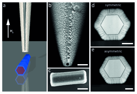
Figure 1: Experimental setup. (a) Schematic drawing showing the scanning SOT, a FNT lying on the substrate, and the direction of $\mathbf{H_{0}}$. The CoFeB shell is depicted in blue and the GaAs core in red. Pb on the SOT is shown in white. SEMs of the (b) the SOT tip and (c) a 0.7-$\mu$m-long FNT. (d) and (e) show cross-sectional HAADF STEMs of two FNTs from a similar growth batch as those measured. The scalebars represent 200 nm in (b) and (c) and 50 nm in (d) and (e).

We use a scanning SQUID-on-tip (SOT) sensor to map the stray field produced by FNTs as a function of position and applied field. We fabricate the SOT by evaporating Pb on the apex of a pulled quartz capillary according to a self-aligned method pioneered by Finkler et al. and perfected by Vasyukov et al. Finkler et al. (2010); Vasyukov et al. (2013). The SOT used here has an effective diameter of 150 nm, as extracted from measurements of the critical current $I_{\text{SOT}}$ as a function of a uniform magnetic field $\mathbf{H_{0}}=H_{0}\hat{z}$ applied perpendicular to the SQUID loop. At the operating temperature of 4.2 K, pronounced oscillations of critical current are visible as a function of $H_{0}$ up to 1 T. The SOT is mounted in a custom-built scanning probe microscope operating under vacuum in a ⁴He cryostat. Maps of the magnetic stray field produced by individual FNTs are made by scanning the FNTs lying on the substrate in the $xy$-plane 300 nm below the SOT sensor, as shown schematically in Fig. 1 (a). The current response of the sensor is proportional to the magnetic flux threaded through the SQUID loop. For each value of the externally applied field $H_{0}$, a factor is extracted from the current-field interference pattern to convert the measured current $I_{SOT}$ to the flux. The measured flux then represents the integral of the $z$-component of the total magnetic field over the area of the SQUID loop. By subtracting the contribution of $H_{0}$, we isolate the $z$-component of stray field, $H_{dz}$ integrated over the area of the SOT at each spatial position.

FNT samples consist of a non-magnetic GaAs core surrounded by a 30-nm-thick magnetic shell of CoFeB with hexagonal cross-section. CoFeB is magnetron-sputtered onto template GaAs nanowires (NWs) to produce an amorphous and homogeneous shell Gross et al. (2016), which is designed to avoid magneto-crystalline anisotropy Hindmarch et al. (2008); Rüffer et al. (2014); Schwarze and Grundler (2013). Nevertheless, recent magneto-transport experiments show that a small growth-induced magnetic anisotropy may be present Baumgaertl et al. (2016). Scanning electron micrographs (SEMs) of the studied FNTs, as in Fig. 1 (c), reveal continuous and defect-free surfaces, whose roughness is less than 5 nm. Figs. 1 (d) and (e) show cross-sectional high-angle annular dark-field (HAADF) scanning transmission electron micrographs (STEM) of two FNTs from the same growth batch as those measured, highlighting the possibility for asymmetry due to the deposition process. Dynamic cantilever magnetometry measurements of representative FNTs show $\mu_{0}M_{S}=1.3\pm 0.1$ T Gross et al. (2016), where $\mu_{0}$ is the permeability of free space and $M_{S}$ is the saturation magnetization. Their diameter $d$, which we define as the diameter of the circle circumscribing the hexagonal cross-section, is between 200 and 300 nm. Lengths from 0.7 to 4 $\mu$m are obtained by cutting individual FNTs into segments using a focused ion beam (FIB). After cutting, the FNTs are aligned horizontally on a patterned Si substrate. All stray-field progressions are measured as functions of $H_{0}$, which is applied perpendicular to the substrate and therefore perpendicular to the long axes of each FNT. Gross et al. found that similar CoFeB FNTs are fully saturated by a perpendicular field for $|\mu_{0}H_{0}|>1.2$ T at $T=4.2$ K Gross et al. (2016). Since the superconducting SQUID amplifier used in our measurement only allows measurements for $|\mu_{0}H_{0}|\leq 0.6$ T, all the progressions measured here represent minor hysteresis loops.

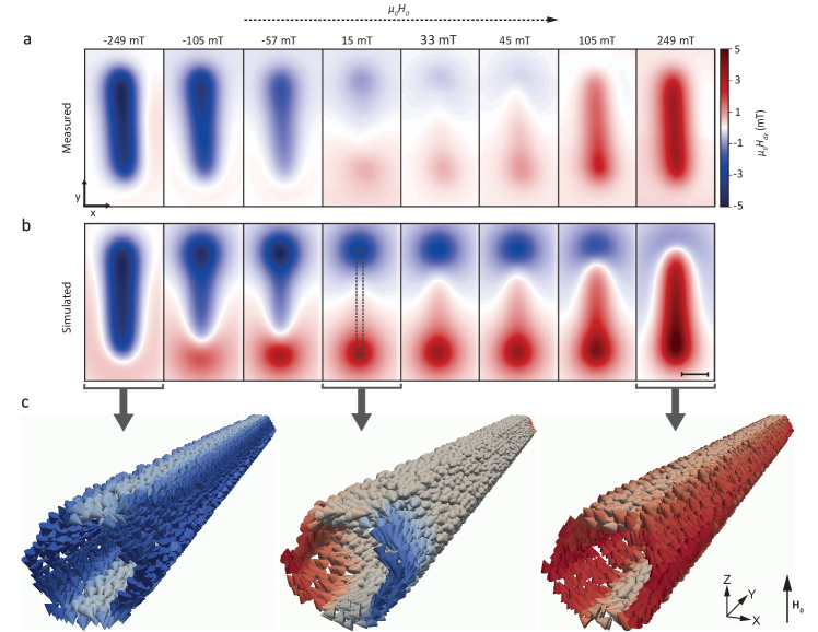
Figure 2: Magnetic reversal of a 4-$\mu$m-long FNT ($l=4.08$ $\mu$m, $d=260$ nm) in a field $H_{0}$ applied perpendicular to its long axis. Images of the stray field component along $\hat{z}$, $H_{dz}$, in the $xy$-plane 300 nm above the FNT for the labeled values of $\mu_{0}H_{0}$ (a) as measured by the scanning SOT and (b) as generated by numerical simulations of the equilibrium magnetization configuration. The dashed line deliniates the position of the FNT. The scalebar corresponds to 1 $\mu$m. (c) Simulated configurations corresponding to three values of $H_{0}$. The middle configuration, nearest to zero field, shows a mixed state with vortex end domains of opposing circulation sense. Arrows indicate the direction of the magnetization, while red (blue) contrast corresponds to the magnetization component along $\hat{z}$ ($-\hat{z}$).

Fig. 2 (a) shows the stray field maps of a 4-$\mu$m-long FNT for a series of fields as $\mu_{0}H_{0}$ is increased from -0.6 to 0.6 T. The maps reveal a reversal process roughly consistent with a rotation of the net FNT magnetization. At $\mu_{0}H_{0}=-249$ mT and at more negative fields , $H_{dz}$ is nearly uniform above the FNT, indicating that its magnetization is initially aligned along the applied field and thus parallel to $-\hat{z}$. As the field is increased toward positive values, maps of $H_{dz}$ show an average magnetization $\langle\mathbf{M}\rangle$, which rotates toward the long axis of the FNT. Near $H_{0}=0$, the two opposing stray field lobes at the ends of the FNT are consistent with an $\langle\mathbf{M}\rangle$ aligned along the long axis. With increasing positive $H_{0}$, the reversal proceeds until the magnetization aligns along $\hat{z}$.

The simulated stray-field maps, shown in Fig. 2 (b), are generated by a numerical micromagnetic model of the equilibrium magnetization configurations. We use the software package Mumax3 Vansteenkiste et al. (2014), which employs the Landau-Lifshitz micromagnetic formalism with finite-difference discretization. The length $l=4.08$ $\mu$m and diameter $d=260$ nm of the FNT are determined by SEMs of the sample, while the thickness $t=30$ nm is taken from cross-sectional TEMs of samples from the same batch. As shown in Fig. 2, the simulated stray-field distributions closely match the measurements. The magnetization configurations extracted from the simulations are non-uniform, as shown in Fig. 2 (c). In the central part of the FNT, the magnetization of the different facets in the hexagonal FNT rotates separately as a function of $H_{0}$, due to their shape anisotropy and their different orientations. As $H_{0}$ approaches zero, vortices nucleate at the FNT ends, resulting in a low-field mixed state, i.e. a configuration in which magnetization in the central part of the FNT aligns along its long axis and curls into azimuthally-aligned vortex domains at the ends. Experimental evidence for such end vortices has recently been observed by XMCD-PEEM Wyss et al. (2017) and DCM Mehlin (2017) measurements of similar FNTs at room-temperature. We also measured and simulated a 2-$\mu$m-long FNT of similar cross-sectional dimensions. It shows an analogous progression of stray field maps as a function of $H_{0}$ (see supplementary material). Simulations suggest a similar progression of magnetization configurations, with a mixed state in remnance.

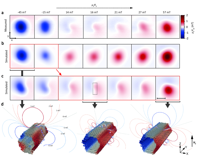
Figure 3: Magnetic reversal of a 0.7-$\mu$m-long FNT ($l=0.69$ $\mu$m, $d=250$ nm) in a field applied perpendicular to its long axis. Images of the stray field component along $\hat{z}$, $H_{dz}$, in the $xy$-plane 300 nm above the FNT for the labeled values of $H_{0}$ (a) as measured by the scanning SOT. (b) and (c) show numerical simulations of $H_{dz}$ produced by two progressions of equilibrium magnetization configurations with different initial conditions. The dashed line deliniates the position of the FNT and the scalebar corresponds to 0.5 $\mu$m. (c) Magnetization configurations and contours of constant $H_{dz}$ corresponding to three values of $H_{0}$. The configuration on the left is characterized by two vortices in the top and bottom facets, respectively. The middle and left configurations are distorted global vortex states. Arrows indicate the direction of the magnetization, while red (blue) contrast corresponds to the magnetization component along $\hat{z}$ ($-\hat{z}$).

FNTs shorter than 2 $\mu$m exhibit qualitatively different stray-field progressions. Measurements of a 0.7-$\mu$m-long FNT are shown in Fig. 3 (a). A stray-field pattern with a single lobe persists from large negative field to $\mu_{0}H_{0}=-15\leavevmode\nobreak\ \text{mT}$ without an indication of $\langle\mathbf{M}\rangle$ rotating towards the long axis. Near zero field, a stray-field map characterized by an ’S’-like zero-field line appears (white contrast in Fig. 3 (a)). At more positive fields, a single lobe again dominates. A similar progression of stray field images is also observed upon the reversal of a 1-$\mu$m-long FNT (not shown).

In order to infer the magnetic configuration of the FNT, we simulate its equilibrium configuration as a function of $H_{0}$ using the sample’s measured parameters: $l=0.69$ $\mu$m, $d=250$ nm and $t=30$ nm. For a perfectly hexagonal FNT with flat ends, the simulated reversal proceeds through different, slightly distorted global vortex states, which depend on the initial conditions of the magnetization. Such simulations do not reproduce the ’S’-like zero-field line observed in the measured stray-field maps. However, when we consider defects and structural asymmetries likely to be present in the measured FNT, the simulated and measured images come into agreement.

In these refined simulations, we first consider the magnetic ’dead-layer’ induced by the FIB cutting of the FNT ends as previously reported Katine et al. (2003); Khizroev and Litvinov (2004); Knutson (2008). We therefore reduce the length of the simulated FNT by 100 nm on either side. Second, we take into account that the FIB-cut ends of the FNT are not perfectly perpendicular to its long axis. SEMs of the investigated FNT show that the FIB cutting process results in ends slanted by $10^{\circ}$ with respect to $\hat{z}$. Finally, we consider that the 30-nm-thick hexagonal magnetic shell may be asymmetric, i.e. slightly thicker on one side of the FNT due to an inhomogeneous deposition, e.g. Fig. 1 (e).

With these modifications, the simulated reversal proceeds through at least four different possible stray-field progressions depending on the initial conditions. Only two of these, shown in Figs. 3 (b) and (c), produce stray-field maps which resemble the measurement. The measured stray-field images are consistent with the series shown in Fig. 3 (b) for negative fields ($\mu_{0}H_{0}=-45,-15\leavevmode\nobreak\ \text{mT}$). As the applied field crosses zero ($-15\leavevmode\nobreak\ \text{mT}\leq\mu_{0}H_{0}\leq 14\leavevmode\nobreak\ \text{mT}$), the FNT appears to change stray-field progressions. The images taken at positive fields ($14\leavevmode\nobreak\ \text{mT}\leq\mu_{0}H_{0}$), show patterns consistent with the series shown in Fig. 3 (c). The magnetic configurations corresponding to these simulated stray-field maps suggest that the FNT occupies a slightly distorted global vortex state. Before entering this state, e.g. at $\mu_{0}H_{0}=-45\leavevmode\nobreak\ \text{mT}$, the simulations show a more complex configuration with magnetic vortices in the top and bottom facets, rather than at the FNT ends. On the other hand, at similar reverse fields, e.g. $\mu_{0}H_{0}=57\leavevmode\nobreak\ \text{mT}$, the FNT is shown to occupy a distortion of the global vortex state with an tilt of the magnetization toward the FNT long axis in some of the hexagonal facets.

For some minor loop measurements of short FNTs ($l\leq 1$ $\mu$m), we obtain stray-field patterns, which the micromagnetic simulations do not reproduce. Two such cases are shown in Fig. 4, where (a) represents the stray-field pattern measured above a 0.7-$\mu$m-long FNT at $\mu_{0}H_{0}=20\leavevmode\nobreak\ \text{mT}$ and (d) the pattern measured above a 1-$\mu$m FNT at $\mu_{0}H_{0}=21\leavevmode\nobreak\ \text{mT}$. Both of these stray-field maps are qualitatively different from the results of Fig. 3. Since the simulations do not provide equilibrium magnetization configurations that generate these measured stray-field patterns, we test a few idealized configurations in search of possible matches. In particular, the measured pattern shown in Fig. 4 (a) is similar to the pattern produced by an opposing vortex state. This configuration, shown in Fig. 4 (c), consists of two vortices of opposing circulation sense, separated by a domain wall. It was observed with XMCD-PEEM to occur in similar-sized FNTs Wyss et al. (2017) in remnance at room-temperature. The pattern measured in Fig. 4 (e) appears to match the stray-field produced by a multi-domain state consisting of two head-to-head axial domains separated by a vortex domain wall and capped by two vortex ends, shown in Fig. 4 (f). Although these configurations are not calculated to be equilibrium states for these FNTs in a perpendicular field, they have been suggested as possible intermediate states during reversal of axial magnetization in a longitudinal field Landeros et al. (2007). The presence of these anomalous configurations in our experiments may be due to incomplete magnetization saturation or imperfections not taken into account by our numerical model.

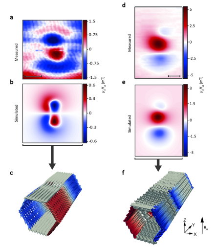
Figure 4: Anomalous stray-field patterns found at low applied field. (a) Stray-field pattern of the 0.7-$\mu$m-long FNT ($l=0.69$ $\mu$m, $d=250$ nm) at $\mu_{0}H_{0}=20\leavevmode\nobreak\ \text{mT}$. (b) Similar map produced by an opposing vortex state, shown schematically in (c) and observed near zero field by Wyss et al. Wyss et al. (2017). (d) Stray-field pattern of the 1-$\mu$m-long FNT ($l=1.05$ $\mu$m, $d=250$ nm) at $\mu_{0}H_{0}=21\leavevmode\nobreak\ \text{mT}$. (e) Similar field map produced by a (f) multi-domain mixed state with vortex end domains and opposing axial domains separated by a vortex wall. The scalebar corresponds to 0.5 $\mu$m. In (c) and (f), arrows indicate the direction of the magnetization, while red (blue) contrast corresponds to the magnetization component along $\hat{z}$

Wyss et al. showed that the types of remnant states that emerge in CoFeB FNTs depend on their length Wyss et al. (2017). For FNTs of these cross-sectional dimensions longer than 2 $\mu$m, the equilibrium remnant state at room temperature is the mixed state, while shorter FNTs favor global or opposing vortex states. Here, we confirm these observations at cyrogenic temperatures by mapping the magnetic stray-field produced by the FNTs rather than their magnetization. In this way, we directly image the defining property of flux-closure configurations, i.e. the extent to which their stray field vanishes. In fact, we find that the imperfect geometry of the FNTs causes even the global vortex state to produce stray fields on the order of 100 $\mu$T at a distance of 300 nm. Finer control of the sample geometry is required in order to reduce this stray field and for such devices be considered as elements in ultra-high density magnetic storage. Using the scanning SQUID’s ability to make images as a function of applied magnetic field, we also reveal the progression of stray-field patterns produced by the FNTs as they reverse their magnetization. Future scanning SOT experiments in parallel applied fields could further test the applicability of established theory to real FNTs Usov et al. (2007); Landeros et al. (2007, 2009); Landeros and Núñez (2010). While the incomplete flux closure and the presence of magnetization configurations not predicted by simulation indicate that FNT samples still cannot be considered ideal, scanning SOT images show the promise of using geometry to program both the overall equilibrium magnetization configurations and the reversal process in nanomagnets.

Methods. SOT Fabrication. SOTs were fabricated according to the technique described by Vasyukov et al. Vasyukov et al. (2013) using a three-step evaporation of Pb on the apex of a quartz capillary, pulled to achieve the required SOT diameter. The evaporation was performed in a custom-made evaporator with a base pressure of $2\times 10^{-8}$ mbar and a rotateable sample holder cooled by liquid He. In accordance with Halbertal et al. Halbertal et al. (2016), an additional Au shunt was deposited close to the tip apex prior to the Pb evaporation for protection of the SOTs against electrostatic discharge. SOTs were characterized in a test setup prior to their use in the scanning probe microscope.

SOT Positioning and Scanning. Positioning and scanning of the sample below the SOT is carried out using piezo-electric positioners and scanners (Attocube AG). We use the sensitivity of the SOT to both temperature and magnetic field Halbertal et al. (2016) in combination with electric current, which is passed through a serpentine conductor on the substrate, to position specific FNTs under the SOT (see supplementary material).

FNT Sample Preparation. The template NWs, onto which the CoFeB shell is sputtered, are grown by molecular beam epitaxy on a Si (111) substrate using Ga droplets as catalysts Rüffer et al. (2014). During CoFeB sputter deposition, the wafers of upright and well-separated GaAs NWs are mounted with a 35^∘ angle between the long axis of the NWs and the deposition direction. The wafers are then continuously rotated in order to achieve a conformal coating. In order to obtain NTs with different lengths and well-defined ends, we cut individual NTs into segments using a Ga FIB in a scanning electron microscope. After cutting, we use an optical microscope equipped with precision micromanipulators to pick up the FNT segments and align them horizontally onto a Si substrate. FNT cross-sections for the HAADF STEMs were also prepared using a FIB.

Mumax3 Simulations. To simulate the CoFeB FNTs, we set $\mu_{0}M_{S}$ to its measured value of $1.3\text{\,}\mathrm{T}$ and the exchange stiffness to $A_{ex}=$28\text{\,}\mathrm{pJ}$/$\mathrm{m}$$. The external field is intentionally tilted by $2^{\circ}$ with respect to $\hat{z}$ in both the $xz$- and the $yz$-plane, in order to exclude numerical artifacts due to symmetry. This angle is within our experimental alignment error. The asymmetry in the magnetic cross-section of an FNT, seen in Fig. 1 (e), is generated by removing a hexagonal core from a larger hexagonal wire, whose axis is slightly shifted. In this case, the wire’s diameter is 30 nm larger than the core’s diameter and we shift the core’s axis below that of the wire by 5 nm. In order to rule out spurious effects due to the discretization of the numerical cells, the cell size must be smaller than the ferromagnetic exchange length of 6.5 nm. This criterion is fulfilled by using a 5-nm cell size to simulate the 0.7-$\mu$m-long FNT. For the 4-$\mu$m-long FNT, computational limitations force us to set the cell size to 8 nm, such that the full scanning field can be calculated in a reasonable amount of time. Given that the cell size exceeds the exchange length, the results are vulnerable to numerical artifacts. To confirm the reliability of these simulations, we perform a reference simulation with a 4-nm cell size. Although the magnetic states are essentially unchanged by the difference in cell size, the value of the stray field is altered by up to 10%.