Magnetic dipole moment of $Z_{b}(10610)$ in light-cone QCD

Abstract

The magnetic dipole moment of the exotic $Z_{b}(10610)$ state is calculated within the light cone QCD sum rule method using the diquark-antidiquark and molecule interpolating currents. The magnetic dipole moment is obtained as $\mu_{Z_{b}}=1.73\pm 0.63~{}\mu_{N}$ in diquark-antidiquark picture and $\mu_{Z_{b}}=1.59\pm 0.58~{}\mu_{N}$ in the molecular case. The obtained results in both pictures together with the results of other theoretical studies on the spectroscopic parameters of the $Z_{b}(10610)$ state may be useful in determination of the nature and quark organization of this state.

I Introduction

According to QCD and the conventional quark model, not only the standard hadrons, but also exotic states such as meson-baryon molecules, tetraquarks, pentaquarks, glueball and hybrids can exist. The first theoretical prediction on the existence of the multiquark structures was made by Jaffe in 1976 Jaffe:1976ih . Although it was predicted in the 1970’s, there was not significant experimental evidence of their existence until 2003. The first observation on the exotic states was discovery of $X(3872)$ made by Belle Collaboration Choi:2003ue in the decay $B^{+}\rightarrow K^{+}X(3872)J/\psi\pi^{+}\pi^{-}$. Subsequently, it was confirmed by BABAR Aubert:2004ns , CDF II Acosta:2003zx , D0 Abazov:2004kp , LHCb Aaij:2011sn and CMS Chatrchyan:2013cld Collaborations. The discovery of the X(3872) state turned out to be the forerunner of a new direction in hadron physics. So far, more than twenty exotic states have been observed experimentally [for details, see Nielsen:2009uh ; Swanson:2006st ; Voloshin:2007dx ; Klempt:2007cp ; Godfrey:2008nc ; Faccini:2012pj ; Esposito:2014rxa ; Ali:2017jda ]. The failure of these states to fit the standard particles’ structures and violation of some conservation laws such as isospin symmetry, make these states suitable tools for studying the nonperturbative nature of QCD.

In 2011, Belle Collaboration discovered two charged bottomonium-like states $Z_{b}(10610)$ and $Z_{b}(10650)$ (hereafter we will denote these states as $Z_{b}$ and $Z_{b}^{\prime}$, respectively) in the processes $\Upsilon(5S)\rightarrow\pi\pi\Upsilon(nS)$, and$\Upsilon(5S)\rightarrow\pi\pi h_{b}(kP)$ Belle:2011aa . Here, n = 1, 2, 3 and k = 1, 2. The masses and widths of the two states have been measured as

$$M_{Z_{b}}=10607.2\pm 2~{}MeV,~{}~{}~{}~{}\Gamma_{Z_{b}}=18.4\pm 2.4~{}MeV,$$

$$M_{Z_{b}^{\prime}}=10652.2\pm 1.5~{}MeV,~{}~{}~{}~{}\Gamma_{Z_{b}^{\prime}}=11.5\pm 2.2~{}MeV.$$

The analysis of the angular distribution shows that the quantum numbers of both states are $I^{G}(J^{P})=1^{+}(1^{+})$. Both $Z_{b}$ and $Z_{b}^{\prime}$ belong to the family of charged hidden-bottom states. Since they are the first observed charged bottomoniumlike states and also very close to the thresholds of $B\bar{B}^{*̄}(10604.6MeV)$ and $B^{*}\bar{B}^{*}(10650.2MeV)$, $Z_{b}$ and $Z_{b}^{\prime}$ states have attracted attention of many theoretical groups. The spectroscopic parameters and decays of $Z_{b}$ and $Z_{b}^{\prime}$ states have been studied with different models and approaches. Most of these investigations are based on diquark-antidiquark Cui:2011fj ; Ali:2011ug ; Agaev:2017lmc ; Wang:2013zra and molecular interpretations Cui:2011fj ; Bondar:2011ev ; Voloshin:2011qa ; Zhang:2011jja ; Yang:2011rp ; Sun:2011uh ; Chen:2011zv ; Chen:2011pv ; Cleven:2011gp ; Cleven:2013sq ; Mehen:2013mva ; Wang:2013daa ; Wang:2014gwa ; Dong:2012hc ; Chen:2015ata ; Kang:2016ezb ; Goerke:2017svb ; Dias:2014pva ; Li:2012wf ; Li:2012as ; Xiao:2017uve ; Huo:2015uka , using the analogy to the charm sector. Although the spectroscopic features of these states have been studied sufficiently, the inner structure of these states have not exactly enlightened. Different kinds of analyses, such as interaction with the photon can shed light on the internal structure of these multiquark states.

A comprehensive analysis of the electromagnetic properties of hadrons ensures crucial information on the nonperturbative nature of QCD and their geometric shapes. The electromagnetic multipole moments contain the spatial distributions of the charge and magnetization in the particle and therefore, these observables are directly related to the spatial distributions of quarks and gluons in hadrons. In this study, the magnetic dipole moment of the exotic state $Z_{b}$ is extracted by using the diquark-antidiquark and molecule interpolating currents in the framework of the light cone QCD sum rule (LCSR). This method has already been successfully applied to study the dynamical and statical properties of hadrons for decades such as, form factors, coupling constants and multipole moments. In the LCSR, the properties of the particles are characterized in terms of the light-cone distribution amplitudes (DAs) and the vacuum condensates [for details, see for instance Chernyak:1990ag ; Braun:1988qv ; Balitsky:1989ry ].

The rest of the paper is organized as follows: In Sec. II, the light-cone QCD sum rule for the electromagnetic form factors of $Z_{b}$ is applied and its magnetic dipole moment is derived. Section III, encompasses our numerical analysis and discussion. The explicit expressions of the photon DAs are moved to the Appendix A.

II Formalism

To obtain the magnetic dipole moment of the $Z_{b}$ state by using the LCSR approach, we begin with the subsequent correlation function,

$$\Pi_{\mu\nu\alpha}(p,q)=i^{2}\int d^{4}x\,\int d^{4}y\,e^{ip\cdot x+iq\cdot y}\,\langle 0|\mathcal{T}\{J_{\mu}^{Z_{b}}(x)J_{\alpha}(y)J_{\nu}^{Z_{b}\dagger}(0)\}|0\rangle.$$ (1)

Here, $J_{\mu(\nu)}$ is the interpolating current of the $Z_{b}$ state and the electromagnetic current $J_{\alpha}$ is given as,

$$J_{\alpha}=\sum_{q=u,d,b}e_{q}\bar{q}\gamma_{\alpha}q,$$ (2)

where $e_{q}$ is the electric charge of the corresponding quark.

From technical point of view, it is more convenient to rewrite the correlation function by using the external background electromagnetic (BGEM) field,

$$\Pi_{\mu\nu}(p,q)=i\int d^{4}x\,e^{ip\cdot x}\langle 0|\mathcal{T}\{J_{\mu}^{Z_{b}}(x)J_{\nu}^{Z_{b}\dagger}(0)\}|0\rangle_{F},$$ (3)

where F is the external BGEM field and $F_{\alpha\beta}=i(\varepsilon_{\alpha}q_{\beta}-\varepsilon_{\beta}q_{\alpha})$ with $q_{\alpha}$ and $\varepsilon_{\beta}$ being the four-momentum and polarization of the BGEM field. Since the external BGEM field can be made arbitrarily small, the correlation function in Eq. (3) can be acquired by expanding in powers of the BGEM field,

$$\Pi_{\mu\nu}(p,q)=\Pi_{\mu\nu}^{(0)}(p,q)+\Pi_{\mu\nu}^{(1)}(p,q)+....,$$ (4)

and keeping only terms $\Pi_{\mu\nu}^{(1)}(p,q)$, which corresponds to the single photon emission Ioffe:1983ju ; Ball:2002ps (the technical details about the external BGEM field method can be found in Novikov:1983gd ). The main advantage of using the BGEM field approach relies on the fact that it separates the soft and hard photon emissions in an explicitly gauge invariant way Ball:2002ps . The $\Pi_{\mu\nu}^{(0)}(p,q)$ is the correlation function in the absence of the BGEM field, and gives rise to the mass sum rules of the hadrons, which is not relevant for our case.

After these general remarks, we can now proceed deriving the LCSR for the magnetic dipole moment of the $Z_{b}$ state. The correlation function given in Eq. (3) can be obtained in terms of hadronic parameters, known as hadronic representation. Additionally it can be calculated in terms of the quark and gluon parameters in the deep Euclidean region, known as QCD representation.

We can insert a complete set of intermediate hadronic states with the same quantum numbers as the interpolating current of the $Z_{b}$ into the correlation function to obtain the hadronic representation. Then, by isolating the ground state contributions, we obtain the following expression:

$$\Pi_{\mu\nu}^{Had}(p,q)={\frac{\langle 0\mid J_{\mu}^{Z_{b}}\mid Z_{b}(p)\rangle}{p^{2}-m_{Z_{b}}^{2}}}\langle Z_{b}(p)\mid Z_{b}(p+q)\rangle_{F}\frac{\langle Z_{b}(p+q)\mid{J^{\dagger}}_{\nu}^{Z_{b}}\mid 0\rangle}{(p+q)^{2}-m_{Z_{b}}^{2}}+\cdots,$$ (5)

where dots denote the contributions coming from the higher states and continuum.

The matrix element appearing in Eq. (5) can be written in terms of three invariant form factors as follows Brodsky:1992px :

$$\langle Z_{b}(p,\varepsilon^{\theta})\mid Z_{b}(p+q,\varepsilon^{\delta})\rangle_{F} =-\varepsilon^{\tau}(\varepsilon^{\theta})^{\alpha}(\varepsilon^{\delta})^{\beta}\Bigg{[}G_{1}(Q^{2})~{}(2p+q)_{\tau}~{}g_{\alpha\beta}+G_{2}(Q^{2})~{}(g_{\tau\beta}~{}q_{\alpha}-g_{\tau\alpha}~{}q_{\beta})$$

$$-\frac{1}{2m_{Z_{b}}^{2}}G_{3}(Q^{2})~{}(2p+q)_{\tau}~{}q_{\alpha}q_{\beta}\Bigg{]}\,,$$ (6)

where $\varepsilon^{\tau}$ is the polarization vector of the BGEM field; and $\varepsilon^{\theta}$ and $\varepsilon^{\delta}$ are the polarization vectors of the initial and final $Z_{b}$ states.

The remaining matrix element, that of the interpolating current between the vacuum and particle state, $\langle 0\mid J_{\mu}^{Z_{b}}\mid Z_{b}\rangle$, is parametrized as

$$\langle 0\mid J_{\mu}^{Z_{b}}\mid Z_{b}\rangle=\lambda_{Z_{b}}\varepsilon_{\mu}^{\theta}\,,$$ (7)

where $\lambda_{Z_{b}}$ is residue of the $Z_{b}$ state.

The form factors $G_{1}(Q^{2})$, $G_{2}(Q^{2})$ and $G_{3}(Q^{2})$ can be defined in terms of the charge $F_{C}(Q^{2})$, magnetic $F_{M}(Q^{2})$ and quadrupole $F_{\cal D}(Q^{2})$ form factors as follows

$$F_{C}(Q^{2})=G_{1}(Q^{2})+\frac{2}{3}(Q^{2}/4m_{Z_{b}}^{2})F_{\cal D}(Q^{2})\,,$$

$$F_{M}(Q^{2})=G_{2}(Q^{2})\,,$$

$$F_{\cal D}(Q^{2})=G_{1}(Q^{2})-G_{2}(Q^{2})+(1+Q^{2}/4m_{Z_{b}}^{2})G_{3}(Q^{2})\,,$$ (8)

At $Q^{2}=0$, the form factors $F_{C}(Q^{2}=0)$, $F_{M}(Q^{2}=0)$, and $F_{\cal D}(Q^{2}=0)$ are related to the electric charge, magnetic moment $\mu$ and the quadrupole moment ${\cal D}$ as

$$eF_{C}(0)=e\,,$$

$$eF_{M}(0)=2m_{Z_{b}}\mu\,,$$

$$eF_{\cal D}(0)=m_{Z_{b}}^{2}{\cal D}\,.$$ (9)

Inserting the matrix elements in Eqs. (II) and (7) into the correlation function in Eq. (5) and imposing the condition $q\!\cdot\!\varepsilon=0$, we obtain the correlation function in terms of the hadronic parameters as

$$\Pi_{\mu\nu}^{Had}(p,q) =\lambda_{Z_{b}}^{2}\frac{\varepsilon^{\tau}}{[m_{Z_{b}}^{2}-(p+q)^{2}][m_{Z_{b}}^{2}-p^{2}]}\Bigg{[}2p_{\tau}F_{C}(0)\Bigg{(}g_{\mu\nu}-\frac{p_{\mu}q_{\nu}-p_{\nu}q_{\mu}}{m_{Z_{b}}^{2}}\Bigg{)}$$

$$+F_{M}(0)\Bigg{(}q_{\mu}g_{\nu\tau}-q_{\nu}g_{\mu\tau}+\frac{1}{m_{Z_{b}}^{2}}p_{\tau}(p_{\mu}q_{\nu}-p_{\nu}q_{\mu})\Bigg{)}-\Bigg{(}F_{C}(0)+F_{\cal D}(0)\Bigg{)}{\frac{p_{\tau}}{m_{Z_{b}}^{2}}}q_{\mu}q_{\nu}\Bigg{]}\,.$$ (10)

To obtain the expression of the correlation function in terms of the quark and gluon parameters, the explicit form for the interpolating current of the $Z_{b}$ state needs to be chosen. In this study, we consider the $Zb$ state with the quantum numbers $J^{PC}=1^{+-}$. Then in the diquark-antidiquark model the interpolating current $J_{\mu}^{Z_{b}}$ is defined by the following expression in terms of quark fields:

$$J_{\mu}^{Z_{b}(Di)}(x) = \frac{i\epsilon\tilde{\epsilon}}{\sqrt{2}}\left\{\left[u_{a}^{T}(x)C\gamma_{5}b_{b}(x)\right]\left[\overline{d}_{d}(x)\gamma_{\mu}C\overline{b}_{e}^{T}(x)\right]-\left[u_{a}^{T}(x)C\gamma_{\mu}b_{b}(x)\right]\left[\overline{d}_{d}(x)\gamma_{5}C\overline{b}_{e}^{T}(x)\right]\right\},$$ (11)

where $C$ is the charge conjugation matrix, $\epsilon=\epsilon_{abc}$, $\tilde{\epsilon}=\epsilon_{dec}$; and $a,b,...$ are color indices.

One can also construct the interpolating current by considering the $Z_{b}$ as a molecular form of $B\bar{B}^{*}$ and $B^{*}\bar{B}$ state,

$$J_{\mu}^{Zb(Mol)}(x) = \frac{1}{\sqrt{2}}\Big{\{}[\bar{d}_{a}(x)i\gamma_{5}b_{a}(x)][\bar{b}_{b}(x)\gamma_{\mu}u_{b}(x)]+[\bar{d}_{a}(x)\gamma_{\mu}b_{a}(x)][\bar{b}_{b}(x)i\gamma_{5}u_{b}(x)]\Big{\}}.$$ (13)

After contracting pairs of the light and heavy quark operators, the correlation function becomes:

$$\Pi_{\mu\nu}^{\mathrm{QCD}}(p,q) = -i\frac{\epsilon\tilde{\epsilon}\epsilon^{\prime}\tilde{\epsilon}^{\prime}}{2}\int d^{4}xe^{ipx}\langle 0|\Bigg{\{}\mathrm{Tr}\Big{[}\gamma_{5}\widetilde{S}_{u}^{aa^{\prime}}(x)\gamma_{5}S_{c}^{bb^{\prime}}(x)\Big{]}\mathrm{Tr}\Big{[}\gamma_{\mu}\widetilde{S}_{c}^{e^{\prime}e}(-x)\gamma_{\nu}S_{d}^{d^{\prime}d}(-x)\Big{]}$$ (14)

$$-\mathrm{Tr}\Big{[}\gamma_{\mu}\widetilde{S}_{c}^{e^{\prime}e}(-x)\gamma_{5}S_{d}^{d^{\prime}d}(-x)\Big{]}\mathrm{Tr}\Big{[}\gamma_{\nu}\widetilde{S}_{u}^{aa^{\prime}}(x)\gamma_{5}S_{c}^{bb^{\prime}}(x)]$$

$$-\mathrm{Tr}\Big{[}\gamma_{5}\widetilde{S}_{u}^{a^{\prime}a}(x)\gamma_{\mu}S_{c}^{b^{\prime}b}(x)\Big{]}\mathrm{Tr}\Big{[}\gamma_{5}\widetilde{S}_{c}^{e^{\prime}e}(-x)\gamma_{\nu}S_{d}^{d^{\prime}d}(-x)\Big{]}$$

$$+\mathrm{Tr}\Big{[}\gamma_{\nu}\widetilde{S}_{u}^{aa^{\prime}}(x)\gamma_{\mu}S_{c}^{bb^{\prime}}(x)\Big{]}\mathrm{Tr}\Big{[}\gamma_{5}\widetilde{S}_{c}^{e^{\prime}e}(-x)\gamma_{5}S_{d}^{d^{\prime}d}(-x)\Big{]}\Bigg{\}}|0\rangle_{F},$$

in the diquark-antidiquark picture, and

$$\Pi_{\mu\nu}^{\mathrm{QCD}}(p,q) = -\frac{i}{2}\int d^{4}xe^{ipx}\langle 0|\Bigg{\{}\mathrm{Tr}\Big{[}\gamma_{5}{S}_{b}^{aa^{\prime}}(x)\gamma_{5}S_{d}^{a^{\prime}a}(-x)\Big{]}\mathrm{Tr}\Big{[}\gamma_{\mu}{S}_{u}^{bb^{\prime}}(x)\gamma_{\nu}S_{b}^{b^{\prime}b}(-x)\Big{]}$$ (15)

$$+\mathrm{Tr}\Big{[}\gamma_{5}{S}_{b}^{aa^{\prime}}(x)\gamma_{\nu}S_{d}^{a^{\prime}a}(-x)\Big{]}\mathrm{Tr}\Big{[}\gamma_{\mu}{S}_{u}^{bb^{\prime}}(x)\gamma_{5}S_{b}^{b^{\prime}b}(-x)]$$

$$+\mathrm{Tr}\Big{[}\gamma_{\mu}{S}_{b}^{aa^{\prime}}(x)\gamma_{5}S_{d}^{a^{\prime}a}(-x)\Big{]}\mathrm{Tr}\Big{[}\gamma_{5}{S}_{u}^{bb^{\prime}}(x)\gamma_{\nu}S_{b}^{b^{\prime}b}(-x)\Big{]}$$

$$+\mathrm{Tr}\Big{[}\gamma_{\mu}{S}_{b}^{aa^{\prime}}(x)\gamma_{\nu}S_{d}^{a^{\prime}a}(-x)\Big{]}\mathrm{Tr}\Big{[}\gamma_{5}{S}_{u}^{bb^{\prime}}(x)\gamma_{5}S_{b}^{b^{\prime}b}(-x)\Big{]}\Bigg{\}}|0\rangle_{F},$$

in the molecular picture, where

$$\widetilde{S}_{b(q)}(x)=CS_{b(q)}^{\mathrm{T}}(x)C,$$

with $S_{q}(x)$ and $S_{b}(x)$ being the light and heavy quark propagators, respectively. To calculate the correlation functions in QCD representations, the light and heavy quark propagators are required. Their explicit expressions in the $x$-space are given as

$$S_{q}(x)=i\frac{{x\!\!\!/}}{2\pi^{2}x^{4}}-\frac{\langle\bar{q}q\rangle}{12}\Big{(}1+\frac{m_{0}^{2}x^{2}}{16}\Big{)}-\frac{ig_{s}}{32\pi^{2}x^{2}}G^{\mu\nu}(x)\Big{[}\hbox to0.0pt{/\hss}{x}\sigma_{\mu\nu}+\sigma_{\mu\nu}\hbox to0.0pt{/\hss}{x}\Big{]},$$ (16)

and

$$S_{b}(x)=\frac{m_{b}^{2}}{4\pi^{2}}\Bigg{[}\frac{K_{1}\Big{(}m_{b}\sqrt{-x^{2}}\Big{)}}{\sqrt{-x^{2}}}+i\frac{{x\!\!\!/}~{}K_{2}\Big{(}m_{b}\sqrt{-x^{2}}\Big{)}}{(\sqrt{-x^{2}})^{2}}\Bigg{]}-\frac{g_{s}m_{b}}{16\pi^{2}}\int_{0}^{1}dv\,G^{\mu\nu}(vx)\Bigg{[}(\sigma_{\mu\nu}{x\!\!\!/}+{x\!\!\!/}\sigma_{\mu\nu})\frac{K_{1}\Big{(}m_{b}\sqrt{-x^{2}}\Big{)}}{\sqrt{-x^{2}}}$$

$$+2\sigma_{\mu\nu}K_{0}\Big{(}m_{b}\sqrt{-x^{2}}\Big{)}\Bigg{]},$$ (17)

where $K_{i}$ are the second kind Bessel functions, $v$ is line variable and $G^{\mu\nu}$ is the gluon field strength tensor.

The correlation function includes different types of contributions. In first case, one of the free quark propagators in Eqs. (14-15) is replaced by

$$S^{free}\rightarrow\int d^{4}y\,S^{free}(x-y)\,\hbox to0.0pt{/\hss}{\!A}(y)\,S^{free}(y)\,,$$ (18)

where $S^{free}$ is the first term of the light or heavy quark propagators and the remaining three propagators are replaced with the full quark propagators. The LCSR calculations are most conveniently done in the fixed-point gauge. For electromagnetic field, it is defined by $x_{\mu}A^{\mu}=0$. In this gauge, the electromagnetic potential is given by

$$A_{\alpha}=-\frac{1}{2}F_{\alpha\beta}y^{\beta}=-\frac{1}{2}(\varepsilon_{\alpha}q_{\beta}-\varepsilon_{\beta}q_{\alpha})\,y^{\beta}.$$ (19)

The Eq. (19) is plugged into Eq. (18), as a result of which we obtain

$$S^{free}\rightarrow-\frac{1}{2}(\varepsilon_{\alpha}q_{\beta}-\varepsilon_{\beta}q_{\alpha})\int\,d^{4}y\,y^{\beta}\,S^{free}(x-y)\,\gamma_{\alpha}\,S^{free}(y)\,,$$ (20)

After some calculations for $S_{q}^{free}$ and $S_{b}^{free}$ we get

$$S_{q}^{free}=\frac{e_{q}}{32\pi^{2}x^{2}}\Bigg{(}\varepsilon_{\alpha}q_{\beta}-\varepsilon_{\beta}q_{\alpha}\Bigg{)}\Bigg{(}x\!\!\!/\sigma_{\alpha\beta}+\sigma_{\alpha\beta}x\!\!\!/\Bigg{)},$$

$$S_{b}^{free}=-i\frac{e_{b}m_{b}}{32\pi^{2}}\Bigg{(}\varepsilon_{\alpha}q_{\beta}-\varepsilon_{\beta}q_{\alpha}\Bigg{)}\Bigg{[}2\sigma_{\alpha\beta}K_{0}\Big{(}m_{b}\sqrt{-x^{2}}\Big{)}+\frac{K_{1}\Big{(}m_{b}\sqrt{-x^{2}}\Big{)}}{\sqrt{-x^{2}}}\Bigg{(}x\!\!\!/\sigma_{\alpha\beta}+\sigma_{\alpha\beta}x\!\!\!/\Bigg{)}\Bigg{]}.$$ (21)

In second case one of the light quark propagators in Eqs. (14-15) are replaced by

$$S_{\alpha\beta}^{ab}\rightarrow-\frac{1}{4}(\bar{q}^{a}\Gamma_{i}q^{b})(\Gamma_{i})_{\alpha\beta},$$ (22)

and the remaining propagators are full quark propagators including the perturbative as well as the nonperturbative contributions. Here as an example, we give a short detail of the calculations of the QCD representations. In second case for simplicity, we only consider the first term in Eq. (14),

$$\Pi_{\mu\nu}^{\mathrm{QCD}}(p,q)=-i\frac{\epsilon\tilde{\epsilon}\epsilon^{\prime}\tilde{\epsilon}^{\prime}}{2}\int d^{4}xe^{ipx}\langle 0|\mathrm{Tr}\Big{[}\gamma_{5}\widetilde{S}_{u}^{aa^{\prime}}(x)\gamma_{5}S_{b}^{bb^{\prime}}(x)\Big{]}\mathrm{Tr}\Big{[}\gamma_{\mu}\widetilde{S}_{b}^{e^{\prime}e}(-x)\gamma_{\nu}S_{d}^{d^{\prime}d}(-x)\Big{]}|0\rangle_{F}+...$$ (23)

By replacing one of light propagators with the expressions in Eq. (22) and making use of

$$\bar{q}^{a}(x)\Gamma_{i}q^{a^{\prime}}(0)\rightarrow\frac{1}{3}\delta^{aa^{\prime}}\bar{q}(x)\Gamma_{i}q(0),$$ (24)

the Eq. (23) takes the form

$$\Pi_{\mu\nu}^{\mathrm{QCD}}(p,q)=-i\frac{\epsilon\tilde{\epsilon}\epsilon^{\prime}\tilde{\epsilon}^{\prime}}{2}\int d^{4}xe^{ipx}\Bigg{\{}\mathrm{Tr}\Big{[}\gamma_{5}\Gamma_{i}\gamma_{5}S_{b}^{bb^{\prime}}(x)\Big{]}\mathrm{Tr}\Big{[}\gamma_{\mu}\widetilde{S}_{b}^{e^{\prime}e}(-x)\gamma_{\nu}S_{d}^{d^{\prime}d}(-x)\Big{]}\frac{1}{12}\delta^{aa^{\prime}}$$

$$+\mathrm{Tr}\Big{[}\gamma_{5}\widetilde{S}_{u}^{aa^{\prime}}(x)\gamma_{5}S_{b}^{bb^{\prime}}(x)\Big{]}\mathrm{Tr}\Big{[}\gamma_{\mu}\widetilde{S}_{b}^{e^{\prime}e}(-x)\gamma_{\nu}\Gamma_{i}\Big{]}\frac{1}{12}\delta^{dd^{\prime}}\Bigg{\}}\langle\gamma(q)|\bar{q}(x)\Gamma_{i}q(0)|0\rangle+...,$$ (25)

where $\Gamma_{i}=I,\gamma_{5},\gamma_{\mu},i\gamma_{5}\gamma_{\mu},\sigma_{\mu\nu}/2$. Similarly, when a light propagator interacts with the photon, a gluon may be released from one of the remaining three propagators. The expression obtained in this case is as follows:

$$\Pi_{\mu\nu}^{\mathrm{QCD}}(p,q)=-i\frac{\epsilon\tilde{\epsilon}\epsilon^{\prime}\tilde{\epsilon}^{\prime}}{2}\int d^{4}xe^{ipx}\Bigg{\{}\mathrm{Tr}\Big{[}\gamma_{5}\Gamma_{i}\gamma_{5}S_{b}^{bb^{\prime}}(x)\Big{]}\mathrm{Tr}\Big{[}\gamma_{\mu}\widetilde{S}_{b}^{e^{\prime}e}(-x)\gamma_{\nu}S_{d}^{d^{\prime}d}(-x)\Big{]}\Big{[}\Big{(}\delta^{ab}\delta^{a^{\prime}b^{\prime}}-\frac{1}{3}\delta^{aa^{\prime}}\delta^{bb^{\prime}}\Big{)}$$

$$+\Big{(}\delta^{ae}\delta^{a^{\prime}e^{\prime}}-\frac{1}{3}\delta^{aa^{\prime}}\delta^{ee^{\prime}}\Big{)}+\Big{(}\delta^{ad}\delta^{a^{\prime}d^{\prime}}-\frac{1}{3}\delta^{aa^{\prime}}\delta^{dd^{\prime}}\Big{)}\Big{]}$$

$$+\mathrm{Tr}\Big{[}\gamma_{5}\widetilde{S}_{u}^{aa^{\prime}}(x)\gamma_{5}S_{b}^{bb^{\prime}}(x)\Big{]}\mathrm{Tr}\Big{[}\gamma_{\mu}\widetilde{S}_{b}^{e^{\prime}e}(-x)\gamma_{\nu}\Gamma_{i}\Big{]}\Big{[}\Big{(}\delta^{db}\delta^{d^{\prime}b^{\prime}}-\frac{1}{3}\delta^{dd^{\prime}}\delta^{bb^{\prime}}\Big{)}+\Big{(}\delta^{de}\delta^{d^{\prime}e^{\prime}}-\frac{1}{3}\delta^{dd^{\prime}}\delta^{ee^{\prime}}\Big{)}$$

$$+\Big{(}\delta^{ad}\delta^{a^{\prime}d^{\prime}}-\frac{1}{3}\delta^{aa^{\prime}}\delta^{dd^{\prime}}\Big{)}\Big{]}\Bigg{\}}\frac{1}{32}\langle\gamma(q)|\bar{q}(x)\Gamma_{i}G_{\mu\nu}(vx)q(0)|0\rangle+...,$$ (26)

where we inserted

$$\bar{q}^{a}(x)\Gamma_{i}G_{\mu\nu}^{bb^{\prime}}(vx)q^{a^{\prime}}(0)\rightarrow\frac{1}{8}\Big{(}\delta^{ab}\delta^{a^{\prime}b^{\prime}}-\frac{1}{3}\delta^{aa^{\prime}}\delta^{bb^{\prime}}\Big{)}\bar{q}(x)\Gamma_{i}G_{\mu\nu}(vx)q(0).$$ (27)

As is seen, there appear matrix elements such as $\langle\gamma(q)\left|\bar{q}(x)\Gamma_{i}q(0)\right|0\rangle$ and $\langle\gamma(q)\left|\bar{q}(x)\Gamma_{i}G_{\mu\nu}(vx)q(0)\right|0\rangle$, representing the nonperturbative contributions. These matrix elements can be expressed in terms of photon DAs and wave functions with definite twists, whose expressions are given in Appendix A. The QCD representation of the correlation function is obtained by using Eqs. (14-27). Then, the Fourier transformation is applied to transfer expressions in x-space to the momentum space.

The sum rule for the magnetic dipole moment are obtained by matching the expressions of the correlation function in terms of QCD parameters and its expression in terms of the hadronic parameters, using their spectral representation. To eliminate the contributions of the excited and continuum states in the spectral representation of the correlation function, a double Borel transformation with respect to the variables $p^{2}$ and $(p+q)^{2}$ is applied. After the transformation, these contributions are exponentially suppressed. Eventually, we choose the structure $(\varepsilon.p)(p_{\mu}q_{\nu}-q_{\mu}p_{\nu})$ for the magnetic dipole moment and obtain

$$\mu^{Di}=\frac{e^{m_{Z_{b}}^{2}/M^{2}}}{\lambda_{Z_{b}}^{2}m_{Z_{b}}^{2}}\Bigg{[}\Pi_{1}+\Pi_{2}\Bigg{]},$$ (28)

$$\mu^{Mol}=\frac{e^{m_{Z_{b}}^{2}/M^{2}}}{\lambda_{Z_{b}}^{2}m_{Z_{b}}^{2}}\Bigg{[}\Pi_{3}+\Pi_{4}\Bigg{]}.$$ (29)

The explicit forms of the functions that appear in the above sum rules are given as follows:

$$\Pi_{1} = \frac{3m_{b}^{4}}{256\pi^{6}}(e_{u}-e_{d})\Bigg{\{}32N[3,3,0]-2M^{2}N[3,3,1]-16m_{b}N[3,4,1]+m_{b}M^{2}N[3,4,2]\Bigg{\}}$$

$$-\frac{m_{b}^{2}\langle g_{s}^{2}G^{2}\rangle}{9216\pi^{6}}(e_{u}-e_{d})\Bigg{(}-M^{2}N[1,1,0]+2m_{b}N[1,2,0]\Bigg{)}$$

$$-\frac{m_{b}^{2}\langle g_{s}^{2}G^{2}\rangle}{147456\pi^{6}}\Bigg{(}2m_{b}M^{2}N[1,2,1]+\pi^{2}\langle\bar{q}q\rangle\Big{(}16N[1,2,1]+5N[1,2,2]\Big{)}\Bigg{)}$$

$$+\frac{m_{b}^{4}\langle g_{s}^{2}G^{2}\rangle}{294912\pi^{6}}(e_{u}-e_{d})\Bigg{(}16N[1,3,1]-M^{2}N[1,3,2]\Bigg{)}$$

$$-\frac{m_{b}^{2}\langle g_{s}^{2}G^{2}\rangle}{294912\pi^{6}}(e_{u}-e_{d})\Bigg{(}128N[2,2,0]-8(2m_{b}^{2}+M^{2})N[2,2,1]+m_{b}^{2}M^{2}N[2,2,2]\Bigg{)}$$

$$-\frac{m_{b}^{3}}{98304\pi^{6}}(e_{u}-e_{d})\Bigg{(}16\Big{(}\langle g_{s}^{2}G^{2}\rangle-192\pi^{2}m_{b}\langle\bar{q}q\rangle\Big{)}N[2,3,1]+M^{2}\Big{(}13\langle g_{s}^{2}G^{2}\rangle-960\pi^{2}m_{b}\langle\bar{q}q\rangle\Big{)}N[2,3,2]$$

$$-\frac{m_{b}^{3}m_{0}^{2}\langle\bar{q}q\rangle}{384M^{8}\pi^{4}}(e_{u}+e_{d})\Bigg{(}64m_{b}^{6}FlP[-3,4,0]-48m_{b}^{4}FlP[-2,4,0]+12m_{b}^{2}FlP[-1,4,0]-FlP[0,4,0]\Bigg{)}$$

$$-\frac{m_{b}m_{0}^{2}\langle g_{s}^{2}G^{2}\rangle\langle\bar{q}q\rangle}{36864M^{8}\pi^{4}}(e_{u}-e_{d})\Bigg{(}16m_{b}^{4}FlP[-1,2,0]-8m_{b}^{2}FlP[0,2,0]+FlP[1,2,0]\Bigg{)},$$

$$\Pi_{2}=-\frac{m_{b}\langle g_{s}^{2}G^{2}\rangle\langle\bar{q}q\rangle^{2}}{2592M^{10}\pi^{2}}(e_{u}-e_{d})(m_{0}^{2}-M^{2})I_{3}[h_{\gamma}]\Bigg{(}4m_{b}^{2}FlNP[0,1,0]-FlNP[-1,1,0]\Bigg{)}$$

$$+\frac{m_{b}m_{0}^{2}\langle g_{s}^{2}G^{2}\rangle\langle\bar{q}q\rangle^{2}}{10368M^{10}\pi^{2}}(e_{u}-e_{d})I_{3}[h_{\gamma}]\Bigg{(}4m_{b}^{2}FlNP[2,1,1]-FlNP[3,1,1]\Bigg{)}$$

$$-\frac{f_{3\gamma}m_{0}^{2}\langle g_{s}^{2}G^{2}\rangle\langle\bar{q}q\rangle}{110592M^{10}\pi^{2}}\Big{[}-(4e_{u}-3e_{d})\psi^{a}(u_{0})+2e_{d}I_{3}[\psi^{\nu}]\Big{]}\Bigg{(}16m_{b}^{4}FlNP[1,2,1]-8m_{b}^{2}FlNP[2,2,1]$$

$$+FlNP[3,2,1]\Bigg{)}$$

$$-\frac{m_{b}m_{0}^{2}\langle g_{s}^{2}G^{2}\rangle\langle\bar{q}q\rangle}{995328M^{12}\pi^{2}}(8e_{u}-5e_{d})(A(u_{0})+8I_{3}[h_{\gamma}])\Bigg{(}16m_{b}^{4}FlNP[2,3,2]-8m_{b}^{2}FlNP[3,3,2]+FlNP[4,3,2]\Bigg{)}$$

$$+\frac{m_{b}\langle\bar{q}q\rangle^{2}}{497664M^{12}\pi^{2}}(8e_{u}-5e_{d})\Bigg{[}-\langle g_{s}^{2}G^{2}\rangle\Big{(}-(5m_{0}^{2}-2M^{2})A(u_{0})-2m_{0}^{2}\chi M^{2}\varphi_{\gamma}(u_{0})\Big{)}-8\Big{\{}-5m_{0}^{2}\langle g_{s}^{2}G^{2}\rangle$$

$$+2\Big{(}M^{2}\langle g_{s}^{2}G^{2}\rangle+432m_{b}^{2}m_{0}^{2}M^{2}\Big{)}I_{3}[h_{\gamma}]\Big{\}}\Bigg{]}\Bigg{(}16m_{b}^{4}FlNP[0,3,1]-8m_{b}^{2}FlNP[1,3,1]+FlNP[2,3,1]\Bigg{)}$$

$$+\frac{m_{b}}{165888M^{10}\pi^{4}}\Bigg{[}(e_{u}-e_{d})f_{3\gamma}\Big{(}7M^{2}\langle g_{s}^{2}G^{2}\rangle-576\pi^{2}m_{b}\langle\bar{q}q\rangle(m_{0}^{2}-M^{2})\Big{)}\psi^{a}(u_{0})+72\pi^{2}\langle\bar{q}q\rangle^{2}(m_{0}^{2}-M^{2})$$

$$\Big{(}-2e_{u}I_{1}[\tilde{S}]+e_{d}\Big{(}3I_{2}[\mathcal{T}_{1}]-3I_{2}[\mathcal{T}_{2}]-5I_{2}[\tilde{S}]\Big{)}\Big{)}\Bigg{]}\Bigg{(}-64m_{b}^{6}FlNP[3,4,0]+48m_{b}^{4}FlNP[2,4,0]$$

$$-12m_{b}^{2}FlNP[1,4,0]+FlNP[0,4,0]\Bigg{)}$$

$$-\frac{m_{b}m_{0}^{2}\langle\bar{q}q\rangle}{9216M^{10}\pi^{4}}\Bigg{[}-8(e_{u}-e_{d})m_{b}f_{3\gamma}\psi^{a}(u_{0})-\langle\bar{q}q\rangle\Big{(}-2e_{u}I_{1}[\tilde{S}]+e_{d}\Big{(}3I_{2}[\mathcal{T}_{1}]-3I_{2}[\mathcal{T}_{2}]-5I_{2}[\tilde{S}]\Big{)}\Big{)}\Bigg{]}$$

$$\Bigg{(}64m_{b}^{6}FlNP[-1,4,1]-48m_{b}^{4}FlNP[0,4,1]+12m_{b}^{2}FlNP[1,4,1]-FlNP[2,4,1]\Bigg{)}$$

$$+\frac{\langle\bar{q}q\rangle}{1990656M^{12}\pi^{4}}\Bigg{[}\langle g_{s}^{2}G^{2}\rangle\Bigg{\{}2e_{u}\Bigg{(}-3M^{4}\Big{(}16m_{b}^{4}FlNP[1,3,0]-8m_{b}^{2}FlNP[0,3,0]+FlNP[-1,3,0]\Big{)}$$

$$-32\pi^{2}m_{b}\langle\bar{q}q\rangle(5m_{0}^{2}-4M^{2})\Big{(}16m_{b}^{4}FlNP[2,3,0]-8m_{b}^{2}FlNP[1,3,0]+FlNP[0,3,0]\Big{)}\Bigg{)}$$

$$+e_{d}\Bigg{(}40\pi^{2}m_{b}\langle\bar{q}q\rangle(5m_{0}^{2}-4M^{2})\Big{(}16m_{b}^{4}FlNP[2,3,0]-8m_{b}^{2}FlNP[1,3,0]+FlNP[0,3,0]\Big{)}$$

$$+3M^{4}\Big{(}-48m_{b}^{6}FlNP[2,3,0]+56m_{b}^{4}FlNP[1,3,0]-19m_{b}^{2}FlNP[0,3,0]+2FlNP[-1,3,0]\Big{)}\Bigg{)}\Bigg{\}}A(u_{0})$$

$$+8m_{b}\Bigg{\{}-4(8e_{u}-5e_{d})\pi^{2}M^{2}\chi\langle g_{s}^{2}G^{2}\rangle\langle\bar{q}q\rangle(m_{0}^{2}-M^{2})\varphi_{\gamma}(u_{0})-3(40e_{u}-43e_{d})m_{b}M^{4}\langle g_{s}^{2}G^{2}\rangle$$

$$+8(8e_{u}-5e_{d})\pi^{2}\langle g_{s}^{2}G^{2}\rangle\langle\bar{q}q\rangle(5m_{0}^{2}-M^{2})-432(e_{u}-e_{d})\pi^{2}m_{b}^{2}M^{2}\langle\bar{q}q\rangle(m_{0}^{2}-4M^{2})\Bigg{\}}I_{3}[h_{\gamma}]\Bigg{]}$$

$$\Big{(}16m_{b}^{4}FlNP[2,3,0]-8m_{b}^{2}FlNP[1,3,0]+FlNP[0,3,0]\Big{)},$$ (31)

$$\Pi_{3} = \frac{9m_{b}^{4}}{1024\pi^{6}}(e_{u}-e_{d})\Bigg{\{}32N[3,3,0]-2M^{2}N[3,3,1]-16m_{b}N[3,4,1]+m_{b}M^{2}N[3,4,2]\Bigg{\}}$$ (32)

$$-\frac{m_{b}^{3}}{32768\pi^{6}}(e_{u}-e_{d})(\langle g_{s}^{2}G^{2}\rangle+48\pi^{2}m_{b}\langle\bar{q}q\rangle)\Bigg{(}16N[2,3,1]+5M^{2}N[2,3,2]\Bigg{)}$$

$$-\frac{m_{b}^{3}m_{0}^{2}\langle\bar{q}q\rangle}{512M^{8}\pi^{2}}(e_{u}-e_{d})\Bigg{(}64m_{b}^{6}4FlP[-3,4,0]-48m_{b}^{4}FlP[-2,4,0]+12m_{b}^{2}FlP[-1,4,0]+FlP[0,4,0]\Bigg{)},$$

and

$$\Pi_{4} = \frac{m_{b}^{2}\langle g_{s}^{2}G^{2}\rangle\langle\bar{q}q\rangle}{294912\pi^{4}}\Bigg{[}e_{u}\Big{(}-3I_{1}[\mathcal{S}]-2I_{1}[\tilde{S}]\Big{)}+e_{d}\Big{(}3I_{2}[\mathcal{S}]+2I_{2}[\tilde{S}]\Big{)}\Bigg{]}\Bigg{(}M^{2}N[1,2,2]-8N[1,2,1]\Bigg{)}$$ (33)

$$+\frac{3m_{b}^{2}\langle\bar{q}q\rangle}{64\pi^{4}}(e_{u}-e_{d})I_{3}[h_{\gamma}]\Bigg{(}M^{2}N[2,3,2]-8N[2,3,1]\Bigg{)}+\frac{3m_{b}^{4}f_{3\gamma}}{128\pi^{4}}(e_{u}+e_{d})\psi^{a}(u_{0})\Bigg{(}M^{2}N[3,3,2]-8N[3,3,1]\Bigg{)}$$

$$-\frac{m_{b}^{3}m_{0}^{2}\langle\bar{q}q\rangle^{2}}{96M^{10}\pi^{2}}(e_{u}-e_{d})I_{3}[h_{\gamma}]\Bigg{(}64m_{b}^{6}FlNP[0,3,1]-48m_{b}^{4}FlNP[1,3,1]+FlNP[2,3,1]\Bigg{)}$$

$$-\frac{m_{b}^{3}m_{0}^{2}f_{3\gamma}\langle\bar{q}q\rangle^{2}}{1536M^{10}\pi^{2}}(e_{u}-e_{d})\psi^{a}(u_{0})\Bigg{(}64m_{b}^{6}FlNP[-1,4,1]-48FlNP[0,4,1]+12m_{b}^{2}FlNP[1,4,1]$$

$$-FlNP[2,4,1]\Bigg{)}$$

$$+\frac{m_{b}f_{3\gamma}}{18432M^{10}\pi^{4}}(e_{u}+e_{d})\Bigg{[}\Big{(}-M^{2}\langle g_{s}^{2}G^{2}\rangle-48\pi^{2}m_{b}\langle\bar{q}q\rangle(m_{0}^{2}-M^{2})\Big{)}\psi^{a}(u_{0})\Bigg{]}\Bigg{(}-64m_{b}^{6}FlNP[3,4,0]$$

$$+48m_{b}^{4}FlNP[2,4,0]-12m_{b}^{2}FlNP[1,4,0]+FlNP[0,4,0]\Bigg{)}$$

$$-\frac{m_{b}\langle\bar{q}q\rangle}{1152M^{10}\pi^{4}}(e_{u}-e_{d})\Bigg{[}\Big{(}-M^{2}\langle g_{s}^{2}G^{2}\rangle-48\pi^{2}m_{b}\langle\bar{q}q\rangle(m_{0}^{2}-M^{2})\Big{)}I_{3}[h_{\gamma}]\Bigg{]}\Bigg{(}-16m_{b}^{4}FlNP[2,3,0]$$

$$-8m_{b}^{2}FlNP[1,3,0]+FlNP[0,3,0]\Bigg{)}.$$

where, $m_{b}$ is the mass of the b quark, $e_{q}$ is the corresponding electric charge, $\chi$ is the magnetic susceptibility of the quark condensate, $m_{0}^{2}=\langle\bar{q}g\sigma_{\alpha\beta}G^{\alpha\beta}q\rangle/\langle\bar{q}q\rangle$, $\langle\bar{q}q\rangle$ and $\langle g_{s}^{2}G^{2}\rangle$ are quark and gluon condensates, respectively.

The functions $N[n,m,k]$, $FlP[n,m,k]$, $FlNP[n,m,k]$,  $I_{1}[\mathcal{A}]$,  $I_{2}[\mathcal{A}]$ and $I_{3}[\mathcal{A}]$ are defined as:

$$N[n,m,k] =\int_{0}^{\infty}dt\int_{0}^{\infty}dt^{\prime}~{}\frac{e^{-m_{b}/2(t+t^{\prime})}}{t^{n}~{}(\frac{m_{b}}{t}+\frac{m_{b}}{t^{\prime}})^{k}~{}t^{\prime m}},$$

$$FlP[n,m,k] =\int_{4m_{b}^{2}}^{s_{0}}ds\int_{4m_{b}^{2}}^{s}dl~{}\frac{e^{-l^{2}/\phi}~{}l^{n}~{}(l-s)^{m}}{(4m_{b}^{2}-l)^{2}~{}\phi^{k}},$$

$$FlNP[n,m,k] =\int_{4m_{b}^{2}}^{s_{0}}ds\int_{4m_{b}^{2}}^{s}dl~{}\frac{e^{-l^{2}/\beta}~{}l^{n}~{}(l-s)^{m}}{(l-2m_{b}^{2})~{}\beta^{k}},$$

$$I_{1}[\mathcal{A}] =\int D_{\alpha_{i}}\int_{0}^{1}dv~{}\mathcal{A}(\alpha_{\bar{q}},\alpha_{q},\alpha_{g})\delta(\alpha_{q}+\bar{v}\alpha_{g}-u_{0}),$$

$$I_{2}[\mathcal{A}] =\int D_{\alpha_{i}}\int_{0}^{1}dv~{}\mathcal{A}(\alpha_{\bar{q}},\alpha_{q},\alpha_{g})\delta(\alpha_{\bar{q}}+v\alpha_{g}-u_{0}),$$

$$I_{3}[\mathcal{A}] =\int_{0}^{1}du~{}A(u),$$

where

$$\beta=4\,l\,M^{2}-16\,m_{b}^{2}M^{2},$$

$$\phi=8\,l\,M^{2}-32\,m_{b}^{2}M^{2}.$$

The functions $\Pi_{1}$ and $\Pi_{3}$ indicate the case that one of the quark propagators enters the perturbative interaction with the photon and the remaining three propagators are taken as full propagators. The functions $\Pi_{2}$ and $\Pi_{4}$ show the contributions that one of the light quark propagators enters the nonperturbative interaction with the photon and the remaining three propagators are taken as full propagators. The reader can find some details about the calculations such as Fourier and Borel transformations as well as continuum subtraction in Appendix C of Ref. Ozdem:2017jqh .

As we already mentioned, the calculations have been done in the fixed-point gauge, $x_{\mu}A^{\mu}=0$, for simplicity. In order to show whether our results are gauge invariant or not we examine the Lorentz gauge, $\partial_{\mu}A^{\mu}=0$. In this gauge, the electromagnetic vector potential is written as

$$A_{\mu}(x)=\varepsilon_{\mu}e^{-iq.x},$$ (35)

with $\varepsilon_{\mu}q^{\mu}=0$. In this gauge, the corresponding gauge invariant electromagnetic field strength tensor is written as

$$F_{\mu\nu}=i(\varepsilon_{\mu}q_{\nu}-q_{\mu}\varepsilon_{\nu})e^{-iq.x}.$$ (36)

We repeat all the calculations in this gauge and find the same results for the magnetic dipole moment of the state under consideration. Therefore the results obtained in the present study are gauge invariant.

III Numerical analysis and Conclusion

In this section, we numerically analyze the results of calculations for magnetic dipole moment of the $Z_{b}$ state. We use $m_{Z_{b}}=10607.2\pm 2MeV$, $\overline{m}_{b}(m_{b})=(4.18_{-0.03}^{+0.04})~{}GeV$ Olive:2016xmw , $f_{3\gamma}=-0.0039~{}GeV^{2}$ Ball:2002ps , $\langle\bar{q}q\rangle(1\,GeV)=(-0.24\pm 0.01)^{3}\,GeV^{3}$ Ioffe:2005ym , $m_{0}^{2}=0.8\pm 0.1~{}GeV^{2}$, $\langle g_{s}^{2}G^{2}\rangle=0.88~{}GeV^{4}$ Nielsen:2009uh and $\chi(1\,GeV)=-2.85\pm 0.5~{}GeV^{-2}$ Rohrwild:2007yt . To evaluate a numerical prediction for the magnetic moment, we need also specify the values of the residue of the $Z_{b}$ state. The residue is obtained from the mass sum rule as $\lambda_{Z_{b}}=m_{Z_{b}}f_{Z_{b}}$ with $f_{Z_{b}}=(2.79^{+0.55}_{-0.65})\times 10^{-2}~{}GeV^{4}$ Agaev:2017lmc for diquark-antidiquark picture and $\lambda_{Z_{b}}=0.27\pm 0.07~{}GeV^{5}$ Zhang:2011jja for molecular picture. The parameters used in the photon DAs are given in Appendix A, as well.

The estimations for the magnetic dipole moment of the $Z_{b}$ state depend on two auxiliary parameters; the continuum threshold $s_{0}$ and Borel mass parameter $M^{2}$. The continuum threshold is not completely an arbitrary parameter, and there are some physical restrictions for it. The $s_{0}$ signals the scale at which, the excited states and continuum start to contribute to the correlation function. The working interval for this parameter is chosen such that the maximum pole contribution is acquired and the results relatively weakly depend on its choices. Our numerical calculations lead to the interval $[119-128]~{}GeV^{2}$ for this parameter. The Borel parameter can vary in the interval that the results weakly depend on it according to the standard prescriptions. The upper bound of it is found demanding the maximum pole contributions and its lower bound is found the convergence of the operator product expansion and exceeding of the perturbative part over nonperturbative contributions. Under these constraints, the working region of the Borel parameter is determined as $15~{}GeV^{2}\leq M^{2}\leq 17~{}GeV^{2}$.

In Fig. 1, we plot the dependency of the magnetic dipole moment of the $Z_{b}$ state on $M^{2}$ at different fixed values of the continuum threshold. From the figure we observe that the results considerably depend on the variations of the Borel parameter. The magnetic dipole moment is stable under variation of $s_{0}$ in its working region. In Fig. 2, we show the contributions of $\Pi_{1}$, $\Pi_{2}$, $\Pi_{3}$ and $\Pi_{4}$ functions to the results obtained at average value of $s_{0}$ with respect to the Borel mass parameter. It is clear that $\Pi_{1}$ is dominant in the results obtained when using diquark-antidiquark current but $\Pi_{3}$ is dominant while using the molecular current. The contribution of the $\Pi_{2}$ and $\Pi_{4}$ functions seems to be almost zero. When the results are analyzed in detail, almost (95-97)% of the total contribution comes from the perturbative part and the remaining (3-5)% belongs to the nonperturbative contributions.

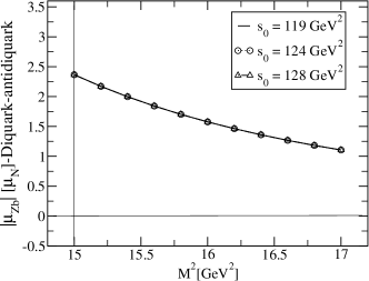
(a)

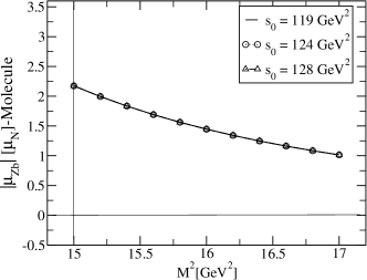
(b)

Figure 1: The dependence of the magnetic moment for $Z_{b}$ state; on the Borel parameter squared $M^{2}$ at different fixed values of the continuum threshold.

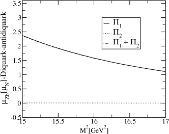
(a)

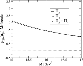
(b)

Figure 2: Comparison of the contributions to the magnetic moment with respect to $M^{2}$ at average value of $s_{0}$.

Our predictions on the numerical value of the magnetic dipole moment in both pictures are presented in Table I. The errors in the results come from the variations in the calculations of the working regions of $M^{2}$ and from the uncertainties in the values of the input parameters as well as the photon DAs. We shall remark that the main source of uncertainties is the variations with respect to variations of $M^{2}$.

Picture	$|\mu_{Z_{b}}|$
Diquark-antidiquark	1.73$\pm$ 0.63
Molecule	1.59$\pm$ 0.58

Table 1: Results of the magnetic moment (in units of $\mu_{N}$) for $Z_{b}$ state.

In conclusion, we have computed the magnetic dipole moment of the $Z_{b}(10610)$ by modeling it as the diquark-antidiquark and molecule states. In our calculations we have employed the light-cone QCD sum rule in electromagnetic background field. Although the central values of the magnetic dipole moment obtained via two pictures differ slightly from each other but they are consistent within the errors. In Ref. Agaev:2017lmc , both the spectroscopic parameters and some of the strong decays of the $Z_{b}$ state have been studied using diquark-antidiquark interpolating current. Although the obtained mass in Agaev:2017lmc is in agreement with the experimental data, the result obtained for the width of $Z_{b}$ in the diquark-antidiquark picture in Agaev:2017lmc differ considerably from the experimental data. They suggested, as a result, that the $Z_{b}$ state may not have a pure diquark-antidiquark structure. When we combine the obtained results in the present study with those of the predictions on the mass obtained via both pictures in the literature and those result obtained for the width of $Z_{b}$ in Ref. Agaev:2017lmc we conclude that both pictures can be considered for the internal structure of $Z_{b}$. May be a mixed current will be a better choice for interpolating this particle. More theoretical and experimental studies are still needed to be performed in this respect.

Finally, the magnetic dipole moment encodes important information about the inner structure of particles and their geometric shape. The results obtained for the magnetic dipole moment of $Z_{b}$ state in both the diquark-antidiquark and molecule pictures, within a factor 2, are of the same order of magnitude as the proton’s magnetic moment and not such small that it appears hopeless to try to measure the value of the magnetic dipole moment of this state. By the recent progresses in the experimental side, we hope that we can measure the multipole moments of the newly founded exotic states, especially the $Z_{b}$ particle in future. Comparison of any experimental data on the magnetic dipole moment of $Z_{b}$ will be useful to gain exact knowledge on its quark organizations and will help us in the course of undestanding the structures of the newly observed exotic states and their quantum chromodynamics.

IV Acknowledgement

This work has been supported by the Scientific and Technological Research Council of Turkey (TÜBİTAK) under the Grant No. 115F183.

Appendix A: Photon DAs and Wave Functions

In this appendix, we present the definitions of the matrix elements of the forms $\langle\gamma(q)\left|\bar{q}(x)\Gamma_{i}q(0)\right|0\rangle$ and $\langle\gamma(q)\left|\bar{q}(x)\Gamma_{i}G_{\mu\nu}q(0)\right|0\rangle$ in terms of the photon DAs and wave functions Ball:2002ps ,

$$\langle\gamma(q)|\bar{q}(x)\gamma_{\mu}q(0)|0\rangle=e_{q}f_{3\gamma}\left(\varepsilon_{\mu}-q_{\mu}\frac{\varepsilon x}{qx}\right)\int_{0}^{1}due^{i\bar{u}qx}\psi^{v}(u)$$

$$\langle\gamma(q)|\bar{q}(x)\gamma_{\mu}\gamma_{5}q(0)|0\rangle=-\frac{1}{4}e_{q}f_{3\gamma}\epsilon_{\mu\nu\alpha\beta}\varepsilon^{\nu}q^{\alpha}x^{\beta}\int_{0}^{1}due^{i\bar{u}qx}\psi^{a}(u)$$

$$\langle\gamma(q)|\bar{q}(x)\sigma_{\mu\nu}q(0)|0\rangle=-ie_{q}\langle\bar{q}q\rangle(\varepsilon_{\mu}q_{\nu}-\varepsilon_{\nu}q_{\mu})\int_{0}^{1}due^{i\bar{u}qx}\left(\chi\varphi_{\gamma}(u)+\frac{x^{2}}{16}\mathbb{A}(u)\right)$$

$$-\frac{i}{2(qx)}e_{q}\bar{q}q\left[x_{\nu}\left(\varepsilon_{\mu}-q_{\mu}\frac{\varepsilon x}{qx}\right)-x_{\mu}\left(\varepsilon_{\nu}-q_{\nu}\frac{\varepsilon x}{qx}\right)\right]\int_{0}^{1}due^{i\bar{u}qx}h_{\gamma}(u)$$

$$\langle\gamma(q)|\bar{q}(x)g_{s}G_{\mu\nu}(vx)q(0)|0\rangle=-ie_{q}\langle\bar{q}q\rangle\left(\varepsilon_{\mu}q_{\nu}-\varepsilon_{\nu}q_{\mu}\right)\int{\cal D}\alpha_{i}e^{i(\alpha_{\bar{q}}+v\alpha_{g})qx}{\cal S}(\alpha_{i})$$

$$\langle\gamma(q)|\bar{q}(x)g_{s}\tilde{G}_{\mu\nu}(vx)i\gamma_{5}q(0)|0\rangle=-ie_{q}\langle\bar{q}q\rangle\left(\varepsilon_{\mu}q_{\nu}-\varepsilon_{\nu}q_{\mu}\right)\int{\cal D}\alpha_{i}e^{i(\alpha_{\bar{q}}+v\alpha_{g})qx}\tilde{\cal S}(\alpha_{i})$$

$$\langle\gamma(q)|\bar{q}(x)g_{s}\tilde{G}_{\mu\nu}(vx)\gamma_{\alpha}\gamma_{5}q(0)|0\rangle=e_{q}f_{3\gamma}q_{\alpha}(\varepsilon_{\mu}q_{\nu}-\varepsilon_{\nu}q_{\mu})\int{\cal D}\alpha_{i}e^{i(\alpha_{\bar{q}}+v\alpha_{g})qx}{\cal A}(\alpha_{i})$$

$$\langle\gamma(q)|\bar{q}(x)g_{s}G_{\mu\nu}(vx)i\gamma_{\alpha}q(0)|0\rangle=e_{q}f_{3\gamma}q_{\alpha}(\varepsilon_{\mu}q_{\nu}-\varepsilon_{\nu}q_{\mu})\int{\cal D}\alpha_{i}e^{i(\alpha_{\bar{q}}+v\alpha_{g})qx}{\cal V}(\alpha_{i})$$

$$\langle\gamma(q)|\bar{q}(x)\sigma_{\alpha\beta}g_{s}G_{\mu\nu}(vx)q(0)|0\rangle=e_{q}\langle\bar{q}q\rangle\left\{\left[\left(\varepsilon_{\mu}-q_{\mu}\frac{\varepsilon x}{qx}\right)\left(g_{\alpha\nu}-\frac{1}{qx}(q_{\alpha}x_{\nu}+q_{\nu}x_{\alpha})\right)\right.\right.q_{\beta}$$

$$-\left(\varepsilon_{\mu}-q_{\mu}\frac{\varepsilon x}{qx}\right)\left(g_{\beta\nu}-\frac{1}{qx}(q_{\beta}x_{\nu}+q_{\nu}x_{\beta})\right)q_{\alpha}-\left(\varepsilon_{\nu}-q_{\nu}\frac{\varepsilon x}{qx}\right)\left(g_{\alpha\mu}-\frac{1}{qx}(q_{\alpha}x_{\mu}+q_{\mu}x_{\alpha})\right)q_{\beta}$$

$$+\left.\left(\varepsilon_{\nu}-q_{\nu}\frac{\varepsilon x}{q.x}\right)\left(g_{\beta\mu}-\frac{1}{qx}(q_{\beta}x_{\mu}+q_{\mu}x_{\beta})\right)q_{\alpha}\right]\int{\cal D}\alpha_{i}e^{i(\alpha_{\bar{q}}+v\alpha_{g})qx}{\cal T}_{1}(\alpha_{i})$$

$$+\left[\left(\varepsilon_{\alpha}-q_{\alpha}\frac{\varepsilon x}{qx}\right)\left(g_{\mu\beta}-\frac{1}{qx}(q_{\mu}x_{\beta}+q_{\beta}x_{\mu})\right)\right.q_{\nu}$$

$$-\left(\varepsilon_{\alpha}-q_{\alpha}\frac{\varepsilon x}{qx}\right)\left(g_{\nu\beta}-\frac{1}{qx}(q_{\nu}x_{\beta}+q_{\beta}x_{\nu})\right)q_{\mu}$$

$$-\left(\varepsilon_{\beta}-q_{\beta}\frac{\varepsilon x}{qx}\right)\left(g_{\mu\alpha}-\frac{1}{qx}(q_{\mu}x_{\alpha}+q_{\alpha}x_{\mu})\right)q_{\nu}$$

$$+\left.\left(\varepsilon_{\beta}-q_{\beta}\frac{\varepsilon x}{qx}\right)\left(g_{\nu\alpha}-\frac{1}{qx}(q_{\nu}x_{\alpha}+q_{\alpha}x_{\nu})\right)q_{\mu}\right]\int{\cal D}\alpha_{i}e^{i(\alpha_{\bar{q}}+v\alpha_{g})qx}{\cal T}_{2}(\alpha_{i})$$

$$+\frac{1}{qx}(q_{\mu}x_{\nu}-q_{\nu}x_{\mu})(\varepsilon_{\alpha}q_{\beta}-\varepsilon_{\beta}q_{\alpha})\int{\cal D}\alpha_{i}e^{i(\alpha_{\bar{q}}+v\alpha_{g})qx}{\cal T}_{3}(\alpha_{i})$$

$$+\left.\frac{1}{qx}(q_{\alpha}x_{\beta}-q_{\beta}x_{\alpha})(\varepsilon_{\mu}q_{\nu}-\varepsilon_{\nu}q_{\mu})\int{\cal D}\alpha_{i}e^{i(\alpha_{\bar{q}}+v\alpha_{g})qx}{\cal T}_{4}(\alpha_{i})\right\}~{},$$

where $\varphi_{\gamma}(u)$ is the leading twist-2, $\psi^{v}(u)$, $\psi^{a}(u)$, ${\cal A}(\alpha_{i})$ and ${\cal V}(\alpha_{i})$, are the twist-3, and $h_{\gamma}(u)$, $\mathbb{A}(u)$, ${\cal S}(\alpha_{i})$, ${\cal{\tilde{S}}}(\alpha_{i})$, ${\cal T}_{1}(\alpha_{i})$, ${\cal T}_{2}(\alpha_{i})$, ${\cal T}_{3}(\alpha_{i})$ and ${\cal T}_{4}(\alpha_{i})$ are the twist-4 photon DAs. The measure ${\cal D}\alpha_{i}$ is defined as

$$\int{\cal D}\alpha_{i}=\int_{0}^{1}d\alpha_{\bar{q}}\int_{0}^{1}d\alpha_{q}\int_{0}^{1}d\alpha_{g}\delta(1-\alpha_{\bar{q}}-\alpha_{q}-\alpha_{g})~{}.$$

The expressions of the DAs entering into the above matrix elements are defined as:

$$\varphi_{\gamma}(u) = 6u\bar{u}\left(1+\varphi_{2}(\mu)C_{2}^{\frac{3}{2}}(u-\bar{u})\right),$$

$$\psi^{v}(u) = 3\left(3(2u-1)^{2}-1\right)+\frac{3}{64}\left(15w^{V}_{\gamma}-5w^{A}_{\gamma}\right)\left(3-30(2u-1)^{2}+35(2u-1)^{4}\right),$$

$$\psi^{a}(u) = \left(1-(2u-1)^{2}\right)\left(5(2u-1)^{2}-1\right)\frac{5}{2}\left(1+\frac{9}{16}w^{V}_{\gamma}-\frac{3}{16}w^{A}_{\gamma}\right),$$

$$h_{\gamma}(u) = -10\left(1+2\kappa^{+}\right)C_{2}^{\frac{1}{2}}(u-\bar{u}),$$

$$\mathbb{A}(u) = 40u^{2}\bar{u}^{2}\left(3\kappa-\kappa^{+}+1\right)+8(\zeta_{2}^{+}-3\zeta_{2})\left[u\bar{u}(2+13u\bar{u})\right.$$

$$+\left.2u^{3}(10-15u+6u^{2})\ln(u)+2\bar{u}^{3}(10-15\bar{u}+6\bar{u}^{2})\ln(\bar{u})\right],$$

$${\cal A}(\alpha_{i}) = 360\alpha_{q}\alpha_{\bar{q}}\alpha_{g}^{2}\left(1+w^{A}_{\gamma}\frac{1}{2}(7\alpha_{g}-3)\right),$$

$${\cal V}(\alpha_{i}) = 540w^{V}_{\gamma}(\alpha_{q}-\alpha_{\bar{q}})\alpha_{q}\alpha_{\bar{q}}\alpha_{g}^{2},$$

$${\cal T}_{1}(\alpha_{i}) = -120(3\zeta_{2}+\zeta_{2}^{+})(\alpha_{\bar{q}}-\alpha_{q})\alpha_{\bar{q}}\alpha_{q}\alpha_{g},$$

$${\cal T}_{2}(\alpha_{i}) = 30\alpha_{g}^{2}(\alpha_{\bar{q}}-\alpha_{q})\left((\kappa-\kappa^{+})+(\zeta_{1}-\zeta_{1}^{+})(1-2\alpha_{g})+\zeta_{2}(3-4\alpha_{g})\right),$$

$${\cal T}_{3}(\alpha_{i}) = -120(3\zeta_{2}-\zeta_{2}^{+})(\alpha_{\bar{q}}-\alpha_{q})\alpha_{\bar{q}}\alpha_{q}\alpha_{g},$$

$${\cal T}_{4}(\alpha_{i}) = 30\alpha_{g}^{2}(\alpha_{\bar{q}}-\alpha_{q})\left((\kappa+\kappa^{+})+(\zeta_{1}+\zeta_{1}^{+})(1-2\alpha_{g})+\zeta_{2}(3-4\alpha_{g})\right),$$

$${\cal S}(\alpha_{i}) = 30\alpha_{g}^{2}\{(\kappa+\kappa^{+})(1-\alpha_{g})+(\zeta_{1}+\zeta_{1}^{+})(1-\alpha_{g})(1-2\alpha_{g})+\zeta_{2}[3(\alpha_{\bar{q}}-\alpha_{q})^{2}-\alpha_{g}(1-\alpha_{g})]\},$$

$$\tilde{\cal S}(\alpha_{i}) = -30\alpha_{g}^{2}\{(\kappa-\kappa^{+})(1-\alpha_{g})+(\zeta_{1}-\zeta_{1}^{+})(1-\alpha_{g})(1-2\alpha_{g})+\zeta_{2}[3(\alpha_{\bar{q}}-\alpha_{q})^{2}-\alpha_{g}(1-\alpha_{g})]\}.$$

Numerical values of parameters used in DAs are: $\varphi_{2}(1~{}GeV)=0$, $w^{V}_{\gamma}=3.8\pm 1.8$, $w^{A}_{\gamma}=-2.1\pm 1.0$, $\kappa=0.2$, $\kappa^{+}=0$, $\zeta_{1}=0.4$, $\zeta_{2}=0.3$.

References

- (1) R. L. Jaffe, Phys. Rev. D 15, 281 (1977).
- (2) S. K. Choi et al. [Belle Collaboration], Phys. Rev. Lett. 91, 262001 (2003).
- (3) B. Aubert et al. [BaBar Collaboration], Phys. Rev. D 71, 071103 (2005).
- (4) D. Acosta et al. [CDF Collaboration], Phys. Rev. Lett. 93, 072001 (2004).
- (5) V. M. Abazov et al. [D0 Collaboration], Phys. Rev. Lett. 93, 162002 (2004).
- (6) R. Aaij et al. [LHCb Collaboration], Eur. Phys. J. C 72, 1972 (2012).
- (7) S. Chatrchyan et al. [CMS Collaboration], JHEP 1304, 154 (2013).
- (8) M. Nielsen, F. S. Navarra and S. H. Lee, Phys. Rept. 497, 41 (2010).
- (9) E. S. Swanson, Phys. Rept. 429, 243 (2006).
- (10) M. B. Voloshin, Prog. Part. Nucl. Phys. 61, 455 (2008).
- (11) E. Klempt and A. Zaitsev, Phys. Rept. 454, 1 (2007).
- (12) S. Godfrey and S. L. Olsen, Ann. Rev. Nucl. Part. Sci. 58, 51 (2008).
- (13) R. Faccini, A. Pilloni and A. D. Polosa, Mod. Phys. Lett. A 27, 1230025 (2012).
- (14) A. Esposito, A. L. Guerrieri, F. Piccinini, A. Pilloni and A. D. Polosa, Int. J. Mod. Phys. A 30, 1530002 (2015).
- (15) A. Ali, J. S. Lange and S. Stone, arXiv:1706.00610 [hep-ph].
- (16) A. Bondar et al. [Belle Collaboration], Phys. Rev. Lett. 108, 122001 (2012).
- (17) C. Y. Cui, Y. L. Liu and M. Q. Huang, Phys. Rev. D 85, 074014 (2012).
- (18) A. Ali, C. Hambrock and W. Wang, Phys. Rev. D 85, 054011 (2012).
- (19) S. S. Agaev, K. Azizi and H. Sundu, arXiv:1709.03148 [hep-ph].
- (20) Z. G. Wang and T. Huang, Nucl. Phys. A 930 (2014) 63.
- (21) A. E. Bondar, A. Garmash, A. I. Milstein, R. Mizuk and M. B. Voloshin, Phys. Rev. D 84, 054010 (2011).
- (22) M. B. Voloshin, Phys. Rev. D 84, 031502 (2011).
- (23) J. R. Zhang, M. Zhong and M. Q. Huang, Phys. Lett. B 704, 312 (2011).
- (24) Y. Yang, J. Ping, C. Deng and H. S. Zong, J. Phys. G 39, 105001 (2012).
- (25) Z. F. Sun, J. He, X. Liu, Z. G. Luo and S. L. Zhu, Phys. Rev. D 84, 054002 (2011).
- (26) D. Y. Chen, X. Liu and S. L. Zhu, Phys. Rev. D 84, 074016 (2011).
- (27) D. Y. Chen and X. Liu, Phys. Rev. D 84, 094003 (2011).
- (28) M. T. Li, W. L. Wang, Y. B. Dong and Z. Y. Zhang, J. Phys. G 40 (2013) 015003.
- (29) G. Li, F. l. Shao, C. W. Zhao and Q. Zhao, Phys. Rev. D 87 (2013) no.3, 034020.
- (30) M. Cleven, F. K. Guo, C. Hanhart and U. G. Meissner, Eur. Phys. J. A 47, 120 (2011).
- (31) M. Cleven, Q. Wang, F. K. Guo, C. Hanhart, U. G. Meissner and Q. Zhao, Phys. Rev. D 87, 074006 (2013).
- (32) T. Mehen and J. Powell, Phys. Rev. D 88, 034017 (2013).
- (33) Z. G. Wang and T. Huang, Eur. Phys. J. C 74, 2891 (2014).
- (34) Z. G. Wang, Eur. Phys. J. C 74, 2963 (2014).
- (35) Y. Dong, A. Faessler, T. Gutsche and V. E. Lyubovitskij, J. Phys. G 40, 015002 (2013).
- (36) W. Chen, T. G. Steele, H. X. Chen and S. L. Zhu, Phys. Rev. D 92, 054002 (2015).
- (37) X. W. Kang, Z. H. Guo and J. A. Oller, Phys. Rev. D 94 (2016) no.1, 014012.
- (38) J. M. Dias, F. Aceti and E. Oset, Phys. Rev. D 91 (2015) no.7, 076001.
- (39) F. Goerke, T. Gutsche, M. A. Ivanov, J. G. Körner and V. E. Lyubovitskij, Phys. Rev. D 96, no. 5, 054028 (2017).
- (40) C. J. Xiao and D. Y. Chen, Phys. Rev. D 96 (2017) no.1, 014035.
- (41) W. S. Huo and G. Y. Chen, Eur. Phys. J. C 76 (2016) no.3, 172.
- (42) V. L. Chernyak and I. R. Zhitnitsky, Nucl. Phys. B 345, 137 (1990).
- (43) V. M. Braun and I. E. Filyanov, Z. Phys. C 44, 157 (1989) [Sov. J. Nucl. Phys. 50, 511 (1989)] [Yad. Fiz. 50, 818 (1989)].
- (44) I. I. Balitsky, V. M. Braun and A. V. Kolesnichenko, Nucl. Phys. B 312, 509 (1989).
- (45) B. L. Ioffe and A. V. Smilga, Nucl. Phys. B 232, 109 (1984).
- (46) P. Ball, V. M. Braun and N. Kivel, Nucl. Phys. B 649, 263 (2003).
- (47) V. A. Novikov, M. A. Shifman, A. I. Vainshtein and V. I. Zakharov, Fortsch. Phys. 32, 585 (1984).
- (48) S. J. Brodsky and J. R. Hiller, Phys. Rev. D 46, 2141 (1992).
- (49) U. Ozdem and K. Azizi, Phys. Rev. D 96, no. 7, 074030 (2017) [arXiv:1707.09612 [hep-ph]].
- (50) C. Patrignani et al. [Particle Data Group], Chin. Phys. C 40, no. 10, 100001 (2016).
- (51) B. L. Ioffe, Prog. Part. Nucl. Phys. 56, 232 (2006).
- (52) J. Rohrwild, JHEP 0709, 073 (2007).