Recognition of feature curves on 3D shapes using an algebraic approach to Hough transforms

Abstract

Feature curves are largely adopted to highlight shape features, such as sharp lines, or to divide surfaces into meaningful segments, like convex or concave regions. Extracting these curves is not sufficient to convey prominent and meaningful information about a shape. We have first to separate the curves belonging to features from those caused by noise and then to select the lines, which describe non-trivial portions of a surface. The automatic detection of such features is crucial for the identification and/or annotation of relevant parts of a given shape. To do this, the Hough transform (HT) is a feature extraction technique widely used in image analysis, computer vision and digital image processing, while, for 3D shapes, the extraction of salient feature curves is still an open problem.

Thanks to algebraic geometry concepts, the HT technique has been recently extended to include a vast class of algebraic curves, thus proving to be a competitive tool for yielding an explicit representation of the diverse feature lines equations. In the paper, for the first time we apply this novel extension of the HT technique to the realm of 3D shapes in order to identify and localize semantic features like patterns, decorations or anatomical details on 3D objects (both complete and fragments), even in the case of features partially damaged or incomplete. The method recognizes various features, possibly compound, and it selects the most suitable feature profiles among families of algebraic curves.

1 Introduction

Due to the intuitiveness and meaningful information conveyed in human line drawings, feature curves have been largely investigated in shape modelling and analysis to support several processes, ranging from non-photorealistic rendering to simplification, segmentation and sketching of graphical information [16, 42, 19, 27].

These curves can be represented as curve segments identified by a set of vertices, splines interpolating the feature points [7], $L^{1}$ medial skeletons [74] or approximated with known curves, like spirals [29, 30].

Traditional methods proposed for identifying feature curves on 3D models can be divided into view dependent and view independent methods. The first ones extract feature curves from a projection of the 3D model onto a plane perpendicular to the view direction, while view independent techniques extract feature points by computing curvatures or other differential properties of the model surface.

View independent feature curves assume various names according to the criteria used for their characterization (ridge/valleys, crest lines, sharp lines, demarcating curves, etc.). Furthermore, they are possibly organized into curve networks [19, 27] and filtered to omit short and non-salient curves [14].

However, extracting feature curves is not sufficient to convey prominent and meaningful information about a shape. We have first to separate the curves belonging to features from those caused by noise and then, among the remaining curves, to select the lines which describe non-trivial portions of a surface. These salient curves usually correspond to high level features that characterize a portion of a shape. They can be represented by a multitude of similar occurrences of similar simple curves (like the set of suction cups of an octopus tentacle), or by the composition of different simple curves (like the eye and pupil contours). In addition, for some applications, it is necessary to develop methods applicable also in the case of curves partially damaged or incomplete, as in the case of archaeological artefacts.

To the best of our knowledge, the literature has not yet fully addressed the problem of identifying on surfaces similar occurrences of high level feature curves, of different size and orientation, and in the case they are degraded. This is not true for 2D feature curves, where the Hough Transform (HT) is commonly used for detecting lines as well as parametrized curves or 2D shapes in images. Our attempt is then to study an HT-based approach suitable for extracting feature curves on 3D shapes. We have found the novel generalization of the HT introduced in [9] convenient for the detection of curves on 3D shapes. Using this technique we can identify suitable algebraic curves exploiting computations in the parameters space, thus providing an explicit representation of the equation of the feature curves. Moreover, we recognize which curves of the family are on the shape and how many occurrences of the same curve are there (see Section 5 for various illustrative examples). Applying this framework to curves in the 3D space is not a trivial task: spatial algebraic curves can be represented as the intersection of two surfaces and theoretical foundations for their detection via HT has already been laid using Gröbner bases theory (see [9]). Nevertheless, the atlas of known algebraic surfaces is not as wide as that of algebraic plane curves, therefore working directly with curves could end with some limitations. Further, similarly to [42, 29, 30, 34] our point of view is local since we are interested to the problem of the extraction of features contours that can be locally flattened onto a plane without any overlap.

Contribution

In this paper we describe a new method to identify and localize feature curves, which characterize semantic features like patterns, decorations, reliefs or anatomical features on the digital models of 3D objects, even if the features are partially damaged or incomplete. The focus is on the extraction of feature curves from a set of potentially significant points using the cited generalization of the HT [9]. This technique takes advantage of a rich family of primitive curves that are flexible to meet the user needs. The method recognizes various features, possibly compound, and selects the most suitable profile among families of algebraic curves. Deriving from the HT, our method inherits the robustness to noise and the capability of dealing with data incompleteness as for the degraded and broken 3D artefacts on which we realized our first experiments [69]. Our main contributions can be summarized as follows:

• To the best of our knowledge this is the first attempt to systematically apply the HT to the recognition of curves on 3D shapes.

• The method is independent of how the feature points are detected, e.g. variations of curvature, colour, or both; in general, we admit a multi-modal characterization of the feature lines to be identified, see Section 3.1.

• The method is independent of the model representation, we tested it on point clouds and triangle meshes but the same framework applies to other representations like quad meshes. Details on the algorithms are given in Section 3 and in the Appendix.

• A vast catalogue of functions is adopted, which is richer than previous ones, and it is shown how to modify the parameters to include families of curves instead of a single curve, details are in Section 4.

• The set of curves is open and it can be enriched with new ones provided that they have an algebraic representation.

• We introduce the use of curves represented also in polar coordinates, like the Archimedean spiral.

• Our framework includes also compound curves, see Section 4.1.

• As a proof of concept, we apply this method to real 3D scans, see Section 5.

If compared to the previous methods, we think that our approach, conceived under the framework of the Hough Transform technique, can be used and tuned for a larger collection of curves. Indeed, we will show how spirals, geometric petals and other algebraic curves can be gathered using our recognition technique.

2 Related work

The literature on the extraction of feature curves and the Hough transform is vast and we cannot do justice to it here. In this section we limit our references only to the methods relevant to our approach, focusing on HT-based curve detection and feature curve characterization.

Hough transform

We devote this section to a brief introduction to the HT technique, while we refer to recent surveys (for instance [49, 38]) for a detailed overview.

HT is a standard pattern recognition technique originally used to detect straight lines in images, [32, 21]. Since its original conception, HT has been extensively used and many generalizations have been proposed for identifying instances of arbitrary shapes over images [8], more commonly circles or ellipses. The first very popular extension concerning the detection of any parametric analytic curve is usually referred to as the Standard Hough Transform (SHT). In spite of the robustness of SHT to discontinuity or missing data on the curve, its use has been limited by a number of drawbacks, like the need of a parametric expression, or the dependence of the computation time and the memory requirements on the number of curve parameters, or even the need of finer parameters quantization for a higher accuracy of results.

To overcome some of these limitations, other variants have been proposed, one of the most popular being the Generalized Hough Transform (GHT) by Ballard [8]. Since its conception, it proved to be very useful for detecting and locating translated two-dimensional objects, without requiring a parametric analytic expression. Thus, GHT is more general than SHT, as it is able to detect a larger class of rigid objects, still retaining the robustness of SHT. Nevertheless, GHT often requires brute force to enumerate all the possible orientations and scales of the input shape, thus the number of parameters needs to be increased in its process. Further, GHT cannot adequately handle shapes that are more flexible, as in the case of different instances of the same shape, which are similar but not identical, e.g. petals and leaves.

Recently, thanks to algebraic geometry concepts, theoretical foundations have been laid to extend the HT technique to the detection of algebraic objects of codimension greater than one (for instance algebraic space curves) taking advantage of various families of algebraic plane curves (see [9] and [10]). Being so general, such a method allows to deal with different shapes, possibly compound, and to get the most suitable approximating profile among a large vocabulary of curves.

In 3D, other variants of HT have been introduced and used but as far as we know none of them exploits the huge variety of algebraic plane curves (for this we refer again to the surveys [49] and [38]). For instance, in [50] the HT has been employed to identify recurring straight line elements on the walls of buildings. In that application, the HT is applied only to planar point sets and line elements are clustered according to their angle with respect to a main wall direction; in this sense, the Hough aggregator is used to select the feature line directions (horizontal, vertical, slanting) one at a time.

Feature characterization

Overviews on methods for extracting feature points are provided in [16, 43]. In the realm of feature characterization it is possible to distinguish between features that are view-dependent, like silhouettes, suggestive contours and principal highlights [20], mainly useful for rendering purposes [44], or those that are independent of the spatial embedding and, therefore, more suitable for feature recognition and classification processes. In the following we sketch some of the methods that are relevant for our approach, i.e., characterizations that do not depend on the spatial embedding of the surface.

A popular choice to locate features is to estimate the curvature, either on meshes [42, 72] or point clouds [28, 18]). When dealing with curvature estimation, parameters have to be tuned according to the target feature scale and the underlying noise. The Moving Least Square method [54] and its variations are robust to scale variations [18, 36] and does not incorporate smoothness effects in the estimation. Alternative approaches to locate curvature extrema use discrete differential operators [31] or probabilistic methods, such as random walks [48]. For details on the comparison of methods for curvature estimation, we refer to a recent benchmark [70].

Partial similarity and, in particular, self-similarity, is the keyword used to detect repeated features over a surface. For instance, the method [26] is able to recognize repeated surface features (circles or stars) over a surface. However, being based on geometry hashing, the method is scale dependent and does not provide the exact parameters that characterize such features.

Despite the consolidate literature for images, feature extraction based on colour information is less explored for 3D shapes, and generally used as a support to the geometric one [11, 13]. Examples of descriptions for textured objects adopt a 3D feature-vector description, where the colour is treated as a general property without considering its distribution over the shape, see for instance [64, 58, 62]. Another strategy is to consider local image patches that describe the behaviour of the texture around a group of pixels. Examples of these descriptions are the Local Binary Patterns (LPB) [52], the Scale Invariant Feature Transform (SIFT) [47], the Histogram of Oriented Gradients (HOG) [17] and the Spin Images [35]. The generalization of these descriptors to 3D textured models has been explored in several works, such as the VIP description [71], the meshHOG [73] and the Textured Spin-Images [53]. Further examples are the colour-CHLAC features computed on 3D voxel data proposed in [37]; the sampling method [46] used to select points in regions of either geometry-high variation or colour-high variation, and to define a signature based on feature vectors computed at these points; the CSHOT descriptor [66], meant to solve point-to-point correspondences coding geometry- and colour-based local invariant descriptors of feature points. However, these descriptors are local, sensitive to noise and, similarly to [26], scale, furthermore they do not provide the parameters that characterize the features detected.

Feature curves identification

The extraction of salient features from surfaces or point clouds has been addressed either in terms of curves [28], segments (i.e. regions) [59] and shape descriptions [12]. Thanks to their illustrative power, feature curves are a popular tool for visual shape illustration [42] and perception studies support feature curves as a flexible choice for representing the salient parts of a 3D model [16, 29].

Feature curves are often identified as ridges and valleys, thus representing the extrema of principal curvatures [51, 72, 14] or sharp features [43]. Other types of lines used for feature curve representation are parabolic ones. They partition the surface into hyperbolic and elliptic regions, and zero-mean curvature curves, which classify sub-surfaces into concave and convex shapes [40]. Parabolic lines correspond to the zeros of the Gaussian and mean curvature, respectively. Finally, demarcating curves are the zero-crossings of the curvature in its gradient direction [42, 41]. In general, all these curves, defined as the zero set of a scalar function, do not consider curve with knots, fact that an algebraic curve like the Cartesian Folium (see [61]) could arrange.

In general, given a set of (feature) points, the curve fitting problem is largely addressed in the literature, [23, 60, 56, 18]. Among the others, we mention [7] that recently grouped the salient points into a curve skeleton that is fitted with a quadratic spline approximation. Being based on a local curve interpolation, such a class of methods is not able to recognize entire curves, to complete missing parts and it is difficult to assess if a feature is repeated at different scales.

Besides interpolating approaches such as splines, it is possible to fit the feature curve set with some specific family of curves, for instance the natural 3D spiral [29] and the 3D Euler spiral [30] have been proposed as a natural way to describe line drawings and silhouettes showing their suitability for shape completion and repair. However, using one family of curves at a time implies the need of defining specific solutions and algorithms for settings the curve parameters during the reconstruction phase.

Recently, feature curve identification has been addressed with co-occurrence analysis approaches [63, 45]. In this case, the curve identification is done in two steps: first, a local feature characterization is performed, for instance computing the Histogram of Oriented Curvature (HOC) [39] or a depth image of the 3D model [63]; second, a learning phase is applied to the feature characterization. The learning phase is interactive and requires 2-3 training examples for every type of curve to be identified and sketched; in case of multiple curves it is necessary also to specify salient nodes for each curve. Feature lines are poly-lines (i.e. connected sequences of segments) and do not have any global equation. These methods are adopted mainly for recognizing parts of buildings (such as windows, doors, etc.) and features in architectural models that are similar to strokes. Main limitations of these methods are the partial tolerance to scale variance, the need of a number of training curves for each class of curves, the non robustness to missing data and the fact that compound features can be addressed only one curve at a time [63].

In conclusion, we observe that the existing feature curve identification methods on surfaces do not satisfy all the good properties typical of the Hough transforms, such as the robustness to noise, the ability to deal with partial information and curve completion, the accurate evaluation of the curve parameters and the possibility of identifying repeated or compound curves. Moreover, the vocabulary of possible curves is generally limited to straight lines, circles, spirals, while the HT-based framework we are considering encompasses all algebraic curves.

3 Overview of the method

Our approach to the extraction of peculiar curves from feature points of a given 3D model is general, it can be applied to identify anatomical features, extract patterns, localize decorations, etc. Our point of view is local since we are interested to the extraction of features contours that locally can be projected on a plane without any overlap. From the mathematical point of view, every surface can be locally projected onto a plane using an injective map and, if locally regular, it can be expressed in local coordinates as $(x,y,z(x,y))$ [57].

We assume that the geometric model of an object is available as a triangulated mesh or a point cloud, possibly equipped with colour. Nevertheless, our methodology can be applied also to other model representations like quad meshes. Moreover, the photometric information, which, if present, contains rich information about the real appearance of objects (see [65]), can be exploited alone or in combination with the shape properties for extracting the feature points sets.

Since the straight application of the HT technique to curves in the 3D space is not trivial (indeed, a curve is represented by the intersection of two surfaces), here we describe the steps necessary to identify the set of points that are candidate to belong to a feature curve, to simplify their representation using a local projection and to approximate the feature curve. Basically, we identify three main steps:

Step 1: Potential feature points recognition: using different shape properties it extracts the sets of feature points from the input model; then, points are aggregated into smaller dense subsets; it works in the 3D space, see details in Section 3.1.

Step 2: Projection of the feature sets onto best fitting planes: it computes a projection of each set of points obtained in the step 1 onto a best fitting plane; see Section 3.2.

Step 3: Feature curve approximation: based on a generalization of the HT it computes an approximation of the feature curve; it is applied to each set resulting from step 2; see Section 3.3.

While the first step is done only once, the second and the third ones run over each set of potential feature points.

For the sake of clarity, a synthetic flowchart of our method is shown in Figure 1. In the boxes the pseudo-code algorithms corresponding to the different actions are referred.

We provide the outline of our feature recognition method in the Main Algorithm 1 and we refer to Sections 3.1-3.3 for a detailed description of the procedures. For the convenience of the reader we sum up the variables of input/output and the notation we use in the Main Algorithm 1. The algorithm requires four inputs:

• a given 3D model denoted by $\mathcal{M}$;

• a property of the shape, such as curvature or photometric information, denoted by $prop$ and used to extract the feature points set;

• a threshold denoted by $p$ and used for filtering the feature points;

• an HT-regular family of planar curves denoted by $\mathcal{F}$.

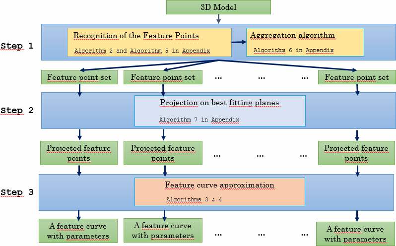
Figure 1: A synthetic flowchart of our method.

In the body of the Main Algorithm 1 the following variables are used: $\mathbb{X}$, which denotes the set of feature points extracted from the model $\mathcal{M}$ by means of the Feature Points Recognition Algorithm 2; $\mathbb{Y}_{j}$, with $j=1\ldots m$, which denotes the subset of points of $\mathbb{X}$ sharing some similar properties obtained applying the Aggregation Algorithm 6; $\mathbb{Z}_{j}$, with $j=1\ldots m$, which is the local projection of $\mathbb{Y}_{j}$ to its best fitting plane obtained applying Projection Algorithm 7; $\mathcal{C}_{j}$, which is the curve of the family $\mathcal{F}$ that best approximates $\mathbb{Z}_{j}$. $\mathcal{C}_{j}$ is obtained applying the Curve Detection Algorithm 4 to $\mathbb{Z}_{j}$ with respect to a family of functions $\mathcal{F}$ in a region $\mathcal{T}$ of the parameter space which is discretized with a step $d$.

3.1 Potential feature points recognition

Using various shape properties (curvatures, parabolic points identification or photometric information) the feature points set is extracted from the input model. In this paper we concentrate on features highlighted by means of curvature functions and/or colorimetric attributes.

The geometric properties are derived using classical curvatures, like minimum, maximum, mean, Gaussian or total curvatures. We denote these well-known geometric quantities by $C_{min}$, $C_{max}$, $C_{mean}$, $C_{Gauss}$, $C_{tot}$ respectively. Several methods for estimating curvatures over triangle meshes and point clouds exist but, unfortunately, there is not a universal solution that works best for every kind of input [70]. We decided to keep our implementation flexible, adopting in alternative a discretization of the normal cycles [15] proposed in the Toolbox graph [55] and the statistic-based method presented in [36].

Input : a 3D model $\mathcal{M}$, the property $prop$ (the type of curvature and/or colour), the threshold $p$ for feature points filtering, an HT-regular family $\mathcal{F}$ of planar curves

Output : a list of curves belonging to the family $\mathcal{F}$

1 begin

       /* extracts the feature points set from the model $\mathcal{M}$ */

2       $\mathbb{X}\leftarrow$ Feature Points Recognition Algorithm 2 applied to $\mathcal{M}$, $prop$ and $p$;

       /* groups the points of $\mathbb{X}$ into smaller dense subsets */

3       $\mathbb{Y}=[\mathbb{Y}_{1},\ldots,\mathbb{Y}_{m}]\leftarrow$ Aggregation Algorithm 6 applied to $\mathbb{X}$;

4       for $j=1,\ldots,m$ do

             /* projects the points of $\mathbb{Y}_{j}$ onto the best fitting plane */

5             $\mathbb{Z}_{j}\leftarrow$Projection Algorithm 7 (see Appendix) applied to $\mathbb{Y}_{j}$;

6             $t\leftarrow$ number of parameters of the curves of $\mathcal{F}$;

             /* initializes the region $\mathcal{T}$ of the parameter space and its discretization step $d$ */

7             $\mathcal{T}\leftarrow[a_{1},b_{1}]\times\ldots\times[a_{t},b_{t}]\in\mathbb{R}^{t}$; $d\leftarrow(d_{1},\ldots,d_{t})\in\mathbb{R}_{>0}^{t}$;

             /* computes the curve of $\mathcal{F}$ that best approximates $\mathbb{Z}_{j}$ */

8             $\mathcal{C}_{j}\leftarrow$ Curve Detection Algorithm 4 applied to $\mathbb{Z}_{j},\mathcal{F},\mathcal{T},d$;

9            

10       end for

11      return $\mathcal{C}=[\mathcal{C}_{1},\ldots,\mathcal{C}_{m}]$

12 end

13

Main Algorithm 1 Feature curve identification for a given 3D model $\mathcal{M}$ with respect to a property (different types of curvatures/colour) and a family $\mathcal{F}$ of curves

The photometric properties can be represented in different colour spaces, such as RGB, HSV, and CIELab spaces. Our choice is to work in the CIELab space [6], which has been proved to approximate human vision in a good way. In such a space, tones and colours are distinct: the $L$ channel is used for the luminosity, which closely matches the human perception of light ($L=0$ yields black and $L=100$ yields diffuse white), whereas the $a$ and $b$ channels specify colours [33].

The different types of curvatures $C_{min}$, $C_{max}$, $C_{mean}$, $C_{Gauss}$, $C_{tot}$, and the luminosity $L$ are used as scalar real functions defined over the surface vertices. One (or more) of these properties is given as input (stored in the variable $prop$) in the Feature Points Recognition Algorithm 2. The feature points $\mathbb{X}$ of the model $\mathcal{M}$ are extracted by selecting the vertices at which the property $prop$ is significant (e.g high maximal curvature and/or low minimal curvature and/or low luminosity). This is automatically achieved by filtering the distribution of the function that we decide to use by means of a filtering threshold $p$ (see Appendix, Algorithm 5). Note that $p$ is given in input in the Main Algorithm 1. Its value varies according to the precision threshold set for the property used to extract the feature points (e.g. in the case of maximum curvature a typical value of $p$ is $80\%$). We sum up the described procedure in the Algorithm 2.

As an illustrative example we show the steps performed by the extraction of the feature points, when applied to a 3D model $\mathcal{M}$ given as a triangulated mesh (made up of approximately $10^{6}$ vertices and $2\cdot 10^{6}$ faces) without photometric properties, see Figure 2(a).

Input : 3D model $\mathcal{M}$, the property $prop$, that is the type of curvature ($C_{min}$, $C_{max}$, $C_{mean}$, $C_{Gauss}$, $C_{tot}$) and/or the $L$ channel, the filtering threshold $p$

Output : Set of feature points $\mathbb{X}\subset\mathbb{R}^{3}$

1

2begin

       /* loads $\mathcal{M}$; faces are optional (available only for meshes) */

3       [vertices, faces]= load($\mathcal{M}$);

       /* evaluates curvatures and colour (if available) */

4      if $prop$ is a curvature then

5             [Cmin, Cmax] = EvaluateCurvatures(vertices, faces);

6             switch $prop$ do

7                   case $C_{mean}$ do Cmean=(Cmin+Cmax)/2;

8                   case $C_{Gauss}$ do CGauss=Cmin.*Cmax;

9                   case $C_{tot}$ do Ctot = abs(Cmin)+ abs(Cmax);

10                  

11             end switch

12            

13      else

14             [L, a, b] = get$\_$Lab($\mathcal{M}$);

15            

16       end if

17      $f\leftarrow$ function according to the property $prop$;

       /* builds the histogram of $f$ and filters it using $p$ */

18       h = histogram(f);

19       v = Filtering(h, p) (see Filtering Algorithm 5 in Appendix);

20      

      /* constructs the feature points set $\mathbb{X}$ */

21       for $j=1\ldots$size(vertices) do

22             if f[j] $>$ v then add vertices[j] to $\mathbb{X}$;

23       end for

      return : $\mathbb{X}$

24      

25 end

26

Feature Points Recognition Algorithm 2 Extracts the feature points sets $\mathbb{X}\subset\mathbb{R}^{3}$ from the input model $\mathcal{M}$

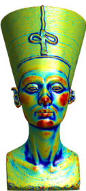
(a)		(b)		(c)
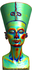
(d)		(e)		(f)

Figure 2: A 3D model $\mathcal{M}$ (a) and the visualization (colours range from blue (low) to red (high)) of the values of different curvatures: (b) minimum curvature, (c) maximum curvature, (d) mean curvature, (e) Gaussian curvature and (f) total curvature.

A visual representation with colours of the different curvature functions computed on the model $\mathcal{M}$ is shown in Figure 2(b)-(f); their histograms are shown in Figure 3. In Figure 4(b) the output of Algorithm 2 when applied to $\mathcal{M}$ using the maximum curvature and filtering the corresponding histogram at $90\%$ is shown.

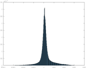
(1) - min curvature		(2) - max curvature		(3) - mean curvature
(4) - Gaussian curvature		(5) - total curvature

Figure 3: Histograms of different curvature functions on the 3D model $\mathcal{M}$ in Figure 2(a)

Once detected, the set $\mathbb{X}$ of feature points is subdivided into smaller clusters (that is, groups of points sharing some similar properties, such as curvature values and/or chromatic attributes) by using classical methods of cluster analysis. Here, we adopt a very well-known density model, the Density-Based Spatial Clustering of Applications with Noise (DBSCAN) method [22], which groups together points that lie closeby marking as outliers isolated points in low-density regions. The DBSCAN algorithm requires two additional parameters: a real positive number $\varepsilon$, the threshold used as the radius of the density region, and a positive integer $MinPoints$, the minimum number of points required to form a dense region. In order to estimate the density of the feature set $\mathbb{X}$ necessary to automatically relate the choice of the threshold $\varepsilon$ to the context, we use the K-Nearest Neighbor (KNN), a very efficient non parametric method that computes the $k$ closest neighbors of a point in a given dataset [24].

We sum up the described procedure in the Appendix (Algorithm 6). Figure 4(c) represents, with different colours, the outcome of the aggregation algorithm when applied to the feature points $\mathbb{X}$ in Figure 4(b).

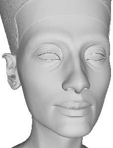
(a)	(b)	(c)

Figure 4: (a) The model $\mathcal{M}$, (b) the feature points $\mathbb{X}$ resulting from Algorithm 2 applied to $\mathcal{M}$ with parameters $prop=2$ and $p=0.9$, and (c) the groups obtained applying Algorithm 6 to $\mathbb{X}$ with parameters $K=50$ and $MinPts=5$.

3.2 Projection of the feature points sets onto best fitting planes

This step performs a local projection of each feature points set to its best fitting plane. This operation does not represent a strong restriction on our method since we apply such a projection separately to each group (obtained from the aggregation of the feature points) and also because we have already assumed that the kind of features that we are looking for can be locally projected onto a plane. Let $\mathbb{Y}$ be a $3$-dimensional set of points that can be injectively projected onto a plane. During this phase the following operations are performed: firstly, the points of the set $\mathbb{Y}$ are shifted to move their centroid onto the origin. Secondly, for the points of $\mathbb{Y}$ a best fitting plane $\Pi$ is found by computing the multiple linear regression using the least squares method. We compute it as follows. We denote by $s$ the cardinality of $\mathbb{Y}$, and we consider the matrix $XY$ of size $s\times 2$ and the column vector $Z$ of size $s\times 1$ whose columns respectively contain the $x$-and $y$-coordinates of the points of $\mathbb{Y}$ and the the $z$-coordinates of the same points. We apply a linear regression function to the pair $(XY,Z)$ and get the real values $b_{1}$ and $b_{2}$ used to construct the best fitting plane $\Pi$, whose equation is $\Pi:z-b_{1}x-b_{2}y=0$. Finally, the orthogonal transformation $\varphi$ moving the plane $\Pi$ onto the plane $z=0$ is defined and applied to the points of $\mathbb{Y}$ to get the new set $\mathbb{Z}$. We sum up the described procedure in the Appendix, Algorithm 7. Figure 5(b) represents the best fitting plane of the subset $\mathbb{Y}_{8}$ depicted in Figure 5(a); the new set $\mathbb{Z}_{8}$ is shown in Figure 5(c).

(a)	(b)	(c)

Figure 5: Representation of (a) the cluster $\mathbb{Y}_{8}$ (see also Figure 4(c)), (b) its best fitting plane $\Pi_{8}$ and the subset $\mathbb{Z}_{8}$ obtained by projecting $\mathbb{Y}_{8}$ onto $\Pi_{8}$.

3.3 Feature curve approximation

Once we have projected every set of points onto its best fitting plane, we apply to the single group elements the generalization of the HT technique (see [10] and [67]) aimed at approximating the feature curve. With respect to the previous application of [10] to images, our approach is novel since we apply the method to each projected 3D feature points set by exploiting a vast catalogue of curves (see Section 4 for a detailed description of the families of curves used in this paper). Further, we propose a method that does not undergo to any grid approximation of the coordinates of the given points.

We provide here some details on the curve detection algorithm which is the core of the HT-based technique. In its classical version [32, 21], HT permits to recover the equation of a straight line exploiting a very easy mathematical principle: starting from points lying on a straight line, defined using the common Cartesian coordinates $x$ and $y$ (or equivalently the polar coordinates $\rho$ and $\theta$) and following the usual slope-intercept parametrization with parameters $a$ and $b$ we end with a collection of straight lines in the parameters’ space (or equivalently sinusoidal curves in the variables $\rho$ and $\theta$) that all intersect in exactly one point. The equation of each straight line is also called Hough transform of the point, usually denoted by $\Gamma_{p}(\mathcal{F})$ (where $\mathcal{F}$ denotes the chosen family of curves, the straight lines in this particular case). The coordinates of the unique intersection point of all the Hough transforms identify the original line.

Following the approach of [9], we consider a collection of curves which includes more complex shapes beyond the commonly used lines, e.g. circles and ellipses (see Section 4). Under the assumption of Hough regularity on the chosen family of curves $\mathcal{F}$ (see [10]), the detection procedure can be detailed as follows. Let $p_{1},\ldots,p_{s}$ be the set of feature points; in the parameter space we find the (unique) intersection of the Hough transforms (the hypersurfaces depending on the parameters) $\Gamma_{p_{1}}(\mathcal{F}),\ldots,\Gamma_{p_{s}}(\mathcal{F})$ corresponding to the points $p_{1},\ldots,p_{s}$; that is, we compute $\lambda=\cap_{i=1\ldots s}\Gamma_{p_{i}}(\mathcal{F})$. Finally, we return the curve of the family $\mathcal{F}$ uniquely determined by the parameter $\lambda$.

From a computational viewpoint, the burden of the outlined methodology is represented by the computation of the intersection of the Hough transforms, which is usually implemented using a so called “voting procedure”. Following [67] the voting procedure can be detailed in the following four steps:

1. Fix a bounded region $\mathcal{T}$ of the parameter space.
   This is achieved exploiting typical characteristics of the chosen family $\mathcal{F}$ of curves, like the bounding box properties or the presence of salient points. In Section 4 we detail how to derive the bounding box of the parameter space from the algebraic or polar representation of various families of curves.

2. Fix a discretization of $\mathcal{T}$.
   This is nontrivial yet fundamental for the detection result which is valid up to the chosen discretization step. The choice of the size of the discretization step is currently done as a percentage of the range interval of each parameter. For some recent results on this topic we refer to [68]. Let $\mathcal{T}=[a_{1},b_{1}]\times\ldots\times[a_{t},b_{t}]$ be the fixed region of the parameters space and $d=(d_{1},\ldots,d_{t})\in\mathbb{R}_{>0}^{t}$ be the discretization step. For each $k=1,\ldots,t$, we define

   $$J_{k}:=\left\lceil\frac{b_{k}-a_{k}-\frac{d_{k}}{2}}{d_{k}}\right\rceil+1,$$ (1)

   where $\lceil x\rceil=\min\{z\in\mathbb{N}\>|\>z\geq x\}$ and

   $$\lambda_{k,j_{k}}:=a_{k}+j_{k}d_{k}$$ (2)

   with $j_{k}=0,\ldots,J_{k}-1$. Here $J_{k}$ denotes the number of considered samples for each component, and $j_{k}$ the index of the sample. We denote by ${\bf j}$ the multi-index $(j_{1},\ldots,j_{t})$, by ${\lambda}_{\bf j}:=(\lambda_{1,j_{1}},\ldots,\lambda_{t,j_{t}})$ the ${\bf j}$-th sampling point, and by

   $${\bf C}({\bf j}):=\left\{(\lambda_{1},\ldots,\lambda_{t})\in\mathbb{R}^{t}\;\Big{|}\;\lambda_{k}\in\left[\lambda_{k,j_{k}}-\frac{d_{k}}{2},\lambda_{k,j_{k}}+\frac{d_{k}}{2}\right),\;k=1,\ldots,t\right\}$$ (3)

   the cell centered at (and represented by) the point ${\lambda}_{\bf j}$. The discretization of $\mathcal{T}$ is given by the $J_{1}\times\cdots\times J_{n}$ cells of type ${\bf C}({\bf j})$ which are a covering of the region $\mathcal{T}$.

3. Construct an accumulator function $\mathcal{A}:\mathcal{T}\rightarrow\mathbb{N}$, which is defined as $\mathcal{A}=\sum_{1=1\ldots s}f_{p_{i}}$ where $f_{p_{i}}:\mathcal{T}\rightarrow\mathbb{N}$ is defined as follows:

   $$f_{p_{i}}(c)=\left\{\begin{array}[]{ll}1&\mbox{if the Hough Transform }\Gamma_{p_{i}}(\mathcal{F})\ \mbox{crosses the cell}\ c;\\ 0&\mbox{otherwise}.\end{array}\right.$$

   For the evaluation of each $f_{p_{i}}$ we adopt the Crossing Cell algorithm (detailed in Algorithm 3) which is based on bounds of the evaluation of $f_{p_{i}}$ theoretically proved in [67]. The function $EvalFirstBound$, resp. $EvalSecondBound$, in the pseudocode represents the evaluation of the bound $B_{1}$ (resp. $B_{2}$) of a given polynomial $f$ in $n$ variables w.r.t a cell centered at $p$ with radius $\varepsilon$. Such bounds depend on the Jacobian and the Hessian matrices of $f$, denoted by ${\rm Jac}_{f}$ and $H_{f}$ respectively. They are defined as follows:

   $$B_{1} = \|{\rm Jac}_{f}(p)^{t}\|_{1}\varepsilon+\frac{n}{2}H\varepsilon^{2}$$ (4)

   $$B_{2} = \frac{2R}{{\rm J}(c+n^{5/2}H{\rm J}R)}$$ (5)

   where $H=\max_{\{x\in\mathbb{R}^{n}:\|x-p\|_{\infty}\leq\varepsilon\}}\|H_{f}(x)\|_{\infty}$, $R<\min\Big{\{}\varepsilon,\frac{\|{\rm Jac}_{f}(p)\|_{1}}{H}\Big{\}}$, $c=\max\{2,\sqrt{n}\}$ and ${\rm J}=\sup_{\{x\in\mathbb{R}^{n}:\|x-p\|_{\infty}<R\}}\|{\rm Jac}_{f}^{\dagger}(x)\|_{\infty}$, with ${\rm Jac}_{f}^{\dagger}$ denoting the Moore-Penrose pseudo-inverse of ${\rm Jac}_{f}$. Since the above quantities depend on the Jacobian and the Hessian matrices, $p$ must be a point for which these values are non-trivial. Note that the evaluation is made over a symbolic representation of the Jacobian matrix, its pseudo-inverse and the Hessian matrix. This implies that the computational cost of this operation is constant while their symbolic representation is computed only once, in the overall Curve Detection Algorithm 4. In our implementation we use the system CoCoA [5] for the symbolic manipulation of polynomials and matrices.

4. Identify the cell corresponding to the maximum value of the accumulator function and return the coordinates of its center.
   Following the general theory, the HT regularity guarantees that the maximum of the accumulator function is unique. In addition, being based on local maxima, the voting strategy permits to identify curves also from partial and incomplete data, even if the missing part is significant, see the examples in Figure 19(I.c-d) and in Figure 19(II.c-d).

Input : The symbolic representation of $f$ in the variables $x_{1},\ldots,x_{n}$, a point $p\in\mathbb{R}^{n}$, a tolerance $\varepsilon$, the symbolic expression of the Jacobian ${\rm Jac}_{f}$ of $f$, the Moore-Penrose pseudo-inverse ${\rm Jac}_{f}^{\dagger}$ of ${\rm Jac}_{f}$, and the Hessian matrix $H_{f}$ of $f$.

Output : an element of $\{0,1$, undetermined$\}$

1

2begin

3       $B_{1}\leftarrow EvalFirstBound(f,p,\varepsilon,{\rm Jac}_{f})$ (see formula (4));

4       $B_{2}\leftarrow EvalSecondBound(f,p,\varepsilon,{\rm Jac}_{f}^{\dagger},H_{f})$ (see formula (5));

5       if $abs(f(p))>B_{1}$ then

6            returnValue=0

7      else

8             if $abs(f(p))<B_{2}$ then returnValue=1

9             else returnValue= undetermined end

10       end if

      return : returnValue

11      

12 end

13

Crossing Cell Algorithm 3 Returns $1$ or $0$ if $f=0$ crosses or not the cell of radius $\varepsilon$ centered at $p$. If not decidable it returns undetermined.

The Curve Detection Algorithm 4 sums up the curve detection’s procedure described in the previous steps $1$-$4$. Note that a prototype implementation in CoCoA of the Curve Detection Algorithm 4 is freely available.

To give an idea of the outcome of the Algorithm 4, we have run it on the set $\mathbb{Z}_{8}$ (represented in Figure 5(c)) made of $981$ points. In this example we use the geometric petal curve, an HT-regular family of curves presented both in polar and in cartesian form, see Section 4 for details. By exploiting the bounding box of the set $\mathbb{Z}_{8}$ and properties of the geometric petal curve, we consider $\mathcal{T}=[121,122]\times[0.43,0.45]$ and $d=(0.025,0.005)$. The Algorithm 4 applied to this framework computes the geometric petal curve depicted in Figure 6(a); the feature curve is shown on the 3D model as the red line in Figure 6(b).

Input : A finite set $\mathbb{X}=\{p_{1},\ldots,p_{s}\}\subset\mathbb{R}^{2}$, an HT-regular family $\mathcal{F}=F(x,y,\lambda_{1}1,\ldots,\lambda_{t})$ of curves, a region $\mathcal{T}=[a_{1},b_{1}]\times\ldots\times[a_{t},b_{t}]\subset\mathbb{R}^{t}$ of the parameter space, a discretizaton step $d=(d_{1},\ldots,d_{t})\in\mathbb{R}_{>0}^{t}$

Output : a curve $\mathcal{C}$ of the family $\mathcal{F}$

1

2begin

       /* discretizes the region $\mathcal{T}$ with step $d$ */

3       Initialize $J_{k}$, with $k=1,\ldots t$, (see formula (1));

4       Initialize $\lambda_{k,j_{k}}$, with $k=1,\ldots t$ and $j_{k}=0,\ldots,J_{k}-1$ (see formula (2));

5       Initialize $\lambda_{\textrm{\bf j}}$ and $C(\textrm{\bf j})$, with $\textrm{\bf j}\in J_{1}\times\ldots\times J_{t}$ (see formula (3));

       /* constructs of the multi-matrix $\mathcal{A}$ */

6       $\mathcal{A}\leftarrow$ zero matrix of size $J_{1}\times\ldots\times J_{t}$;

7       $Jac\leftarrow$ Jacobian matrix of $F(x,y,\lambda_{1},\ldots,\lambda_{t})$ w.r.t $\lambda_{1},\ldots,\lambda_{t}$;

8       ${\rm Jac}_{f}^{\dagger}\leftarrow$ Moore-Penrose pseudo-inverse of $Jac$;

9       $H_{f}\leftarrow$ Hessian matrix of $F(x,y,\lambda_{1},\ldots,\lambda_{t})$ w.r.t $\lambda_{1},\ldots,\lambda_{t}$;

10       for $i=1,\ldots,s$ do

11             for each $\textrm{\bf{j}}\in J_{1}\times\ldots\times J_{t}$ do

12                   $\mathcal{A}(\textrm{\bf{j}})\leftarrow\mathcal{A}(\textrm{\bf{j}})+\textrm{Crossing Cell}(F(p_{i}),\lambda_{\textrm{\bf{j}}},\frac{d}{2},{\rm Jac}_{f}(p_{i}),{\rm Jac}_{f}^{\dagger}(p_{i}),H_{f}(p_{i}))$ (Alg. 3)

13             end for

14            

15       end for

      /* computation of the maximum of $\mathcal{A}$ */

16       ${\bf\bar{j}}\leftarrow\max(\mathcal{A}$);

17       return $\mathcal{C}=\mathcal{C}(\lambda_{\bf\bar{j}})$, the curve of $\mathcal{F}$ with parameters $\lambda_{\bf\bar{j}}$

18 end

19

Curve Detection Algorithm 4 Computes the curve $\mathcal{C}$ of the family $\mathcal{F}$ best detecting the profile highlighted by the points of the set $\mathbb{X}$

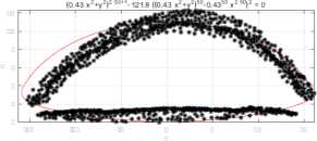
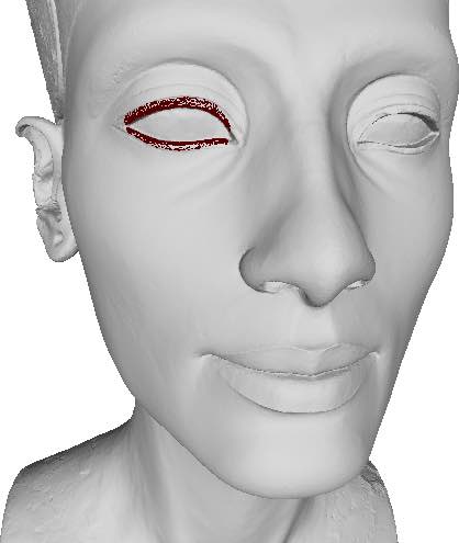
(a)		(b)

Figure 6: Representation of the set $\mathbb{Z}_{8}$ and the geometric petal curve (in red) computed by Algorithm 4 (a) and visualization of the curve (in red) on the original model of Figure 2(b).

We outline the steps of the Main Algorithm 1 when applied to the $3D$ model (made up of $152850$ vertices and $305695$ faces) represented in Figure 7(a). In this case, in order to detect the spiral-like curves we work with the generalized family $\mathcal{F}$ of Archimedean spirals (see Section 4 for more details). The Feature Points Recogniton Algorithm 2 is applied using the mean curvature and returns a set $\mathbb{X}$ made up of $12689$ points. Then, the Aggregation Algorithm 6 (in Appendix) subdivides the points of $\mathbb{X}$ into $8$ groups $\mathbb{Y}_{1},\ldots,\mathbb{Y}_{8}$. For shortness, we give details for the first group, $\mathbb{Y}_{1}$, which is made up of $2382$ points. Exploiting some geometrical properties of the Archimedean spirals (see again Section 4), we fix and discretize a suitable region of the parameter space, and apply the Curve Detection Algorithm 4. The corresponding spiral curve is depicted in Figure 7(b) and shown on the 3D model as the red line in Figure 7(c-d). Other detected spirals are marked using different colours in Figure 7(c-d).

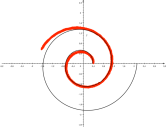
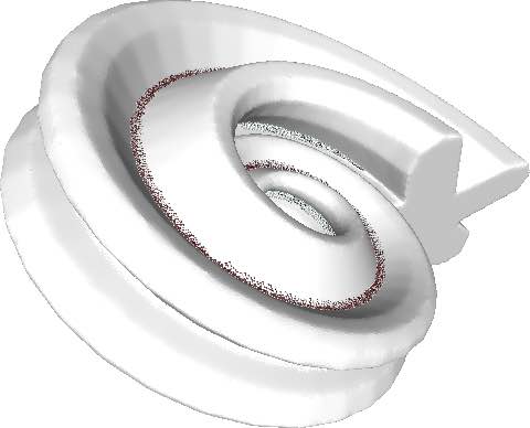
(a)		(b)		(c)		(d)

Figure 7: A 3D model (a), recognition of a spiral (b), two views of the spiral-like curves detected by our method (c,d).

3.4 Computational complexity

Here we briefly analyse the computational complexity of the method. The feature points recognition function (Algorithm 2) depends on the chosen procedure, in case we adopt the curvature estimation proposed in [15] the computational complexity is $O(n\log n)$, where $n$ represents the number of points of the model. The computational cost for converting RGB coordinates into CIELab ones is linear ($O(n)$). Denoting $n_{f}$ the number of the feature points (in general $n_{f}\ll n$), the aggregation into groups using DBSCAN (see the Algorithm 6 in the Appendix) takes $O(n{{}_{f}}^{2})$ operations in the worst case [22] (on average it takes $O(n_{f}\log n_{f})$ operations, and thus it is overcome by the KNN search operation detailed in the Algorithm 6 that costs $O(kn_{f}\log n_{f})$, see [25].

After the aggregation of the feature points, the projection (Algorithm 7 in the Appendix) and the curve detection (Algorithm 4) algorithms are applied to each group, separately (note that the sum $s_{f}$ of the elements in the groups is, in general, smaller than $n_{f}$ because of the presence of outliers and small groups).

The cost of the curve detection algorithm is dominated by the size of the discretization of the region $\mathcal{T}$, as detailed in the Algorithm 4. Such a discretization consists of $M=\prod_{k=1}^{t}J_{k}$ elements, where $t$ is the number of parameters (in the curves proposed in this paper, $t=2,3$) and $J_{k}$ is the number of subdivisions for the $k$th parameter, see formula (1). The evaluation of the HT on each cell is constant and the Jacobian, pseudo-inverse and Hessian matrices are symbolically computed once for each curve; therefore, the cost of fitting a curve to each group with our HT method is $O(M)$. Since the curve fitting is repeated for $m$ groups, the overall cost of our method is $O(\max(n\log n,ms{{}_{f}}^{2},mM))$ where $n$, $m$, $s_{f}$ and $M$ represent, respectively, the number of points of the 3D model, the number of groups of feature points and their maximum size, the size of the discrete space on which we evaluate the accumulator function.

4 Families of curves

In this section we list the families of curves used in our experiments, focusing in each case on their main properties and characteristics (parameter dependency, boundedness, computation of the bounding box). For every family of curves we explicitly describe how to derive from its algebraic representation the parameters used as input for the Curve Detection Algorithm 4. The selected curves form an atlas, which is both flexible and open: in fact, these curves are modifiable (for instance, by adding, stretching or scaling parameters) and the insertion of new families of curves is always possible. Note that the atlas comprises families of curves defined using Cartesian or polar coordinates, since our framework works on both cases.

Our collection also includes some elementary, but likewise interesting, families of algebraic curves like straight lines, circles and ellipses, which can be exploited to detect for instance eyes contours, pupils shapes and lips lines. Their equation are linear (straight lines) and quadratic (ellipses and circles) and depend on $3$ parameters at most.

In the following, we list the other families of the collection; these curves mainly come from [61] that contains a rich vocabulary of curves many of which are suitable for our approach, too. The curves employed in our experiments (see Section 5) are: the curve of Lamet, the citrus curve, the Archimedean spiral, the curve with $m$-convexities and the geometric petal curve.

The curve of Lamet is a curve of degree $m$, with $m$ an even positive integer, whose outline is a rectangle with rounded corners. Its Cartesian equation is:

$$\frac{x^{m}}{a^{m}}+\frac{y^{m}}{b}=1$$

or equivalently in polynomial form: $bx^{m}+a^{m}y^{m}=a^{m}b$, with $a,b\in\mathbb{R}_{>0}$ and it is a bounded connected closed curve with two axes of symmetry (the $x$ and the $y$ axes). The curve of Lamet is contained in the rectangular region $[-a,a]\times[-b^{1/m},b^{1/m}]$. Some examples are provided in Figure 8 using different values of the parameters $a$, $b$ and $m$.

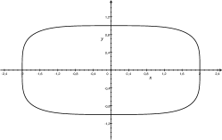
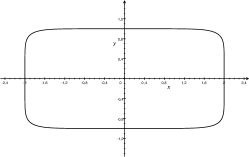
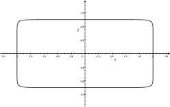
(a)	(b)	(c)

Figure 8: Curve of Lamet with $a=2$, $b=1$ and: (a) $m=4$, (b) $m=8$, and (c) $m=16$.

Another interesting shape (for instance when looking for a mouth, an eye feature or a leaf like decoration) is given by the sextic surface of equation

$$a^{4}(x^{2}+z^{2})+(y-a)^{3}y^{2}=0$$

with $a\in\mathbb{R}$, called the zitrus (or citrus) surface by Herwig Hauser [1]. The citrus surface has bounding box $[-\frac{a}{8},\frac{a}{8}]\times[0,a]\times[-\frac{a}{8},\frac{a}{8}]$, centroid at $(0,\frac{a}{2},0)$ and volume $\frac{1}{140}\pi a^{3}$.

We derive the citrus curve of equation $f_{a}(x,y)=0$ as the intersection of a rotation of $\pi/2$ of the citrus surface with the plane $z=0$, where $f_{a}(x,y)$ is the following sextic polynomial

$$f_{a}(x,y)=a^{4}y^{2}+\left(x-\frac{a}{2}\right)^{3}\left(x+\frac{a}{2}\right)^{3}$$

with $a\in\mathbb{R}$ (see Figure 9(a)). The citrus curve is a symmetric bounded curve with bounding box $[-\frac{a}{2},\frac{a}{2}]\times[-\frac{a}{8},\frac{a}{8}]$.

To include shapes with a different ratio, we introduce another citrus curve whose equation is $f_{a,c}(x,y)=0$ (which is simply stretched or shortened along the $y$-axis) where $f_{a,c}(x,y)$ is given by:

$$f(x,y)=a^{4}c^{2}y^{2}+\left(x-\frac{a}{2}\right)^{3}\left(x+\frac{a}{2}\right)^{3}$$

with $a,c\in\mathbb{R}$ (see Figure 9(b)). Note that this is again a symmetric bounded curve with bounding box $[-\frac{a}{2},\frac{a}{2}]\times[-\frac{a}{8c},\frac{a}{8c}]$.

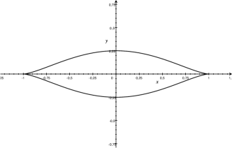
(a)		(b)

Figure 9: The citrus curve of equation: (a) $f_{a}(x,y)=0$ with $a=2$, $c=1/4$, (b) $f_{a,c}(x,y)=0$ with $a=2$, $c=1/2$.

The Archimedean spiral (or arithmetic spiral) can be found in human artefact decorations as well as in nature. Its polar equation is:

$$\rho=a+b\theta$$

with $a,b\in\mathbb{R}$. The Archimedean spiral is an unbounded connected curve with a single singular point (the cessation point $(a,0)$). Two consecutive turnings of the spiral have a constant separation distance equal to $2\pi b$, hence the name arithmetic spiral. Another peculiar aspect is that, though its unboundedness nature, the $k$th turning of the spiral is contained in a region bounded by two concentric circles of radii $a+2(k-1)\pi b$ and $a+2k\pi b$. In particular, the first turning is contained in the circular annulus of radii $a$ and $a+2\pi b$. An example is provided in Figure 10(a).

We extend the Archimedean spiral by weakening its constant pitch property, introducing an extra parameter $c$; its polar equation becomes:

$$\rho=a+b\theta+c\theta^{2}$$

with $a,b,c\in\mathbb{R}$. Analogously to the Archimedean spiral, this generalized family is still an unbounded connected curve with a single singular point (the cessation point $(a,0)$). An example is provided in Figure 10(b).

In order to show the behaviour of the Main Algorithm 1, the generalized version of the Archimedean spirals has been employed in Section 3. Some computational details have been provided in the case of the set $\mathbb{Y}_{1}$, represented in Figure 7(b). Exploiting the Cartesian coordinates of the cessation point $(0.3915,0.0048)$ of the set $\mathbb{Y}_{1}$, and the fact that the first turning of the spiral is contained in the circumference of radius $1.1542$ centered at the origin, we considered the region of the parameter space $T=[0.35,0.45]\times[0.1,0.15]\times[0.0032,0.0048]$ and the discretization step $(0.01,0.01,0.004)$. Figure 7 presents a set of feature curves recognized with the extended Archimedean spiral. With reference to the example shown in Figure 7(b), the maximum of the accumulator function is $44$ (the second maximum has value $29$) and corresponds to the cell with center $(\frac{7}{20},\frac{1}{10},\frac{2}{625})$.

(a)		(b)

Figure 10: Archimedean spirals with parameters: (a) $a=1/10$, $b=1/2\pi$ and (b) $a=1/10$, $b=1/2\pi$, $c=1/100$.

Figure 11 shows another family of curves. The curve with $m$-convexities defined by the polar equation

$$\rho=\frac{a}{1+b\cos(m\theta)}$$

with $a,b\in\mathbb{R}_{>0}$, $b<1$, and $m\in\mathbb{N_{+}}$, $m\geq 2$. The curve with $m$-convexities is a bounded connected closed curve with $m$ axes of symmetry (the straight lines of equation $x\sin\frac{\pi}{m}k-y\cos\frac{\pi}{m}k=0$, with $k=0,\ldots,m-1$). This curve is contained in a region bounded by two concentric circles of radii $\frac{a}{1+b}$ and $\frac{a}{1-b}$. The shape of the curve with $m$-convexities strongly depends on the values of its parameters. In particular, the parameter $a$ plays the role of a scale factor, while the values of $b$ tune the convexities’ sharpness. Some examples of curves with $m$-convexities are provided in Figure 11 where in the first row parameter $m=3$, and in the second row parameter $m=5$.

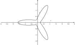
(a)	(b)	(c)
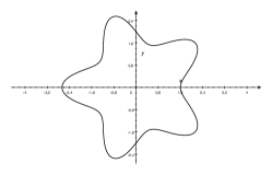
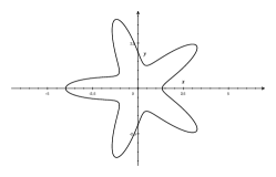
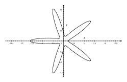
(d)	(e)	(f)

Figure 11: Curves with $m$-convexities with $a=2$ and (a) $b=1/4$, $m=3$, (b) $b=1/2$, $m=3$, (c) $b=3/4$, $m=3$, (d) $b=1/4$, $m=5$, (e) $b=1/2$, $m=5$, (f) $b=3/4$, $m=5$.

The so-called geometric petal curve resembles an eye contour line, for particular values of the parameters. Its polar equation is:

$$\rho=a+b\cos^{2n}\theta$$

with $n\in\mathbb{N}_{+}$ and $a,b\in\mathbb{R}$. The geometrical petal is a bounded symmetric curve with a singularity at the origin. Some examples are provided in Figure 12(a)-(b) where the values of the parameters are set as follows: $a=2$, $b=-2$ and $n=1,10$.

For our purposes, we can restrict to the case $b=-a$. In this case, we observe that the curve is completely contained inside the circle of radius $\sqrt{2}a$. We pass to the Cartesian equation using the standard substitutions $\rho=\sqrt{x^{2}+y^{2}}$ and $\cos\theta=x/\sqrt{x^{2}+y^{2}}$; further, in order to lower the parameters degree, we replace $a$ by $\sqrt{a}$. The Cartesian equation of the geometric petal is $g_{a}(x,y)=0$ where

$$g_{a}(x,y)=(x^{2}+y^{2})^{2n+1}-a[(x^{2}+y^{2})^{n}-x^{2n}]^{2}$$

From an analytic intersection of the curve with the Cartesian axes, we compute the bounding box of the curve as: $\left[-\frac{2n}{2n+1}\sqrt{a}\sqrt[2n]{\frac{1}{2n+1}},\frac{2n}{2n+1}\sqrt{a}\sqrt[2n]{\frac{1}{2n+1}}\right]\times\left[-\sqrt{a},\sqrt{a}\right]$.

Most of times, like in the extraction/localization of eyes contours, we need a shape which is more stretched along the $x$-axis (see Figure 12(c)-(d)). We stretch the geometric petal by scaling the $x$-variable by a factor of $\sqrt{c}$, where $c\in\mathbb{R}_{>0}$. The new Cartesian equation of the curve is $g_{a,c}(x,y)=0$ where

$$g_{a,c}(x,y)=(cx^{2}+y^{2})^{2n+1}-a[(cx^{2}+y^{2})^{n}-c^{n}x^{2n}]^{2}.$$ (6)

with bounding box $\left[-\frac{2n}{2n+1}\sqrt{\frac{a}{c}}\sqrt[2n]{\frac{1}{2n+1}},\frac{2n}{2n+1}\sqrt{\frac{a}{c}}\sqrt[2n]{\frac{1}{2n+1}}\right]\times\left[-\sqrt{a},\sqrt{a}\right]$.

To give an idea of the outcome of Algorithm 4, the stretched version of the geometric petal curve (equation 6) has been employed in Section 3. In that example, we fixed $n=50$ (indeed the shape of the geometric petal curve changes with this parameter, see again Figure 12) and, exploiting the bounding box of the set $\mathbb{Z}_{8}$ (see Figure 5(c)), we considered a region $\mathcal{T}=[121,122]\times[0.43,0.45]$ of the parameter space.

In the following, we show how to reduce the number of parameters of this curve. We observed that the value of the exponent parameter $n$ is related to the bounding box of the curve; indeed it has to satisfy the following condition:

$$\frac{2n}{2n+1}\left(1-\sqrt[n]{\frac{1}{2n+1}}\right)^{1/2}=\frac{y_{B}}{y_{A}}$$

where $y_{A}$ and $y_{B}$ are the $y$-coordinates values of the points $A$ and $B$ (see Figure 12 (c)-(d)). By using the previous relation, it is possible to estimate the value of $n$, thus working with a curve which depends on the two parameters $a$ and $c$.

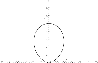
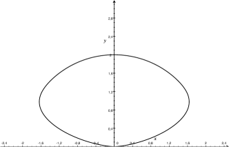
(a)		(b)
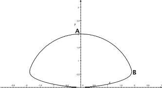
(c)		(d)

Figure 12: Geometric petal curves with parameters $a=2$, $b=-2$ and (a) $n=1$, (b) $n=10$. Geometric petal curves defined by $g_{a,c}(x,y)=0$ with parameters $a=4$, $n=50$ and (c) $c=1$, (d) $c=1/2$.

4.1 Compound curves

To grasp compound shapes we use more families of curves simultaneously. We represent compound curves as a combination of different families of curves and define their equation simply as the product of (two or more) curves’ equations. In the following we show some examples of possible compositions.

Combining a citrus curve and a circle we get the new family of curves of equation:

$$\left(a^{4}y^{2}+\left(x-\frac{a}{2}\right)^{3}\left(x+\frac{a}{2}\right)^{3}\right)\left(x^{2}+y^{2}-\frac{a^{2}}{64}\right)=0$$

with $a\in\mathbb{R}_{>}0$. An example is provided in Figure 13(a) where the parameter is $a=2$.

Another possibility is to couple a citrus curve with a line (we choose one of the two axes of symmetry, for instance the $x$ axis) whose equation is:

$$y\left(a^{4}y^{2}+\left(x-\frac{a}{2}\right)^{3}\left(x+\frac{a}{2}\right)^{3}\right)=0$$

with $a\in\mathbb{R}_{>}0$. An example is provided in Figure 13(b) where the parameter is $a=2$. An application of the use of this compound curve is given in Figure 17(b).

It is also possible to associate a curve with $5$-convexities with a circumference; the resulting polar equation is:

$$\left(\rho-\frac{a}{1+b\cos(5\theta)}\right)(\rho-r)=0$$

with $a,b,r\in\mathbb{R}_{>0}$, $b<1$ and $r\leq\frac{a}{1+b}$. An example is provided in Figure 13(c).

Finally, starting with three ellipses we construct a family of algebraic whose equation is:

$$\left(\frac{x^{2}}{a^{2}}+\frac{y^{2}}{b^{2}}-1\right)\left(\frac{16x^{2}}{9a^{2}}+\frac{(2y-b)^{2}}{b^{2}}-1\right)\left(\frac{4x^{2}}{b^{2}}+\frac{y^{2}}{b^{2}}-1\right)=0$$

with $a,b\in\mathbb{R}_{>0}$. An example is provided in Figure 13(d).

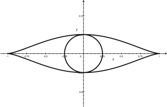
(a)		(b)
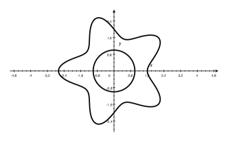
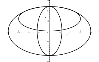
(c)		(d)

Figure 13: Compound curves: (a) citrus curve with $a=2$ coupled with a circumference; (b) citrus curve with $a=2$ coupled with the line $y=0$; (c) curve with $5$-convexities coupled with a circumference with $a=2$, $b=1/4$, $r=1$; (d) three ellipses with $a=10$, $b=6$.

5 Examples and conclusive remarks

Our method has been tested on a collection of artefacts and models collected from the web, the AIM@SHAPE repository [3], the STARC repository [2] and the 3D dataset of the EPSRC project [4].

Most of the models are triangulated meshes; an exception is represented by the model in Figure 19(I.a), which is given as a point cloud. Further, in the examples in Figure 16(IV.a) and 19(I.a) the colorimetric information is available and combined with the curvature; in the models in Figure 15(IV.a) and Figure 18(II.a) features are only characterized by the dark colour of the decoration; the other models come without any colorimetric information and we adopt the maximum, minimum and mean curvature properties. In all the examples, the model embedding in the $3$-dimensional space is completely random and the “best” view shown in the pictures is artificially reported for the user’s convenience. Furthermore, the features we identify are view-independent and represented by curves that can be locally projected onto a plane without any overlap.

For the feature identification, we assume to know in advance the class of features that are present in an object (for instance because there exists an archeological description of the artwork), thus converting the problem into a recognition of definite curves that identifies specific parts such as mouth, eyes, pupils, decorations, buttons, etc. on that model. Once aggregated and projected onto a plane, each single feature group of points is fitted with a potential feature curve and the value of the HT aggregation function is kept as the voting for that. After all curves are run, we keep the highest vote to select the curve that better fits with that feature. Sometimes more than one curve potentially fits the feature point set; in this case we have selected the curve with the highest value of the HT aggregation function.

Figure 14 presents an overview of multiple feature curves obtained by our method. These examples are shown in a portion of the model but are valid for all the instances of the same features. Multiple instances of the same family are shown in Figure 14(I) and Figure 14(II), in which the curves are circles with different radii, in Figure 14(III) and Figure 14(IV), where the detected curves belong to the family of curves with $5$-convexities, in Figure 14(V) and Figure 14(VI), where different Archimedean spirals have been used.

I.
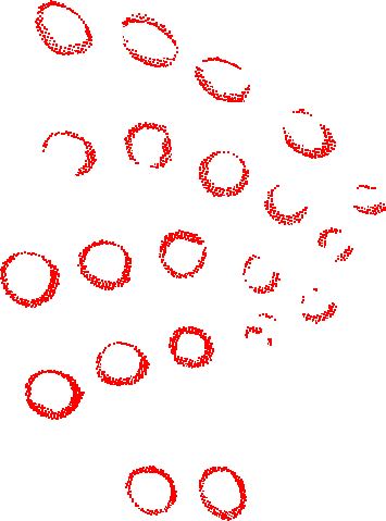
		(a)		(b)		(c)
II.
		(a)		(b)		(c)
III.
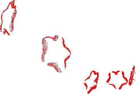
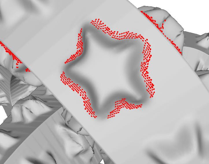
		(a)		(b)		(c)
IV.
		(a)		(b)		(c)
V.
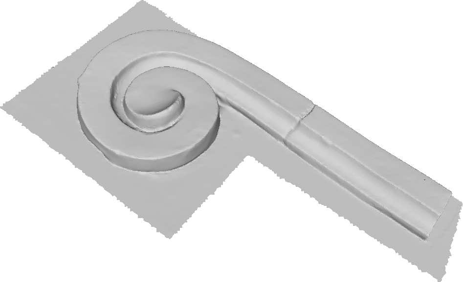
		(a)		(b)		(c)
VI.
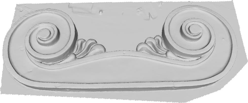
		(a)		(b)		(c)

Figure 14: Examples of recognition of various feature curves; I. circles on the Gargoyle model (the AIM@SHAPE repository [3]); circles on a tentacle of an octopus model; III. stars (curves with $5$-convexities) on the knot model (the AIM@SHAPE repository [3]); IV. stars (curves with $5$-convexities) of different sizes on the trim-star model (the AIM@SHAPE repository [3]); V. and VI. spirals on architectural ornamental artefacts (from the 3D dataset of the EPSRC project [4]).

It is also possible to recognize different families of curves on the same surface, as it happens in the models in Figure 15(I), where circles are combined with two curves of Lamet, in Figure 15(II), where a curve with $5$-convexities is used in combination with a circle, in Figure 15(III), where a curve with $8$-convexities is contained in a region delimited by two concentric circles, and in Figure 15(IV), where the decoration is a repeated pattern of leaves, each one identified with a specific group and approximated by a citrus or a geometric petal curve.

I.
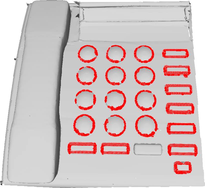
		(a)		(b)		(c)
II.
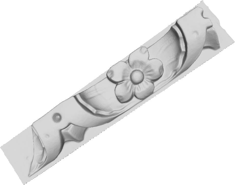
		(a)		(b)		(c)
III.
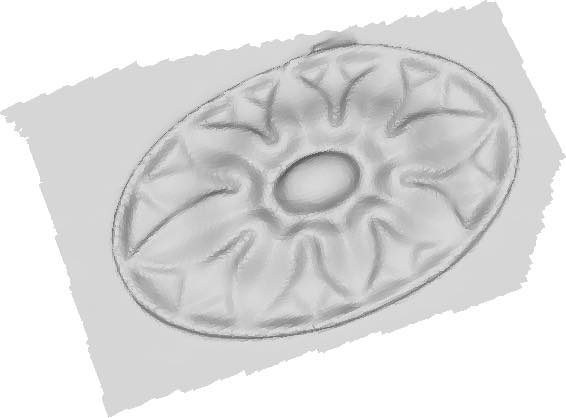
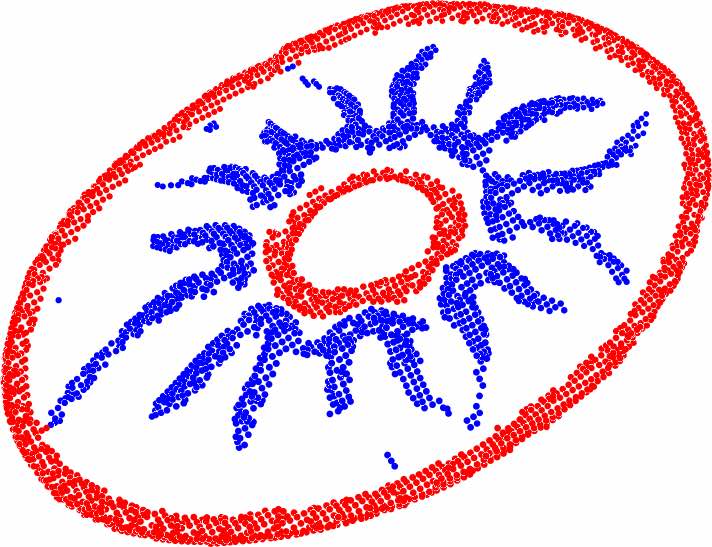
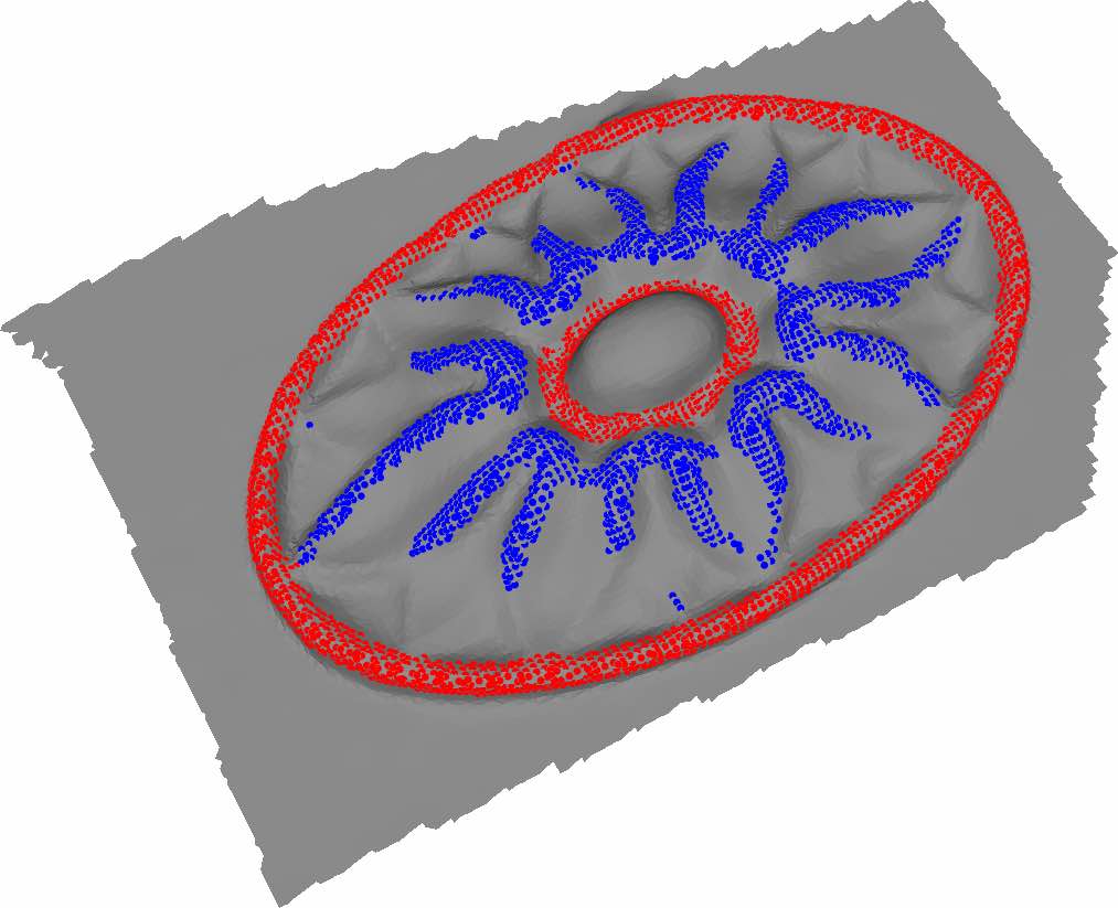
		(a)		(b)		(c)
IV.
		(a)		(b)		(c)

Figure 15: I. circles and curves of Lamet on a phone model; II. a circle and a curve with $5$-convexities on an architectural ornamental artefact (from the 3D dataset of the EPSRC project [4]); III. a curve with $8$-convexities contained in a region delimited by two concentric circles on an architectural ornamental artefact (from the 3D dataset of the EPSRC project [4]); IV. decorations on a bust (from the STARC repository [2]).

Figure 16 shows four examples of eye contours detection from 3D models. The eyes in the first row are better approximated by the citrus curve while in the other three cases the geometric petal is the best fitting curve.

I.
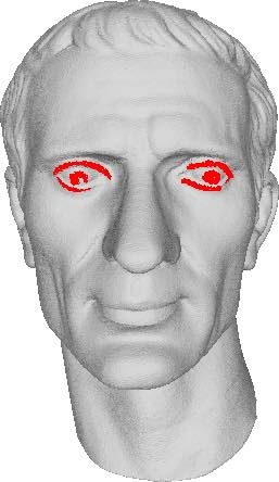
	(a)	(b)	(c)	(d)
II.
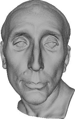
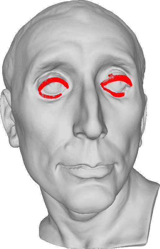
	(a)	(b)	(c)	(d)
III.
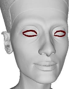
	(a)	(b)	(c)	(d)
IV.
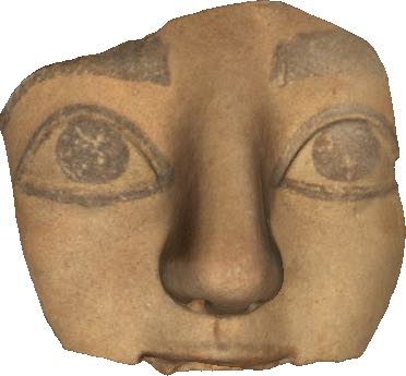
	(a)	(b)	(c)	(d)

Figure 16: Detection of eye contours and pupils on collection of artefacts collected from the AIM@SHAPE repository [3] and the STARC repository [2].

The automatic detection of multiple instances of the same family of curves, possibly with parameter changes as in the case of circles of different radii (e.g. the suction cups of the octopus model, see again Figure 14.II), is automatically done in the space of the parameters by the HT procedure. As a side effect, this immediately yields the equation of the curve that represents these feature points.

An important advantage of our approach is the flexible choice of the family of algebraic curves used to approximate the desired features, thus being adaptive to approximate various shapes. Our set of primitives includes generic algebraic curves and it can be extended to all curves with an implicit representation, see Section 4.

As discussed in Section 4.1, another interesting point is the possibility of recognizing compound features as a whole, as for the eye contour and the pupil, see examples in Figures 16.I and 17(a). Figure 17(b) detects a mouth contour combining a citrus curve with a line. Such an option opens the method to a wide range of curves that includes also repeated patterns like bundles of straight lines or quite complex decorations, see examples in Figure 15.

Another major benefit of using an HT-based method is the HT well known robustness to noise and outliers. Moreover, by selecting the curve with the highest score of the HT aggregation function, our method is able to keep a good recognition power also in the case of degraded (Figure 18) and partial features (Figure 19). Moreover, we are able to work on both 3D meshes and point clouds, thus paving the road to the application of the method to object completion and model repairing.

In addition, it is important to point out that we can similarly parametrize features that are comparable. As we extract a feature curve and its parameters, we can use them to build a template useful for searching similar features in the artefacts, even if heavily incomplete, see Figure 18(II.c-d) and Figure 19(I.c-d) and Figure 19(II.c-d).

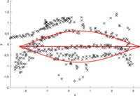
(a)		(b)

Figure 17: Combined anatomical shapes: (a) a circumference and a geometric petal curve detecting an eye; (b) a citrus curve with a line detecting a mouth.

I.
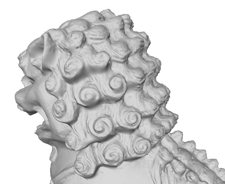
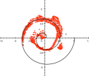
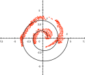
	(a)	(b)	(c)	(d)
II.
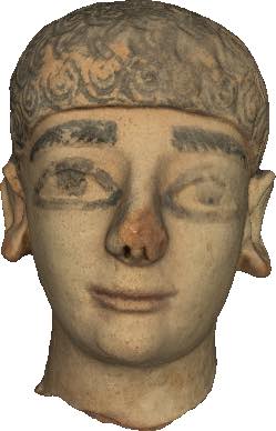
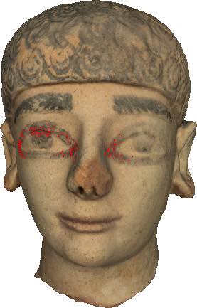
	(a)	(b)	(c)	(d)

Figure 18: Feature recognition on models with degraded features.

I.
		(a)	(b)	(c)	(d)
II.
		(a)	(b)	(c)	(d)

Figure 19: Feature recognition on models (from the STARC repository [2]) with partial features.

(a)		(b)

Figure 20: Colours represent different parameters of the HT.

With reference to Figure 20, we use different colours to show the feature curves identified by different curves/parameters. In Figure 20(a), the blue lines represent the circles, all with the same radius, while the red and green lines depict the curves of Lamet. In particular, the red and the green lines are used for Lamet curves which differ for the values of the parameters $a$ and $b$. Similarly, in Figure 20(b) which represents a tentacle of an octopus model, the red graduate shadings are used to highlight the different radii of the detected circles.

Different colours are also used in Figure 21 where two concentric spirals (red and blue) with different parameters, are detected. Because of the proximity of the two features curves and the presence of degradation and holes on the model, this example can be considered as a borderline case. Nevertheless, our method results in a fairly good curve detection.

(a)		(b)		(c)

Figure 21: Detection of two extremely nearby spirals on a degraded architectural ornament artefact (from the 3D dataset of the EPSRC project [4]).

To give a concrete idea of the computational performances of our software prototype we report the running time of some of the examples discussed in the paper. The proposed method is relatively fast, a significant complexity being induced only by the Curve Detection Algorithm 4. We implemented the whole pipeline in MATLAB 2016a, while for the HT detection routine we used the CoCoA library [5]. All experiments were performed on an Intel Core i5 processor (at 2.7 GHz). Indeed, the Feature Points Recognition Algorithm 2 generally takes an average of $20$ seconds on a model of $150000$ vertices and a few seconds are taken by the Aggregation Algorithm 6 and the Projection Algorithm 7. The complexity of the Curve Detection Algorithm 4 strongly depends on the family of curves, ranging from less than a minute for the curve with $5$-convexities (example in Figure 14-III), to a couple of minutes for the circle, the Archimedean spiral and the citrus curve (examples in Figures 14-I, 7 and 16-I), to approximately three minutes for the Lamet curve (example in Figure 15-I), to a dozen of minutes for the geometric petal (example in Figure 2).

The reasoning on parameters can be extended and possibly generalized. From our experiments, we noticed that eyes of the same collection, such as the ones in the STARC repository [2], share similar parameters. For instance, the eyes in Figure 16(IV), 18(II), 19(I) and 19(II) have nearly the same ratio among the parameters $a$ and $c$ (whose square roots represent the height and eccentricity of the curve) while in the case of the models in Figure 16(II) and 16(III) these values considerably differ. We plan to deepen these aspects on larger datasets aiming at automatically inferring a specific style from the models and supporting automatic model annotation.

As a minor drawback, we point out that the use of more complex algebraic curves may involve more than three parameters which has consequences in the definition and manipulation of the accumulator function, thus becoming computationally expensive (see Section 3.4), although ad-hoc methods have been introduced to solve it (see [67]).

It is our opinion that the proposed method is particularly appropriate to drive the recognition of feature curves and the annotation of shape parts that are somehow expected to be in a model. As an example, we refer to the case of archaeological artefacts that are always equipped with a textual description carrying information on the presence of features, e.g. eyes, mouth, decorations, etc. In our experience, this important extra information allowed us to recognize the eyes in the models represented in Figure 18(II), presenting a deep level of erosion, and 19(II), where the feature is only partially discernible. Analogously, we expect the method to be essential in situations where a taxonomic description of peculiar curve shapes exists (like architectural artefacts) or a standard reference shape is available, or when it is possible to infer a template of the feature curve to be identified.

Appendix

We list the pseudocode of some procedures mentioned into Sections 3.1-3.3.

Input : histogram $h$, cut percentage $p$

Output : cut value $v$

1

2begin

3       Values = get$\_$values(h);

4       V=0; k=0;

5       while $k\leq size(h)\>\textrm{{\em and}}\;V<p\cdot size(h)$ do

6             $k=k+1$; V = V+Values[k];

7            

8       end while

9      m = min$\_$bin$\_$value(h);

10       width= get$\_$bin$\_$width(h);

       return : $v$ = m+k $\cdot$ width

11      

12 end

13

Filtering Algorithm 5 Computes the value $v$ of the histogram $h$ corresponding to the threshold $p$.

Input : set of feature points $\mathbb{X}\subset\mathbb{R}^{3}$

Output : $\mathbb{Y}$, a set of groups $\mathbb{Y}_{j}$ of elements of $\mathbb{X}$

1

2begin

       /* searches the average distance from each point of $\mathbb{X}$ to its $K$-nearest neighbours; the parameter $K$ is fixed and refers to how many neighbours we want to consider */

3       $K=50$;

4       $[IDX,D]=$ knnsearch$(\mathbb{X},\mathbb{X},`k^{\prime},K)$;

5      

      /* computes an estimate for the threshold $\varepsilon$ */

6       $\varepsilon$ = mean(D(:, K));

7      

      /* aggregates the points of $\mathbb{X}$ using the DBSCAN algorithm */

8       $MinPts=5$;

9       IDX = DBSCAN($\mathbb{X}$, $\varepsilon$, MinPts);

10       for $j=1,\ldots,\textrm{{\em size}}(IDX)$ do

11             $\mathbb{Y}_{j}\leftarrow$ the points of $\mathbb{X}$ of indices $IDX[j]$;

12             add $\mathbb{Y}_{j}$ to the list $\mathbb{Y}$

13       end for

      return : $\mathbb{Y}$

14      

15 end

16

Aggregation Algorithm 6 Groups the points of the set $\mathbb{X}$ into smaller dense subsets

Input : a set of points $\mathbb{Y}$

Output : the projection $\mathbb{Z}$ of $\mathbb{Y}$ onto a best fitting plane

1

2begin

       /* shifts the points of $\mathbb{Y}$ to move the centroid onto $(0,0,0)$ */

3       $\mathbb{Y}\leftarrow\mathbb{Y}-\textrm{\em mean}(\mathbb{Y})$;

4      

      /* computes the best fitting plane $\Pi$ of $\mathbb{Y}$ with linear regression */

5       $XY\leftarrow\mathbb{Y}[1,2]$; $Z\leftarrow\mathbb{Y}[3]$; $\Pi\leftarrow\textrm{\em{regress}}(Z,XY)$;

6      

      /* defines the orthogonal transformation which moves $\Pi$ to the plane $z=0$, and apply it to the points of $\mathbb{Y}$ */

7       $n\leftarrow[\Pi(1),\Pi(2),-1]$; $v_{1}\leftarrow[1,0,\Pi(1)]$; $v_{2}\leftarrow\textrm{\em CrossProduct}(v_{1},n)$;

8       $R\leftarrow[v_{1}/\textrm{\em norm}(v_{1}),v_{2}/\textrm{\em norm}(v_{2}),n/\textrm{\em norm}(n)]$;

9       $\mathbb{Z}\leftarrow R(\mathbb{Y})$;

       return : $\mathbb{Z}[1,2]$

10      

11 end

12

Projection Algorithm 7 Projects a set of feature points $\mathbb{Y}$ onto a best fitting plane

Maria-Laura Torrente, Istituto di Matematica Applicata e Tecnologie Informatiche “E. Magenes” CNR, Genova, Italy. e-mail laura.torrente@ge.imati.cnr.it

Silvia Biasotti, Istituto di Matematica Applicata e Tecnologie Informatiche “E. Magenes” CNR, Genova, Italy. e-mail silvia.biasotti@ge.imati.cnr.it

Bianca Falcidieno, Istituto di Matematica Applicata e Tecnologie Informatiche “E. Magenes” CNR, Genova, Italy. e-mail bianca.falcidieno@ge.imati.cnr.it

References

- [1] IMAGINARY - open mathematics. https://imaginary.org.
- [2] STARC repository. http://public.cyi.ac.cy/starcRepo/.
- [3] The Shape Repository. http://visionair.ge.imati.cnr.it/ontologies/shapes/, 2011–2015.
- [4] Automatic Semantic Analysis of 3D Content in Digital Repositories. http://www.ornament3d.org/, 2014–2016.
- [5] J. Abbott, A. M. Bigatti, and G. Lagorio. CoCoA-5: a system for doing Computations in Commutative Algebra. Available at http://cocoa.dima.unige.it.
- [6] E. Albuz, E. D. Kocalar, and A. A. Khokhar. Quantized cielab* space and encoded spatial structure for scalable indexing of large color image archives. In Acoustics, Speech, and Signal Processing, volume 6, pages 1995–1998, 2000.
- [7] A. Andreadis, G. Papaioannou, and P. Mavridis. Generalized digital reassembly using geometric registration. In Digital Heritage, volume 2, pages 549–556, 2015.
- [8] Dana H Ballard. Generalizing the Hough transform to detect arbitrary shapes. Pattern recognition, 13(2):111–122, 1981.
- [9] Mauro C Beltrametti and Lorenzo Robbiano. An algebraic approach to Hough transforms. J. of Algebra, 37:669–681, 2012.
- [10] MC Beltrametti, AM Massone, and M Piana. Hough transform of special classes of curves. SIAM J. Imaging Sci., 6(1):391–412, 2013.
- [11] S. Biasotti, A. Cerri, A. Bronstein, and M. Bronstein. Recent trends, applications, and perspectives in 3D shape similarity assessment. Computer Graphics Forum, 35(6):87–119, 2016.
- [12] S. Biasotti, L. De Floriani, B. Falcidieno, P. Frosini, D. Giorgi, C. Landi, L. Papaleo, and M. Spagnuolo. Describing shapes by geometrical-topological properties of real functions. ACM Computing Surveys, 40(4):1–87, 2008.
- [13] Silvia Biasotti, Andrea Cerri, Bianca Falcidieno, and Michela Spagnuolo. 3D artifacts similarity based on the concurrent evaluation of heterogeneous properties. J. Comput. Cult. Herit., 8(4):19:1–19:19, 2015.
- [14] Yuanhao Cao, Dong-Ming Yan, and Peter Wonka. Patch layout generation by detecting feature networks. Computers & Graphics, 46:275 – 282, 2015.
- [15] David Cohen-Steiner and Jean-Marie Morvan. Restricted Delaunay triangulations and normal cycle. In Proc. of the Ann. Symp. on Computational Geometry, SCG ’03, pages 312–321, New York, NY, USA, 2003. ACM.
- [16] Forrester Cole, Aleksey Golovinskiy, Alex Limpaecher, Heather Stoddart Barros, Adam Finkelstein, Thomas Funkhouser, and Szymon Rusinkiewicz. Where do people draw lines? ACM Trans. Graph., 27(3):1–11, August 2008.
- [17] N. Dalal and B. Triggs. Histograms of oriented gradients for human detection. In Computer Vision and Pattern Recognition (CVPR), 2005 IEEE Conference on, volume 1, pages 886–893, 2005.
- [18] Joel Daniels II, Tilo Ochotta, K. Linh Ha, and T. Cláudio Silva. Spline-based feature curves from point-sampled geometry. The Visual Computer, 24(6):449–462, 2008.
- [19] Fernando de Goes, Siome Goldenstein, Mathieu Desbrun, and Luiz Velho. Exoskeleton: Curve network abstraction for 3d shapes. Computers & Graphics, 35(1):112 – 121, 2011.
- [20] Doug DeCarlo and Szymon Rusinkiewicz. Highlight lines for conveying shape. In International Symposium on Non-Photorealistic Animation and Rendering (NPAR), pages 63–70. ACM, August 2007.
- [21] Richard O. Duda and Peter E. Hart. Use of the Hough transformation to detect lines and curves in pictures. Commun. ACM, 15(1):11–15, 1972.
- [22] Martin Ester, Hans P. Kriegel, Jorg Sander, and Xiaowei Xu. A density-based algorithm for discovering clusters in large spatial databases with noise. In Int. Conf. Knowledge Discovery and Data Mining, pages 226–231. AAAI Press, 1996.
- [23] Gerald Farin. Curves and Surfaces for Computer Aided Geometric Design (3rd Ed.): A Practical Guide. Academic Press Professional, Inc., San Diego, CA, USA, 1993.
- [24] Jerome H. Friedman, Jon Louis Bentley, and Raphael Ari Finkel. An algorithm for finding best matches in logarithmic expected time. ACM Trans. Math. Softw., 3(3):209–226, 1977.
- [25] Jerome H. Friedman, Jon Louis Bentley, and Raphael Ari Finkel. An algorithm for finding best matches in logarithmic expected time. ACM Trans. Math. Softw., 3(3):209–226, September 1977.
- [26] Ran Gal and Daniel Cohen-Or. Salient geometric features for partial shape matching and similarity. ACM Transactions on Graphics (TOG), 25(1):130–150, 2006.
- [27] Anne Gehre, Isaak Lim, and Leif Kobbelt. Adapting Feature Curve Networks to a Prescribed Scale. Computer Graphics Forum, 35(2):319–330, 2016.
- [28] Stefan Gumhold, Xinlong Wang, and Rob Macleod. Feature extraction from point clouds. In Int. Meshing Roundtable, pages 293–305, 2001.
- [29] Gur Harary and Ayellet Tal. The Natural 3D Spiral. Computer Graphics Forum, 30(2):237–246, 2011.
- [30] Gur Harary and Ayellet Tal. 3D Euler spirals for 3D curve completion. Computational Geometry, 45(3):115 – 126, 2012.
- [31] Klaus Hildebrandt, Konrad Polthier, and Max Wardetzky. Smooth feature lines on surface meshes. In Eurographics Symposium on Geometry Processing. The Eurographics Association, 2005.
- [32] Paul. V. C Hough. Method and means for recognizing complex patterns, 1962. US Patent 3,069,654.
- [33] R. W. G. Hunt and M. R. Pointer. Measuring Colour, Fourth Edition. Wiley, 2011.
- [34] Arik Itskovich and Ayellet Tal. Surface partial matching and application to archaeology. Computers & Graphics, 35(2):334 – 341, 2011.
- [35] Andrew E. Johnson and Martial Hebert. Using spin images for efficient object recognition in cluttered 3d scenes. IEEE T. Pattern Anal., 21(5):433–449, 1999.
- [36] Evangelos Kalogerakis, Patricio Simari, Derek Nowrouzezahrai, and Karan Singh. Robust statistical estimation of curvature on discretized surfaces. In Proc. of the EG Symp. on Geometry Processing, pages 13–22. Eurographics Association, 2007.
- [37] Asako Kanezaki, Tatsuya Harada, and Yasuo Kuniyoshi. Partial matching of real textured 3d objects using color cubic higher-order local auto-correlation features. Visual Comput., 26(10):1269–1281, 2010.
- [38] A.A Kassim, T Tan, and K.H Tan. A comparative study of efficient generalised Hough transform techniques. Image and Vision Computing, 17(10):737 – 748, 1999.
- [39] J. Kerber, M. Bokeloh, M. Wand, and H.-P. Seidel. Scalable symmetry detection for urban scenes. Computer Graphics Forum, 32(1):3–15, 2013.
- [40] Jan J Koenderink. What does the occluding contour tell us about solid shape? Perception, 13(3):321–330, 1984.
- [41] M. Kolomenkin, I. Ilan Shimshoni, and A. Tal. Prominent field for shape processing of archaeological artifacts. Int. J. Comput. Vision, 94(1):89–100, 2011.
- [42] Michael Kolomenkin, Ilan Shimshoni, and Ayellet Tal. Demarcating curves for shape illustration. ACM Trans. Graph., 27(5):157:1–157:9, 2008.
- [43] Y. K. Lai, Q. Y. Zhou, S. M. Hu, J. Wallner, and H. Pottmann. Robust feature classification and editing. IEEE Transactions on Visualization and Computer Graphics, 13(1):34–45, Jan 2007.
- [44] K. Lawonn, E. Trostmann, B. Preim, and K. Hildebrandt. Visualization and extraction of carvings for heritage conservation. IEEE Transactions on Visualization and Computer Graphics, 23(1):801–810, Jan 2017.
- [45] C. Li, M. Wand, X. Wu, and H. P. Seidel. Approximate 3d partial symmetry detection using co-occurrence analysis. In 2015 International Conference on 3D Vision, pages 425–433, Oct 2015.
- [46] Yong-Jin Liu, Yi-Fu Zheng, Lu Lv, Yu-Ming Xuan, and Xiao-Lan Fu. 3D model retrieval based on color + geometry signatures. Visual Comput., 28(1):75–86, 2012.
- [47] David G. Lowe. Distinctive image features from scale-invariant keypoints. Int. J. Comput. Vision, 60(2):91–110, 2004.
- [48] Tao Luo, Renju Li, and Hongbin Zha. 3D line drawing for archaeological illustration. Int. J. Comput. Vision, 94(1):23–35, 2010.
- [49] Priyanka Mukhopadhyay and Bidyut B. Chaudhuri. A survey of Hough transform. Pattern Recognition, 48(3):993 – 1010, 2015.
- [50] Sven Oesau, Florent Lafarge, and Pierre Alliez. Indoor Scene Reconstruction using Feature Sensitive Primitive Extraction and Graph-cut. ISPRS Journal of Photogrammetry and Remote Sensing, 90:68–82, March 2014.
- [51] Yutaka Ohtake, Alexander Belyaev, and Hans-Peter Seidel. Ridge-valley lines on meshes via implicit surface fitting. ACM Trans. Graph., 23(3):609–612, 2004.
- [52] Timo Ojala, Matti Pietikäinen, and David Harwood. A comparative study of texture measures with classification based on featured distributions. Pattern Recognition, 29(1):51–59, 1996.
- [53] Giuliano Pasqualotto, Pietro Zanuttigh, and Guido M. Cortelazzo. Combining color and shape descriptors for 3D model retrieval. Signal Process-Image, 28(6):608 – 623, 2013.
- [54] Mark Pauly, Richard Keiser, and Markus Gross. Multi-scale feature extraction on point-sampled surfaces. Comput. Graph. Forum, 22(3):281–289, 2003.
- [55] G. Peyre. Toolbox graph - A toolbox to process graph and triangulated meshes. http://www.ceremade.dauphine.fr/ peyre/matlab/graph/content.html.
- [56] Les Piegl and Wayne Tiller. The NURBS Book (2Nd Ed.). Springer-Verlag New York, Inc., New York, NY, USA, 1997.
- [57] W. Rudin. Principles of Mathematical Analysis. McGraw-Hill,, Singapore:, 3rd edition edition, 1976.
- [58] C.R. Ruiz, R. Cabredo, L.J. Monteverde, and Zhiyong Huang. Combining Shape and Color for Retrieval of 3D Models. In INC, IMS and IDC (NCM’09). Fifth International Joint Conference on, pages 1295–1300, 2009.
- [59] Ariel Shamir. Segmentation and Shape Extraction of 3D Boundary Meshes. In Brian Wyvill and Alexander Wilkie, editors, Eurographics 2006 - State of the Art Reports. The Eurographics Association, 2006.
- [60] E. V. Shikin and A. I. Plis. Handbook on Splines for the User. CRC Press, Boca Raton, FL, 1995.
- [61] Eugene V Shikin. Handbook and atlas of curves. CRC, 1995.
- [62] J. Starck and A Hilton. Correspondence labelling for wide-timeframe free-form surface matching. In Computer Vision (ICCV), 2007 IEEE International Conference on, pages 1–8, 2007.
- [63] Martin Sunkel, Silke Jansen, Michael Wand, Elmar Eisemann, and Hans-Peter Seidel. Learning line features in 3D geometry. Computer Graphics Forum (Proc. EUROGRAPHICS), 30(2), April 2011.
- [64] M.T. Suzuki. A Web-based retrieval system for 3D polygonal models. In IFSA World Congress and 20th NAFIPS International Conference. Joint 9th, volume 4, pages 2271–2276, 2001.
- [65] James Tanaka, Daniel Weiskopf, and Pepper Williams. The role of color in high-level vision. Trends in cognitive sciences, 5(5):211–215, 2001.
- [66] F. Tombari, S. Salti, and L. Di Stefano. A combined texture-shape descriptor for enhanced 3d feature matching. In Image Processing (ICIP), 2011 IEEE International Conference on, pages 809–812, 2011.
- [67] Maria-Laura Torrente and Mauro C Beltrametti. Almost vanishing polynomials and an application to the Hough transform. J. of Algebra and Its Applications, 13(08):1450057, 2014.
- [68] Maria-Laura Torrente, Mauro C. Beltrametti, and Juan Rafael Sendra. Perturbation of polynomials and applications to the hough transform. Journal of Algebra, 486:328 – 359, 2017.
- [69] Maria-Laura Torrente, Silvia Biasotti, and Bianca Falcidieno. Feature Identification in Archaeological Fragments Using Families of Algebraic Curves. In Chiara Eva Catalano and Livio De Luca, editors, Eurographics Workshop on Graphics and Cultural Heritage. The Eurographics Association, 2016.
- [70] Libor Váša, Petr Vaněček, Martin Prantl, Věra Skorkovská, Petr Martínek, and Ivana Kolingerová. Mesh Statistics for Robust Curvature Estimation. Computer Graphics Forum, 35(5):271–280, 2016.
- [71] Changchang Wu, B. Clipp, Xiaowei Li, J.-M. Frahm, and M. Pollefeys. 3D model matching with Viewpoint-Invariant Patches (VIP). In Computer Vision and Pattern Recognition (CVPR), 2008 IEEE Conference on, pages 1–8, 2008.
- [72] Shin Yoshizawa, Alexander Belyaev, Hideo Yokota, and Hans-Peter Seidel. Fast, robust, and faithful methods for detecting crest lines on meshes. Comput. Aided Geom. Des., 25(8):545–560, 2008.
- [73] Andrei Zaharescu, Edmond Boyer, and Radu Horaud. Keypoints and local descriptors of scalar functions on 2D manifolds. Int. J. Comput. Vision, 100(1):78–98, 2012.
- [74] Yuhe Zhang, Guohua Geng, Xiaoran Wei, Shunli Zhang, and Shanshan Li. A statistical approach for extraction of feature lines from point clouds. Computers & Graphics, 56:31 – 45, 2016.