Jointly Trained Sequential Labeling and Classification
by Sparse Attention Neural Networks

Abstract

Sentence-level classification and sequential labeling are two fundamental tasks in language understanding. While these two tasks are usually modeled separately, in reality, they are often correlated, for example in intent classification and slot filling, or in topic classification and named-entity recognition. In order to utilize the potential benefits from their correlations, we propose a jointly trained model for learning the two tasks simultaneously via Long Short-Term Memory (LSTM) networks. This model predicts the sentence-level category and the word-level label sequence from the stepwise output hidden representations of LSTM. We also introduce a novel mechanism of “sparse attention” to weigh words differently based on their semantic relevance to sentence-level classification. The proposed method outperforms baseline models on ATIS and TREC datasets.

Index Terms: intent classification, slot filling, spoken language understanding

1 Introduction

We consider the dichotomy between two important tasks in spoken language understanding: the global task of sentence-level classification, such as intention or sentiment, and the local task of sequence labeling or semantic constituent extraction, such as slot filling or named-entity recognitions (NER). Conventionally, these two tasks are modeled separately, with algorithms such as SVM [1] for the former, and Conditional Random Fields (CRF) [2] or structured perceptron [3] for the latter.

In reality, however, these two tasks are often correlated. Consider the problems of sentence topic classification and NER in Figure 2. Different sentence-level classifications provide different priors for each word’s label; for example if we know the sentence is about IT news then the word “Apple” is almost certainly about the company. Likewise, different word-level label sequence also influence the sentence-level category distribution; for example if we know the word “Apple” is about fruits then the sentence topic is more likely to be agricultural.

Indeed, previous work has explored joint modeling between the two tasks. For example, Jeong and Lee [4] propose a discrete CRF model for joint training of sentence-level classification and sequence labeling. A follow-up work [5] leverages the feature representation power of convolution neural networks (CNNs) to make the CRF model generalize better for unseen data. However, the above CRF-based methods still suffer from the following limitations: firstly, although CRF is trained globally, it still lacks the ability for capturing long-term memory at each time step which is crucial for sentence-level classification and sequential labeling problem; secondly, the CNNs-based CRF [5] only use CNNs for nonlinear local feature extraction. But globally, it is still a linear model which has limited generalization power to unseen data.

Topic: IT news
Apple’s new iPad will be out soon … (Company)
Topic: Agriculture reports
Apple harvest in Washington state …. (Fruit)
Topic: Tourist information
“Big Apple” is a nickname of NYC … (Location)

Figure 1: The same word “Apple” has different meanings (see tags in blue) in different different topics.

Category: Geography
Texas is located in the South Central region… Category: Date or Time
The train leaves at nine o’clock Category: Positive review
A smart, sweet and playful romantic comedy.

Figure 2: Examples of various magnitudes of attentions for sentence level classification. Darker words are more important.

In order to overcome the two above issues, we propose a novel LSTM-based model to jointly train sentence-level classification and sequence labeling, which incorporates long-term memory and nonlinearity both locally and globally. We make the following contributions:

• Our Long Short-Term Memory (LSTM) [6] network analyzes the sentence using features extracted by a convolutional layer. Basically, each word-level label is greedily determined by the hidden representation from LSTM in each step, and the global sentence category is determined by an aggregate (e.g., pooling) of hidden representations from all steps (Sec. 3.1).

• We also propose a novel sparse attention model which promotes important words in a given sentence and demotes semantically vacuous words (Fig. 2; Sec. 3.2).

• Finally, we develop a latent variable version of our jointly trained model which can be trained for the single task of sentence classification by treating word-level labels as latent information (Sec. 3.3).

2 LSTM for Labeling and Classification

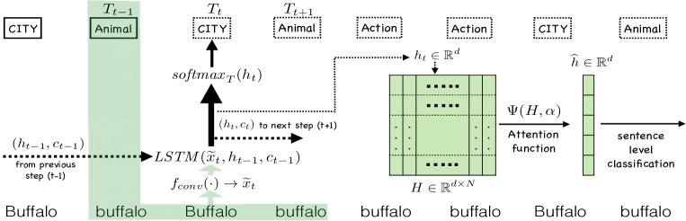
Figure 3: Jointly trained sequence labeling and sentence classification. The green mask means that convolution operate between one previous tag and two surrounding words (when window size is 3). $\Psi$ is the attention function in Eq. 5. Here the sentence length is $N$=8.

We use LSTM to model the representation of the sentence at each word step, which is powerful in modeling sentence semantics [7, 8]. Assume the length of the sentence is $N$. LSTM represents the meaning of the sentence at the $t$-th word by a pair of vectors $(h_{t},c_{t})\in(\mathbb{R}^{d},\mathbb{R}^{d})$, where $h_{t}$ is the output hidden representation of the word, $c_{t}$ is the memory of the network, and $d$ is the number of dimensions of the representation space:

$$\begin{bmatrix}i_{t}\\ f_{t}\\ o_{t}\\ \hat{c}_{t}\end{bmatrix}=\begin{bmatrix}\sigma\\ \sigma\\ \sigma\\ \text{tanh}\end{bmatrix}W_{\text{LSTM}}\cdot[x_{t},h_{t-1}]$$ (1)

$$c_{t}=f_{t}\odot c_{t-1}+i_{t}\odot\hat{c}_{t}$$ (2)

$$h_{t}=o_{t}\odot\text{tanh}(c_{t})$$ (3)

Here $x_{t}$ represents the $t$-th word, which is usually the word embedding vector, and vectors $i_{t},f_{t}$, and $o_{t}$ are gated activations that control flow of hidden information. The separation of the output representation $h_{t}$ from its internal memory $c_{t}$, in principle, makes the knowledge about the sentence prefix be remembered by the network for longer time to interfere with the current output at word $x_{t}$. These carefully designed activation gates alleviate the problem of vanishing gradient problem in vanilla recurrent neural network models.

In the task of sequence labeling, the label for each word is determined by hidden representation $h_{t}$. As described in Eq. 3, at time step $t$, we will get an output $h_{t}$ which represents all the current information. The probability distribution of the $t$-th word’s label is calculated by $\mathit{softmax}_{T}(W_{T}\cdot h_{t})$, where weight $W_{T}\in\mathbb{R}^{d\times{\lvert T\rvert}}$ maps $h_{t}$ to the space of the labels, and $\lvert T\rvert$ is the number of possible labels. For the sequence labeling problem, the loss $\ell_{\text{seq}}$ is calculates as the sum of the Negative Log-Likelihood (NLL) over this label distribution $\mathit{softmax}_{T}(h_{t})$ at each time step.

In the task of sentence classification, the entire sentence representation is obtained by aggregating all history outputs $h_{t}$ which are stored in $H\in\mathbb{R}^{d\times N}$, where $N$ is the length of sequence. Similar to CNNs, max pooling [9, 10, 11] operates over the history outputs $H$ to get the average activation $\hat{h}=\mathit{pooling}(H)$ summarizing the entire outputs. Then, this sentence representation is passed to a fully connected soft-max layer which outputs a distribution over sentence categories.

In above two different tasks, the hidden representation $h_{t}$ functions as a key component in different, separate ways. In many cases, when sequence-level labels and sentence categories are both available we should use both information within the same framework by joint training the two tasks.

3 Joint Sequence Classification & Labeling

3.1 Joint Training Model

Table 1: Examples of ATIS sentences and annotated slots and categories.

Sentence 1	I	want	to	go	from	Denver	to	Boston	today	Category
Slots	O	O	O	O	O	B-FromCity	O	B-ToCity	B-Date	Flight
Sentence 2	to	come	back	to	Los	Angeles	on	Friday	evening	Category
Slots	O	O	O	O	B-ReturnCity	I-ReturnCity	O	B-RETURN.DAY	B-RETURN.PERIODOFDAY	Return

We aim at developing a model which could learn the label sequence and sentence-level category simultaneously. To this end, we modify the standard LSTM structure to generate the word labels on the fly based on output $h_{t}$, and predict the sentence category with the sequence of $h_{t}$, $t=1,\dots,N$.

In LSTM, at time step $t$, only information of the current word $x_{t}$ is being fed into the network. This mechanism overlooks the problem that the meanings of the same word in different contexts might vary (cf. Fig. 2). In particular, words that follow $x_{t}$ are not represented at step $t$ in LSTM.

This observation motivates us to include more contextual information around the current word and previous tags as part of the input to LSTM. We employ convolutional neural network (CNN) to automatically mine the meaningful knowledge from both the context of word $x_{t}$ and previous tags $T_{t-1}$, and use this knowledge as the input for LSTM. We formally define the new input for LSTM as:

$$\vspace{-1mm}\widetilde{x}_{t}=f_{\text{conv}}(W_{\text{conv}}\cdot x_{t,k}+b_{\text{conv}})$$ (4)

where $f_{\text{conv}}$ is a non-linear activation function like rectified linear unit (ReLU) or sigmoid, and $x_{t,k}$ is a vector representing the context of word $x_{t}$ and previous tags $T_{t-k}...T_{t-1}$, e.g., the concatenation of the surrounding words and previous tags, $x_{t,k}=[x_{t-k},\dots,x_{t+k},\text{\hbox{\pagecolor{lightgray}$T_{t-k},\dots,T_{t-1}\!$}}]$ in Eq. 4, where the convolution window size is $2k+1$ and ${T_{t-1}}$ represents the embedding for tag $T_{t-1}$. $W_{\text{conv}}$ is the collection of filters applied on the context. During the convolution, each row of $W_{\text{conv}}$ is a filter that will be fired if it matches some useful pattern in the input context. The convolutional layer functions as a feature extraction tool to learn meaningful representation from both words and tags automatically. Note that the above contextual representation is different from bi-LSTM which only learns surrounding contextual of a given word. However, our model can learn both contextual and label information by convolution.

In our model, the joint training between sentence-level classification and sequential labeling is done in two directions: in forward pass, word label representation sequence is used for sentence level classification; during backward training, the sentence level prediction errors also fine-tune the label sequence.

Fig. 3 illustrates our proposed model with one classical NLP exemplary sentence which only contains the word “buffalo” as the running example. At each time step, we first use the convolutional layer as a feature extractor to get the nonlinear feature combinations from the embeddings of words and tags. In the case of window size equaling to 1, the convolution operates over the $t-1$, $t$ and $t+1$ words and the $t-1$ tag. The contextual representation $x_{t,1}=[x_{t-1},x_{t},x_{t+1},T_{t-1}]$ is then fed into the convolution layer to find feature representation $\widetilde{x}_{t}$ following Eq. 4. $\widetilde{x}_{t}$ is used as the input for the following LSTM to generate $h_{t}$ and $c_{t}$, based on history information $h_{t-1}$ and previous cell information $c_{t-1}$.

The example in Fig 3 is a grammatically correct sentence in English [12]. The word “buffalo” has three different meanings: Buffalo, NY (city), bison (animal), or bully (action). It is hard for standard LSTM to differentiate the different meanings of “buffalo” in different time step since the $x_{t}$ is the same all the time. However, in our case, instead of simply using word representation $x_{t}$ itself, we also consider the contextual information with their tags through convolution from $x_{t,k}$ (Eq. 4).

3.2 Sparse Attention

In the previous section, the sentence-level representation $\hat{h}$ is obtained by a simple average pooling on $H$. This process assumes every words contribute to the sentence equally, which is not the case in many scenarios. Fig. 2 shows a few examples of different words with different magnitudes of attention in different sentence categories. In order to incorporate these differences into consideration, we further propose a novel sparse attention constraint for sentence level classification. The sparse constraint assigns bigger weights for important words and lower the weights or even totally ignores the less meaningful words such like “the” or “a”. The attention-based sentence-level representation is formulated as follows:

$$\vspace{-2mm}\begin{split}\widehat{h}=\Psi(H,\alpha)=\sum_{h_{t}\in H}\psi(h_{t}\cdot\alpha)h_{t}\end{split}$$ (5)

where $\alpha\in\mathbb{R}^{d}$ is an attention measurement which decides the importances for different inputs based on their semantics $h_{i}$. This importance is calculated through a nonlinear function $\psi$ which can be sigmoid or ReLU and we use sigmoid in our case.

Sparse Autoencoders [13, 14] show that getting sparse representations in the hidden layers can further improve the performance. In our model, we apply similar sparse constraints by first calculating the average attention over the training samples in the same batch:

$$\vspace{-2mm}\hat{\rho}_{t}=\frac{1}{m}\sum_{i=1}^{m}\psi(h_{t}^{i}\cdot\alpha)\vspace{-1mm}$$ (6)

where $m$ is the size of training batch, and $h_{t}^{i}$ is the output of LSTM at step $t$ for example $i$. In order to keep the above attention within a fix budget, similar to Sparse Autoencoders [13], we have an extra penalty term as follows:

$$\mathit{KL}(\rho||\hat{\rho}_{t})=\rho\log\frac{\rho}{\hat{\rho}_{t}}+(1-\rho)\log\frac{1-\rho}{1-\hat{\rho}_{t}},$$

where $\rho$ is the desired sparsity of the attention. This penalty term uses KL divergence to measure the difference between two distributions. Then our new objective is defined as follows:

$$\ell_{\text{sparse}}(\cdot)=\ell_{\text{seq}}(\cdot)+\ell_{\text{sent}}(\cdot)+\beta\sum_{t=1}^{N}\mathit{KL}(\rho||\hat{\rho}_{t}),\vspace{-1mm}$$ (7)

where $N$ is the number of hidden units, $\ell_{\text{seq}}$ is the sequence labeling loss, and $\ell_{\text{sent}}$ is the sentence classification loss. $\beta$ controls the weight of the sparsity penalty term. Note that the term $\hat{\rho}_{t}$ is implicitly controlled by optimizing $\alpha$ and output $h_{t}$.

3.3 Label Sequence as Latent Variable

In practice, it is expensive to annotate the data with both sequential label and sequence category. In many cases, the sequence labels are missing since it requires significantly more efforts to annotate the labels word-by-word. However, even without this sequence labeling information, it is still helpful if we could utilize the possible hidden labels for each words.

In our proposed model, we could consider the sentence-level classification task as the major learning objective and treat the unknown sequence labels as latent information. The only adaptation we need to make is to replace the $T_{t}$ (tag embedding) with $h_{t}$ (output at time step $t$) in $x_{t,k}$. In this case, we exploit the latent meaning representation to further improve the feature extraction of the convolutional layer.

4 Experiments

Table 2: Main results: Our jointly trained models compared with various independent (marked ^†) and exisiting joint models. The “Slot” column shows the F1 score of sequence labeling, and “intent” shows the error rates for sentence classification.

	Model	Slot	Intent
Independent Model	CRF [4]	90.67†	7.91†
	CNN [5]	92.43†	6.65†
CRF Joint Model	TriCRF [4]	94.42 6.93
	CNN TriCRF [5]	95.42 5.91
Independent Model	Vanilla LSTM (baseline)	93.74†	7.21†
	+ joint	95.54 6.32
Jointly Trained Model	+ joint + CNN	97.35 5.96
(Secs. 3.1 & 3.2)	+ joint + CNN + attention	96.73 5.71
	+ joint + CNN + sparse att.	96.98 5.12
Independent Model	Vanilla LSTM (baseline)	-	7.21†
Seq. Label as Latent Var.	+ joint + CNN	-      6.43
(Sec. 3.3)	+ joint + CNN + attention	-      5.61
	+ joint + CNN + sparse att.	-      5.42

Model	Sent. Acc.
CNN non-static [10]	93.6
CNN multichannel [10]	92.2
Deep CNN [15]	93.0
Independent LSTM (baseline)	92.2
latent LSTM + CNN	92.6
latent LSTM + CNN + attention	93.4
latent LSTM + CNN + sparse att.	94.0

Figure 4: Sentence-level accuracy of our latent-variable model on TREC, compared with various neural network-based models.

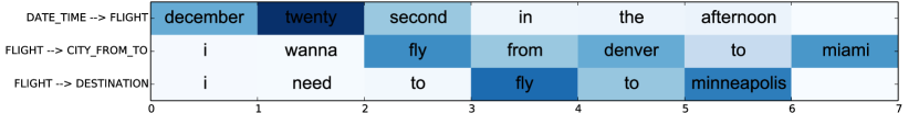
(a)

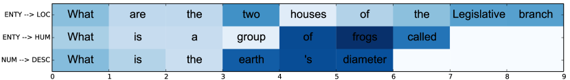
(b)

Figure 5: Examples that we outperform the model without sparse attention (LSTM+CNN). Higher weights are darker.

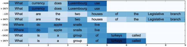
Figure 6: Comparison between softmax-based attention (upper) and sparse attention (lower) for for some examples. The sign ‘-’ means mis-classified label, and ‘+’ for the correct label. Darker blue represents higher weights.

We start by evaluating the performance on a conventional joint learning task (Sec. 4.1). Then we show the performance when we treat the label sequence as hidden information in Sec. 4.2. We also analyze some concrete examples to show the performance of the sparse attention constraint in our model (Sec. 4.3).

In the experiments, we set the convolution window sizes as 3, 5, and 7. There are 100 different filters for each window size. Word embeddings are randomly initialized in the ATIS experiments. In the TREC experiments, we use $300$ dimension pre-trained word embeddings. We use AdaDelta for optimization [16] with learning rate $0.001$ and minibatch 16. The weights in our framework are uniformly randomly initialized between $[-0.05,0.05]$. We use ReLu at the convolutional layer and also regularize the feature with dropout 0.5 [17].

We evaluate on ATIS[4] and TREC [18] datasets. We follow the TriCRF paper[4] in our evaluation on ATIS. There are $5,138$ dialogs with 21 types of intents and 110 types of slots annotated . This dataset is first used for joint learning model with both slot and intent labels in the joint learning experiments (Sec. 4.1). We later use it for evaluating the performance when the slot labels are not available (Sec. 4.2). The TREC dataset is a factoid question classification dataset, with $5,952$ sentences being classified into 6 categories. Since only the sentence-level categories are annotated, we treat the unknown tags as latent information in our experiments (Sec. 4.2).

4.1 Joint Training Experiments

We first perform the joint training experiments on the ATIS dataset. Tab. 1 shows two examples from the ATIS dataset. As mentioned in Sec. 3.2, only a few keywords in the two sentences in Tab. 1 are relevant to determining the category, i.e., locations (cities) and date for sentence I, and locations, date, and time for sentence II. Our model should be able to recognize these important keywords and predict the categories mostly based on them. Once the model knows the tags of the words in the sentence, it is straightforward to determine the categories of the sentence.

We show the performance of our model comparing with other individually trained or jointly trained models in Tab. 2. We observe that due to its strong generalization power, neural networks based models outperform discrete models with an impressive margin. Our jointly trained neural model achieves the best performance, with an F1 boost of $\sim$2 points in slot filling. After adding the sparse attention constraint, our model achieves the lowest error rate for the sentence classification on ATIS.

4.2 Label Sequence as Latent Variable

We further show the performance of our jointly trained model when the sequence label information is missing. Tab. 2 (bottom) shows the results on ATIS dataset. There is a small increase of error rate when sequence labels are unobserved, but our model still outperforms existing models. Similarly, Fig. 5 compares our latent-variable model with conventional (non-latent) neural models on TREC dataset (in sentence category accuracy). Our model outperforms others after adding sparse attention.

4.3 Sparsity Visualization

In Fig. 5, we compare the sparse attention model to the model without sparse constraints. We list a few examples that the sparse attention is better than the one without sparse attention constraint. The labels on the right side are mis-classified by the model without sparse attention constraint. The label on the left side of the arrow is the ground truth.

In Fig. 6, we also compare the difference between two attention mechanisms: softmax-based attetion and sparse attention. From the first sentence, we can tell that softmax-based attention puts more emphasis on “Luxembourg” while sparse attention prefers “currency” which leads to the correct prediction of entity instead of human. In some cases, like the third example in Fig. 6, softmax-based sometimes gets confused by distributing the probabilities flatly. Compared with the attention model between dual sentences, the phenomenon of flat distribution is more obvious in single sentence attention. Similar results can be found in the first figure in [20] as the word “run” is aligned to many unrelated words. It is possible that in single sentence attention, the softmax-based attention is easier to get confused since there is no obvious alignment or corresponding relationship between words for a given sentence or the words and their corresponding sentence category.

5 Related Works

One neural network based model is proposed in [19] for joint modeling the two tasks above with a parse-tree-based Recursive Neural Networks (RecNNs). However, as shown in their experiments, RecNNs fail to outperform most baselines. RecNNs-based jointly trained model is limited by two reasons: RecNNs’s performance highly depends on the quality of parse-trees which are treated as inputs together with sentences; another problem of RecNNs is shared with all other Recurrent Neural Networks (RNN) based models which is hard to train due to gradient vanishing and exploding [21]. When sentences get longer and parse-trees get deeper, RecNNs become harder to train.

Our sparse attention model is different from other attention models in the following aspects: Firstly, sparse attention is trained within one sentence. The goal is to find the most meaningful words which contribute to better sentence representation. This is different from dual sequences attention models [22, 23, 24]. Secondly, most attention models are softmax-based which gives a distribution over word or words. Softmax-based model has an exclusive property which allows cross influence between the source-side words. However, in sparse attention, this cross influence is not always necessary. The sum of attentions with sparse constraints does not have to be 1. Especially, our sparse attention is different from sparsemax attention [25]. Sparsemax tries to assign exactly zero probability to some of its output variables, but we try to control the sparsity of attention by adjusting $\rho$ and $\beta$. There are also neural-based efforts which only predict sequential labels, e.g., [26, 27].

6 Conclusions

We have presented a neural model that is jointly trained on the two tasks of sentence classification and sequence labeling, which benefits from the correlation between the two tasks. Our proposed models outperform both independent baselines and existing joint models, reaching the state-of-the-art in either sentence classification or sequence labeling.

7 Acknowledgment

This work is supported in part by NSF IIS-1656051, DARPA FA8750-13-2-0041 (DEFT), DARPA N66001-17-2-4030 (XAI), a Google Faculty Research Award, and an HP Gift.

References

- [1] B. E. Boser, I. M. Guyon, and V. N. Vapnik, “A training algorithm for optimal margin classifiers,” in Proceedings of the Fifth Annual Workshop on Computational Learning Theory, 1992.
- [2] J. D. Lafferty, A. McCallum, and F. C. N. Pereira, “Conditional random fields: Probabilistic models for segmenting and labeling sequence data,” in Proceedings of the Eighteenth International Conference on Machine Learning, 2001.
- [3] M. Collins, “Discriminative training methods for hidden markov models: Theory and experiments with perceptron algorithms,” in Proceedings of EMNLP, 2002.
- [4] M. Jeong and G. G. Lee, “Triangular-Chain Conditional Random Fields,” Audio, Speech, and Language Processing, IEEE Transactions on, vol. 16, 2008.
- [5] P. Xu and R. Sarikaya, “Convolutional neural network based triangular crf for joint intent detection and slot filling.” in ASRU. IEEE, 2013, pp. 78–83.
- [6] S. Hochreiter and J. Schmidhuber, “Long short-term memory,” Cambridge, MA, USA, 1997.
- [7] I. Sutskever, O. Vinyals, and Q. V. Le, “Sequence to sequence learning with neural networks,” in Advances in neural information processing systems, 2014, pp. 3104–3112.
- [8] J. Cheng, L. Dong, and M. Lapata, “Long short-term memory-networks for machine reading,” 2016.
- [9] R. Collobert, J. Weston, L. Bottou, M. Karlen, K. Kavukcuoglu, and P. Kuksa, “Natural language processing (almost) from scratch,” vol. 12, 2011, pp. 2493–2537.
- [10] Y. Kim, “Convolutional neural networks for sentence classification,” in Proceedings of the 2014 Conference on Empirical Methods in Natural Language Processing, 2014.
- [11] M. Ma, L. Huang, B. Xiang, and B. Zhou, “Dependency-based convolutional neural networks for sentence embedding,” in Proceedings of ACL 2015, 2015.
- [12] W. J. Rapaport, “A history of the sentence ”buffalo buffalo buffalo buffalo buffalo.”,” 2012. [Online]. Available: http://www.cse.buffalo.edu/~rapaport/buffalobuffalo.html
- [13] A. Ng, “Sparse autoencoder,” 2011. [Online]. Available: https://web.stanford.edu/class/cs294a/sparseAutoencoder.pdf
- [14] A. Makhzani and B. Frey, “K-sparse autoencoders,” in International Conference on Learning Representations, 2014.
- [15] N. Kalchbrenner, E. Grefenstette, and P. Blunsom, “A convolutional neural network for modelling sentences,” in ACL, 2014.
- [16] M. Zeiler, “Adadelta: An adaptive learning rate method,” Unpublished manuscript: http://arxiv.org/abs/1212.5701, 2012.
- [17] G. E. Hinton, N. Srivastava, A. Krizhevsky, I. Sutskever, and R. Salakhutdinov, “Improving neural networks by preventing co-adaptation of feature detectors,” Journal of Machine Learning Research, vol. 15, 2014.
- [18] X. Li and D. Roth, “Learning question classifiers,” in Proceedings of the 19th International Conference on Computational Linguistics - Volume 1, 2002.
- [19] D. Guo, G. Tur, W.-T. Yih, and G. Zweig, “Joint semantic utterance classification and slot filling with recursive neural networks,” in IEEE Workshop on Spoken Language Technology (SLT), 2014.
- [20] J. Cheng, L. Dong, and M. Lapata, “Long short-term memory-networks for machine reading,” arXiv preprint arXiv:1601.06733, 2016.
- [21] R. Pascanu, T. Mikolov, and Y. Bengio, “On the difficulty of training recurrent neural networks,” in Proceedings of the 30th International Conference on Machine Learning, 2013.
- [22] D. Bahdanau, K. Cho, and Y. Bengio, “Neural machine translation by jointly learning to align and translate,” vol. abs/1409.0473, 2014.
- [23] T. Rocktäschel, E. Grefenstette, K. M. Hermann, T. Kočiskỳ, and P. Blunsom, “Reasoning about entailment with neural attention,” in Proceedings of ICLR 2016, 2016.
- [24] S. Wang and J. Jiang, “Learning natural language inference with lstm,” in Proceedings of NAACL, 2016.
- [25] A. F. T. Martins and R. F. Astudillo, “From softmax to sparsemax: A sparse model of attention and multi-label classification,” in Proceedings of the 33nd International Conference on Machine Learning, ICML 2016, New York City, NY, USA, June 19-24, 2016, 2016, pp. 1614–1623.
- [26] G. Mesnil, Y. Dauphin, K. Yao, Y. Bengio, L. Deng, D. Hakkani-Tur, X. He, L. Heck, G. Tur, D. Yu, and G. Zweig, “Using recurrent neural networks for slot filling in spoken language understanding.” IEEE Institute of Electrical and Electronics Engineers, March 2015.
- [27] K. Yao, B. Peng, Y. Zhang, D. Yu, G. Zweig, and Y. Shi, “Spoken language understanding using long short-term memory neural networks.” IEEE Institute of Electrical and Electronics Engineers, December 2014. [Online]. Available: http://research.microsoft.com/apps/pubs/default.aspx?id=228844