Exceptional points in two simple textbook examples

Abstract

We propose to introduce the concept of exceptional points in intermediate courses on mathematics and classical mechanics by means of simple textbook examples. The first one is an ordinary second-order differential equation with constant coefficients. The second one is the well known damped harmonic oscillator. They enable one to connect the occurrence of linearly dependent exponential solutions with a defective matrix that cannot be diagonalized but can be transformed into a Jordan canonical form.

1 Introduction

Exceptional points[1, 2, 3, 4, 5] are being intensely studied because they appear to be suitable for the explanation of a wide variety of physical phenomena. Exceptional points (also called defective points[6] or non-Hermitian degeneracies[7]) appear, for example, in eigenvalue equations that depend on an adjustable parameter. As this parameter changes two eigenvalues approach each other and coalesce at an exceptional point. This coalescence is different from ordinary degeneracy because the two eigenvectors associated to the coalescing eigenvalues become linearly dependent at the exceptional point.

Numerical calculations predict the occurrence of exceptional points for the hydrogen atom in cross magnetic and electric fields[8] and it has been suggested that such points may be useful for estimating parameters of some atomic systems[9]. The predicted chirality of exceptional points has been verified in a variety of experiments[10, 11, 12, 13]. A detailed discussion of this experimental work is beyond the scope of this pedagogical communication. Many other articles about exceptional points are collected in the reference lists of those just mentioned.

The concept of exceptional point can be introduced by means of simple examples in intermediate courses on mathematics, quantum and classical mechanics. The purpose of this paper is the discussion of two examples that in our opinion are particularly appealing because they appear in courses of mathematics and classical physics at the undergraduate level. In section 2 we show the occurrence of exceptional points in ordinary differential equations with constant coefficients. Such problem is discussed in most textbooks on mathematics and differential equations[14]. In section 3 we discuss the well known problem of a damped harmonic oscillator when the friction force is proportional to the velocity of the oscillating particle[15]. This problem has already been chosen by Heiss[16] in his comment on experiments about encircling exceptional points[12, 13]. Here we enlarge upon this problem that may be of great pedagogical value. Finally, in section 4 we summarize the main results and draw conclusions.

2 Simple mathematical problem

In order to illustrate some of the features of an exceptional point we consider the second-order ordinary differential equation

$$\mathcal{L}(y)(x)=y^{\prime\prime}(x)+a_{1}y^{\prime}(x)+a_{0}y(x)=0,$$ (1)

with constant real coefficients $a_{i}$. One commonly obtains the solutions from the roots of the polynomial

$$e^{-\alpha x}\mathcal{L}(e^{\alpha x})(x)=\alpha^{2}+a_{1}\alpha+a_{0}=0,$$ (2)

that in this case are given by

$$\alpha_{1,2}=-\frac{a_{1}}{2}\pm\frac{1}{2}\sqrt{a_{1}^{2}-4a_{0}}.$$ (3)

The general solution is then[14]

$$y(x)=c_{1}e^{\alpha_{1}x}+c_{2}e^{\alpha_{2}x},$$ (4)

provided that $\alpha_{1}\neq\alpha_{2}$. The constants $c_{1}$ and $c_{2}$ are determined by the initial conditions; for example $y(0)=y_{0}$ and $y^{\prime}(0)=y_{1}$.

A problem arises when $a_{1}^{2}=4a_{0}$ because the two solutions are linearly dependent ($\alpha_{1}=\alpha_{2}=\alpha$). In this case the differential equation is given by

$$\mathcal{L}(y)=\left(\frac{d}{dx}-\alpha\right)^{2}y,$$ (5)

so that

$$\mathcal{L}\left(e^{\xi x}\right)=(\xi-\alpha)^{2}e^{\xi x}.$$ (6)

On taking into account that

$$\frac{d}{d\xi}\mathcal{L}\left(e^{\xi x}\right)=\mathcal{L}\left(xe^{\xi x}\right)=2(\xi-\alpha)e^{\xi x}+x(\xi-\alpha)^{2}e^{\xi x},$$ (7)

we appreciate that the two linearly independent solutions are $e^{\alpha x}$ and $xe^{\alpha x}$; that is to way

$$y(x)=c_{1}e^{\alpha x}+c_{2}xe^{\alpha x}.$$ (8)

Let us now approach the problem from another point of view. If we define $u=y^{\prime}$ then we can rewrite the second-order differential equation as a first-order one in matrix form

$$\frac{d}{dx}\left(\begin{array}[]{l}y\\ u\end{array}\right)=\mathbf{A}\left(\begin{array}[]{l}y\\ u\end{array}\right),\;\mathbf{A}=\left(\begin{array}[]{cc}0&1\\ -a_{0}&-a_{1}\end{array}\right).$$ (9)

The eigenvalues of the matrix $\mathbf{A}$ are exactly $\alpha_{1}$ and $\alpha_{2}$ and the corresponding unnormalized eigenvectors can be written as

$$\mathbf{v}_{1}=\left(\begin{array}[]{l}1\\ \alpha_{1}\end{array}\right),\;\mathbf{v}_{2}=\left(\begin{array}[]{l}1\\ \alpha_{2}\end{array}\right).$$ (10)

When $a_{0}<$ $a_{1}^{2}/4$ the two eigenvalues are real. As $a_{0}$ approaches $a_{1}^{2}/4$ they approach each other, coalesce at $a_{0}=a_{1}^{2}/4$ and become a pair of complex conjugate numbers for $a_{0}>$ $a_{1}^{2}/4$. Therefore, there is an exceptional point at $a_{0}=a_{1}^{2}/4$ where the matrix $\mathbf{A}$ becomes

$$\mathbf{A}=\left(\begin{array}[]{cc}0&1\\ -\alpha^{2}&2\alpha\end{array}\right),$$ (11)

because $a_{1}=-2\alpha$ and $a_{0}=\alpha^{2}$. Equation (10) clearly shows that $\mathbf{v}_{1}\rightarrow\mathbf{v}_{2}$ as $\alpha_{1}\rightarrow\alpha_{2}$ so that one eigenvector is lost at the exceptional point as outlined in the introduction.

It is therefore clear from the argument above that at the exceptional point the matrix $\mathbf{A}$ has only one eigenvalue and just one eigenvector

$$\mathbf{Av}_{1}=\alpha\mathbf{v}_{1},\;\mathbf{v}_{1}=\left(\begin{array}[]{l}1\\ \alpha\end{array}\right).$$ (12)

The matrix $\mathbf{A}$ is not normal ($AA^{T}\neq\mathbf{A}^{T}\mathbf{A}$, where $T$ stands for transpose) and at the exceptional point it becomes defective because it does not have a complete basis set of eigenvectors; consequently, it cannot be diagonalized.

Consider a second vector $\mathbf{u}_{2}$ that is a solution to the equation (Jordan chain[5])

$$\left(\mathbf{A}-\alpha\mathbf{I}\right)\mathbf{u}_{2}=\mathbf{v}_{1};$$ (13)

for example

$$\mathbf{u}_{2}=\left(\begin{array}[]{l}0\\ 1\end{array}\right).$$ (14)

The matrix

$$\mathbf{U}=\left(\mathbf{v}_{1}\mathbf{u}_{2}\right)=\left(\begin{array}[]{cc}1&0\\ \alpha&1\end{array}\right),$$ (15)

enables us to transform $\mathbf{A}$ into a Jordan canonical form

$$\mathbf{U}^{-1}\mathbf{AU}=\left(\begin{array}[]{cc}\alpha&1\\ 0&\alpha\end{array}\right).$$ (16)

It is not diagonal but has the eigenvalues in the diagonal. Defective matrices cannot be diagonalized but they can be transformed into Jordan matrices.

This simple mathematical problem shows the appearance of exceptional points in ordinary differential equations. At the exceptional point the exponential solutions become linearly dependent and we have to look for another type of solution. In addition to it, the matrix associated to the differential equation becomes defective and cannot be diagonalized but can instead be transformed into a Jordan matrix.

In closing this section we mention that the results shown above can be generalized to ordinary differential equations of order $n$ with constant coefficients

$$L(y)(x)=\sum_{j=0}^{n}a_{j}y^{(n)}(x)=0,$$ (17)

where $y^{(0)}(x)=y(x)$ and $y^{(j)}(x)=\frac{d}{dx}y^{(j-1)}$, $j=1,2,\ldots,n$. In order to obtain a matrix representation for this equation we simply consider the column vector with elements $y^{(j)}$, $j=0,2,\ldots,n-1$. We do not treat the general problem here because the greater number of independent parameters in the resulting $n\times n$ matrix makes the discussion of the exceptional points less appealing for pedagogical purposes.

3 Damped harmonic oscillator

In this section we discuss a simple physical model: the damped harmonic oscillator. A particle of mass $m$ moves in one dimension under the effect of a restoring force that follows the Hooke’s law: $f_{R}=-kx$, where $x$ is the displacement from equilibrium. We also assume that there is a damping force $f_{D}=-\gamma v$ that is proportional to the particle velocity $v=\dot{x}$, where the point indicates derivative with respect to time. This force is due to friction between the particle and the medium and the positive proportionality constant $\gamma$ is known as damping coefficient[15]. The Newton’s equation of motion for the particle is

$$m\ddot{x}=-kx-\gamma\dot{x}.$$ (18)

If we apply the results of section 2 with $a_{0}=k/m$ and $a_{1}=\gamma/m$ we have to describe the properties of the physical system in terms of two independent parameters. It is far more convenient to transform equation (18) into a dimensionless one with just one independent parameter.

In order to simplify the discussion of the model we define the dimensionless time $s=\omega_{0}t$, where $\omega_{0}=\sqrt{k/m}$ is the frequency of the oscillator when there is no damping. The resulting equation

$$y^{\prime\prime}(s)+y(s)+\lambda y^{\prime}(s)=0,$$ (19)

where $\lambda=\gamma/\left(m\omega_{0}\right)$ and $y(s)=x\left(s/\omega_{0}\right)$, is a particular case of (1) with $a_{0}=\lambda$ and $a_{1}=1$. The roots of the polynomial are

$$\alpha_{1,2}=-\frac{\lambda}{2}\pm\frac{1}{2}\sqrt{\lambda^{2}-4}.$$ (20)

When $\lambda<2$ ($\gamma<2m\omega_{0}$) the two roots are complex and the particle oscillates with frequency $\frac{1}{2}\sqrt{4-\lambda^{2}}<1$, or $\frac{\omega_{0}}{2}\sqrt{4-\lambda^{2}}<\omega_{0}$ (underdamped motion). The amplitude of the oscillation decreases exponentially as $\exp\left(-\frac{\lambda}{2}s\right)$ because of the loss of energy due to friction. If $\lambda>2$ the two roots are real and negative and the particle approaches the equilibrium position without any oscillation (overdamped motion). The particular case $\lambda=2$ is called critical damping and $y(s)=c_{1}e^{-s}+c_{2}se^{-s}$ as discussed in section 2. We appreciate that there is no oscillation as in the preceding case. The behaviour of this idealized physical system is discussed in detail in any introductory textbook on classical mechanics[15]; here we are mainly interested in the appearance of an exceptional point.

It is obvious, as discussed in section 2, that there is an exceptional point at $\lambda=2$. If we write the dimensionless equation of motion as

$$\frac{d}{ds}\left(\begin{array}[]{l}y\\ u\end{array}\right)=\mathbf{A}\left(\begin{array}[]{l}y\\ u\end{array}\right),\;\mathbf{A}=\left(\begin{array}[]{cc}0&1\\ -1&-\lambda\end{array}\right),$$ (21)

then the resulting matrix $\mathbf{A}$ cannot be diagonalized when $\lambda=2$. Following the procedure outlined in section 2 we can transform $\mathbf{A}$ into a Jordan matrix

$$\mathbf{U}^{-1}\mathbf{AU=}\left(\begin{array}[]{cc}-1&1\\ 0&-1\end{array}\right),\;\mathbf{U}=\left(\begin{array}[]{cc}1&0\\ -1&1\end{array}\right)$$ (22)

Figure 1 shows the real and imaginary parts of the roots $\alpha_{1}$ and $\alpha_{2}$ for $0\leq\lambda\leq 3$. They exhibit the well known branching pattern typical of exceptional points[4]. Note that these figures apply to any combination of values of $m$, $k$ and $\gamma$ and that the use of a dimensionless equation enables us to describe the main properties of the model in terms of only one independent parameter.

4 Conclusions

We think that the two examples discussed here are most suitable for the introduction of the concept of exceptional point in intermediate courses on mathematics and classical mechanics. The second-order ordinary differential equation with constant coefficients is already discussed in almost any textbook on mathematics or differential equations[14]. It shows the connection between the occurrence of linearly-dependent exponential solutions and the disappearance of one of the eigenvectors of the matrix associated to the differential equation. The second example is one of the simplest mechanical problems that exhibits friction and is also studied in elementary courses on classical physics[15]. In this case the exceptional point appears at the phase transition between underdamped and overdamped motion (critical damping). It is worth noting that the use of a dimensionless dynamical equation facilitates the analysis of the problem and the plotting the eigenfrequencies for arbitrary values of the model parameters: $m$, $k$ and $\gamma$. Instead of three parameters we need to consider the variation of only one $\lambda=\gamma/\sqrt{mk}$ that combines them in a suitable way.

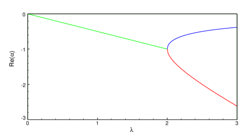
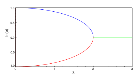
Figure 1: Real and imaginary parts of $\alpha_{1}$ and $\alpha_{2}$ for the damped harmonic oscillator

References

- [1] W. D. Heiss and A. L. Sannino, “Avoided level crossing and exceptional points”, J. Phys. A 23, 1167-1178 (1990).
- [2] W. D. Heiss, “Repulsion of resonance states and exceptional points”, Phys. Rev. E 61, 929-932 (2000).
- [3] W. D. Heiss and H. L. Harney, “The chirality of exceptional points”, Eur. Phys. J. D 17, 149-151 (2001).
- [4] W. D. Heiss, “Exceptional points - their universal occurrence and their physical significance”, Czech. J. Phys. 54, 1091-1099 (2004).
- [5] U. Günther, I. Rotter, and B. F. Samsonov, “Projective Hilbert space structures at exceptional points”, J. Phys. A 40, 8815-8833 (2007).
- [6] N. Moiseyev and S. Friedland, “Association of resonance states with the incomplete spectrum of finite complex-scaled Hamiltonian matrices”, Phys. Rev. A 22, 618-624 (1980).
- [7] M. V. Berry and D. H. J. O’Dell, “Diffraction by volume gratings with imaginary potentials”, J. Phys. A 31, 2093-2101 (1998).
- [8] H. Cartarius, J. Main, and G. Wunner, “Exceptional Points in Atomic Spectra”, Phys. Rev. Lett. 99, 173003 (2007).
- [9] M. Am-Shallem, R. Ronnie Kosloff, and N. Moiseyev, “Parameter estimation in atomic spectroscopy using exceptional points”, Phys. Rev. A 93, 032116 (2016).
- [10] C. Dembowski, H.-D. Gräf, H. L. Harney, A. Heine, W. D. Heiss, H. Rehfeld, and A. Richter, “Experimental Observation of the Topological Structure of Exceptional Points”, Phys. Rev. Lett. 86, 787-790 (2001).
- [11] C. Dembowski, B. Dietz, H.-D. Gräf, H. L. Harney, A. Heine, W. D. Heiss, and A. Richter, “Observation of a Chiral State in a Microwave Cavity”, Phys. Rev. Lett. 90, 013001 (2003).
- [12] J. Doppler, A. A. Mailybaev, J. Böhm, U. Kuhl, A. Girschik, F. Libisch, T. J. Milburn, P. Rabl, N. Moiseyev, and S. Rotter, “Dynamically encircling an exceptional point for asymmetric mode switching”, Nature 537, 76-79 (2016).
- [13] H. Xu, D. Mason, L. Jiang, and J. G. E. Harris, “Topological energy transfer in an optomechanical system with exceptional points”, Nature 537, 80-83 (2016).
- [14] T. Apostol, Calculus, Second ed. (John Wiley & Sons, New York, 1967).
- [15] M. R. Spiegel, Theoretical Mechanics, (Shaum, New York, 1967).
- [16] D. Heiss, “Circling exceptional points”, Nature Phys. 12, 823-824 (2016).