A Gaussian mixture model representation of endmember variability in hyperspectral unmixing

Abstract

Hyperspectral unmixing while considering endmember variability is usually performed by the normal compositional model (NCM), where the endmembers for each pixel are assumed to be sampled from unimodal Gaussian distributions. However, in real applications, the distribution of a material is often not Gaussian. In this paper, we use Gaussian mixture models (GMM) to represent endmember variability. We show, given the GMM starting premise, that the distribution of the mixed pixel (under the linear mixing model) is also a GMM (and this is shown from two perspectives). The first perspective originates from the random variable transformation and gives a conditional density function of the pixels given the abundances and GMM parameters. With proper smoothness and sparsity prior constraints on the abundances, the conditional density function leads to a standard maximum a posteriori (MAP) problem which can be solved using generalized expectation maximization. The second perspective originates from marginalizing over the endmembers in the GMM, which provides us with a foundation to solve for the endmembers at each pixel. Hence, compared to the other distribution based methods, our model can not only estimate the abundances and distribution parameters, but also the distinct endmember set for each pixel. We tested the proposed GMM on several synthetic and real datasets, and showed its potential by comparing it to current popular methods.

I Introduction

The formation of hyperspectral images can be simplified by the linear mixing model (LMM), which assumes that the physical region corresponding to a pixel contains several pure materials, so that each material contributes a fraction of its spectra based on area to the final spectra of the pixel. Hence, the observed spectra $\mathbf{y}_{n}\in\mathbb{R}^{B}$, $n=1,\dots,N$ ($B$ is the number of wavelengths and $N$ is the number of pixels) is a (non-negative) linear combination of the pure material (called endmember) spectra $\mathbf{m}_{j}\in\mathbb{R}^{B}$, $j=1,\dots,M$ ($M$ is the number of endmembers), i.e.

$$\mathbf{y}_{n}=\sum_{j=1}^{M}\mathbf{m}_{j}\alpha_{nj}+\mathbf{n}_{n},\,\text{s.t.}\,\alpha_{nj}\geq 0,\,\sum_{j=1}^{M}\alpha_{nj}=1,$$ (1)

where $\alpha_{nj}$ is the proportion (called abundance) for the $j$th endmember at the $n$th pixel (with the positivity and sum-to-one constraint) and $\mathbf{n}_{n}\in\mathbb{R}^{B}$ is additive noise. Here, the endmember set $\left\{\mathbf{m}_{j}:\,j=1,\dots,M\right\}$ is fixed for all the pixels. This model simplifies the unmixing problem to a matrix factorization one, leading to efficient computation and simple algorithms such as iterative constrained endmembers (ICE), vertex component analysis (VCA), piecewise convex multiple-model endmember detection (PCOMMEND) [1, 2, 3] etc., which receive comprehensive reviews in [4, 5].

However, in practice the LMM may not be valid in many real scenarios. Even for a pure pixel that only contains one material, its spectra may not be consistent over the whole image. This is due to several factors such as atmospheric conditions, topography and intrinsic variability. For example, in vegetation, multiple scattering and biotic variation (e.g. differences in biochemistry and water content) cause different reflectances among the same species. For urban scenes, the incidence and emergence angles could be different for the same roof, causing different reflectances. For minerals, the spectroscopy model developed by Hapke also considers the porosity and roughness of the material as variable [6].

In the first and third example above, Eq. (1) can be generalized to a more abstract form $\mathbf{y}_{n}=F\left(\left\{\mathbf{m}_{j},\alpha_{nj}:\,j=1,\dots M\right\}\right)$, which leads to nonlinear mixing models. For example, in [7] the authors used bilinear models to handle the vegetation case, which was also investigated using several different nonlinear functions [8]. In [9], the Hapke model was used to model intimate interaction among minerals. There are also works that use kernels for flexible nonlinear mixing [10, 11]. A panoply of nonlinear models can be found in the review article [12]. We note that in these models, a fixed endmember set is still assumed while using a more complicated unmixing model.

While nonlinear models abound lately, it is still difficult to account for all the scenarios. On the contrary, the LMM still has physical significance with the intuitive area assumption. To model real scenarios more accurately, researchers have taken another route by generalizing Eq. (1) to

$$\mathbf{y}_{n}=\sum_{j=1}^{M}\mathbf{m}_{nj}\alpha_{nj}+\mathbf{n}_{n},$$ (2)

where $\left\{\mathbf{m}_{nj}\in\mathbb{R}^{B}:\,j=1,\dots,M\right\},\,n=1,\dots,N$ could be different for each $n$, i.e. the endmember spectra for each pixel could be different. This is called endmember variability, and has also received a lot of attention in the community [13, 14]. Note that given $\left\{\mathbf{y}_{n}\right\}$, inferring $\left\{\mathbf{m}_{nj},\alpha_{nj}\right\}$ is a much more difficult problem than inferring $\left\{\mathbf{m}_{j},\alpha_{nj}\right\}$ in Eq. (1). Hence, in many papers $\left\{\mathbf{m}_{nj}\right\}$ are assumed to be from a spectral library, which is usually called supervised unmixing [15, 16, 17]. On the other hand, if the endmember spectra are to be extracted from the image, we call them unsupervised unmixing models [18, 19, 20]. Obviously, unsupervised unmixing is more challenging than its supervised counterpart and hence more assumptions are used in this case, such as the spatial smoothness of abundances and endmember variability [21, 22, 23], small mutual distance between the endmembers [22], small magnitude or spectral smoothness of the endmember variability [22, 23].

We can also categorize the papers on endmember variability by how this variability is modeled. In the review paper [14], it can be modeled as a endmember set [20, 17] or as a distribution [24, 25, 26]. One of the widely used set based methods is multiple endmember spectral mixture analysis (MESMA) [17], which tries every endmember combination and selects the one with the smallest error. There are many variations to the original MESMA. For example, the multiple-endmember linear spectral unmixing model (MELSUM) solves the linear equations directly using the pseudo-inverse and discards the solutions with negative abundances [27]; automatic Monte Carlo unmixing (AutoMCU) picks random combinations for unmixing and averages the resulting abundances as the final results [28, 29]. Besides MESMA variants, there are also many other set based methods. For example, endmember bundles form bundles from automated extracted endmembers, take minimum and maximum abundances from bundle based unmixing, and average them as final abundances [20]; sparse unmixing imposes a sparsity constraint on the abundances based on endmembers composed of all spectra from the spectral library [30]. A comprehensive review can be found in [13, 14]. One disadvantage of set based methods is that their complexity increases exponentially with increasing library size hence in practice a laborious library reduction approach may be required [31].

The distribution based approaches assume that the endmembers for each pixel are sampled from probability distributions [e.g. Gaussian, a.k.a. normal compositional model (NCM)], and hence embrace large libraries while being numerically tractable [15, 32]. Here, we give an overview of NCM because of its simplicity and popularity [19, 18, 16]. Suppose the jth endmember at the nth pixel follows a Gaussian distribution $p\left(\mathbf{m}_{nj}\right)=\mathcal{N}\left(\mathbf{m}_{nj}|\boldsymbol{\mu}_{j},\boldsymbol{\Sigma}_{j}\right)$ where $\boldsymbol{\mu}_{j}\in\mathbb{R}^{B}$ and $\boldsymbol{\Sigma}_{j}\in\mathbb{R}^{B\times B}$, and the additive noise also follows a Gaussian distribution $p\left(\mathbf{n}_{n}\right)=\mathcal{N}\left(\mathbf{n}_{n}|\mathbf{0},\mathbf{D}\right)$ where $\mathbf{D}$ is the noise covariance matrix. The random variable transformation (r.v.t.) (2) suggests that the probability density function of $\mathbf{y}_{n}$ can be derived as

$$p\left(\mathbf{y}_{n}|\boldsymbol{\alpha}_{n},\boldsymbol{\Theta},\mathbf{D}\right)=\mathcal{N}\left(\mathbf{y}_{n}|\sum_{j=1}^{M}\alpha_{nj}\boldsymbol{\mu}_{j},\sum_{j=1}^{M}\alpha_{nj}^{2}\boldsymbol{\Sigma}_{j}+\mathbf{D}\right),$$ (3)

where $\boldsymbol{\alpha}_{n}\vcentcolon=\left[\alpha_{n1},\dots,\alpha_{nM}\right]^{T}$, $\boldsymbol{\Theta}\vcentcolon=\left\{\boldsymbol{\mu}_{j},\boldsymbol{\Sigma}_{j}:\,j=1,\dots,M\right\}$. The conditional density function in (3) is usually embedded in a Bayesian framework such that we can incorporate priors and also estimate hyperparameters. Then, NCM uses different optimization approaches, e.g. expectation maximization [32], sampling methods [19, 25, 18], particle swarm optimization [24], to determine the parameters $\left\{\boldsymbol{\mu}_{j},\boldsymbol{\Sigma}_{j}\right\}$ and $\left\{\alpha_{nj}\right\}$.

There are few papers that use other distributions. In [15], Xiaoxiao Du et al. note that the Gaussian distribution may allow negative values which are not realistic. In addition, the real distribution may be skewed. Hence, they introduce a Beta compositional model (BCM) to model the variability. The problem is that the true distribution may not be well approximated by any unimodal distribution. Consider the Pavia University dataset shown in Fig. 1, where the multidimensional pixels are projected to one dimension to afford better visualization. Among the manually identified materials, we can see that although the histogram of meadows may look like a Gaussian distribution, that of painted metal sheets has multiple peaks and cannot be approximated by either a Gaussian or Beta distribution. This is due to different angles of these sheets on the roof. Since each piece of metal sheet is tilted, it forms a cluster of reflectances which contributes to a peak in the histogram. This example shows that we should use a more flexible distribution to represent the endmember variability.

Figure 1: (a) Original Pavia University image and selected ROI with its ground truth image. (b) Mean spectra of the identified 5 endmembers and histograms of meadows and painted metal sheets (shadow is termed as endmember to conform with the LMM though the area under shadow can be any material). PCA is used to project the multidimensional pixels to single values which are counted in the histograms. Although the histogram of meadows may appear to be a Gaussian distribution, that of painted metal sheets is obviously neither a unimodal Gaussian or Beta distribution.

In this paper, we use a mixture of Gaussians to approximate any distribution that an endmember may exhibit, and solve the LMM by considering endmember variability. In a nutshell, the Gaussian mixture model (GMM) models $p\left(\mathbf{m}_{nj}\right)$ by a mixture of Gaussians, say $p\left(\mathbf{m}_{nj}\right)=\sum_{k}\pi_{jk}\mathcal{N}\left(\mathbf{m}_{nj}|\boldsymbol{\mu}_{jk},\boldsymbol{\Sigma}_{jk}\right)$, and then obtains the distribution of $\mathbf{y}_{n}$ by the r.v.t. (2), which turns out to be another mixture of Gaussians and can be used for inference of the unknown parameters. Here, we briefly explain how GMM works intuitively by comparing it to the NCM with the details given later. The maximum likelihood estimate (MLE) of NCM (using (3)) aims to find $\left\{\boldsymbol{\mu}_{j}\right\}$ such that its linear combination matches $\mathbf{y}_{n}$. Contrary to NCM, GMM aims to find $\left\{\boldsymbol{\mu}_{jk}\right\}$ such that all of its linear combinations match $\mathbf{y}_{n}$. Suppose we have $\boldsymbol{\mu}_{11}$, $\boldsymbol{\mu}_{21}$, $\boldsymbol{\mu}_{22}$, $\boldsymbol{\mu}_{31}$, $\boldsymbol{\mu}_{32}$, $\boldsymbol{\mu}_{33}$: then there are 6 combinations as explained in Fig. 2, but with emphasis weighted by $\left\{\pi_{jk}\right\}$ which determines the prior probability of each linear combination.

Figure 2: Comparison of the mechanisms among LMM, NCM and GMM. We have 3 endmembers represented by the darken gray areas. LMM tries to find a set of endmembers that fit the pixel data. NCM tries to find a set of Gaussian centers that fit the pixel data, with error weighted by the covariance matrices. GMM tries to find Gaussian centers such that all their linear combinations fit the pixel data, with each weighted by the prior $\pi_{\mathbf{k}}$. We may use 6 endmembers with NCM, but then the prior information is lost.

Based on the GMM formulation, we propose a supervised version and an unsupervised version for unmixing. The supervised version takes a library as input and estimates the abundances. The unsupervised version assumes that there are regions of pure pixels, hence segments the image first to get pure pixels and then performs unmixing. Another advantage over the other distribution based methods is that we can also estimate the endmembers for each pixel, which is not achievable by NCM or BCM. Note that estimating endmembers for each pixel is generally common in non-distribution methods, both from the signal processing community [22, 21, 23] or the remote sensing community [17, 27]. But it is often achieved in the context of least-squares based unmixing [33, 34, 35], unlike what we propose here using distribution based unmixing.

Notation: As usual, $\mathcal{N}\left(\mathbf{x}|\boldsymbol{\mu},\boldsymbol{\Sigma}\right)$ denotes the multivariate Gaussian density function with center $\boldsymbol{\mu}$ and covariance matrix $\boldsymbol{\Sigma}$. Let $\mathbf{A}\in\mathbb{R}^{m\times n}$ be a matrix with $m$ rows and $n$ columns. The Hadamard product of two matrices (elementwise multiplication) is denoted by $\circ$ while the Kronecker product is denoted by $\otimes$. $\left(\mathbf{A}\right)_{jk}$ denotes the element at the jth row and kth column of matrix $\mathbf{A}$. $\left(\mathbf{A}\right)_{j}$ denotes the jth row of $\mathbf{A}$ transposed (treating $\mathbf{A}$ as a vector), i.e. for $\mathbf{A}=\left[\mathbf{a}_{1},\dots\mathbf{a}_{n}\right]^{T}$, $\left(\mathbf{A}\right)_{j}=\mathbf{a}_{j}$. $\text{vec}\left(\mathbf{A}\right)$ denotes the vectorization of $\mathbf{A}$, i.e. concatenating the columns of $\mathbf{A}$. $\delta_{jk}=1$ when $j=k$ and 0 otherwise. $\mathbb{E}_{\mathbf{x}}\left(f\left(\mathbf{x}\right)\right)$ is the expected value of $f\left(\mathbf{x}\right)$ given random variable $\mathbf{x}$. We use $i=\sqrt{-1}$ instead of as an index throughout the paper.

II Mathematical Preliminaries

II-A Linear combination of GMM random variables

To use the Gaussian mixture model to model endmember variability, we start by assuming that $\mathbf{m}_{nj}$ follows a Gaussian mixture model (GMM) and the noise also follows a Gaussian distribution. The distribution of $\mathbf{y}_{n}$ is obtained using the following theorem.

Theorem 1.

If the random variable $\mathbf{m}_{nj}$ has a density function

$$p\left(\mathbf{m}_{nj}|\boldsymbol{\Theta}\right)\vcentcolon=f_{\mathbf{m}_{j}}\left(\mathbf{m}_{nj}\right)=\sum_{k=1}^{K_{j}}\pi_{jk}\mathcal{N}\left(\mathbf{m}_{nj}|\boldsymbol{\mu}_{jk},\boldsymbol{\Sigma}_{jk}\right),$$ (4)

s.t. $\pi_{jk}\geq 0,\,\sum_{k=1}^{K_{j}}\pi_{jk}=1$, with $K_{j}$ being the number of components, $\pi_{jk}$ ($\boldsymbol{\mu}_{jk}\in\mathbb{R}^{B}$ or $\boldsymbol{\Sigma}_{jk}\in\mathbb{R}^{B\times B}$) being the weight (mean or covariance matrix) of its kth Gaussian component, $\boldsymbol{\Theta}\vcentcolon=\left\{\pi_{jk},\boldsymbol{\mu}_{jk},\boldsymbol{\Sigma}_{jk}:\,j=1,\dots,M,k=1,\dots,K_{j}\right\}$, $\left\{\mathbf{m}_{nj}:\,j=1,\dots,M\right\}$ are independent, and the random variable $\mathbf{n}_{n}$ has a density function $p\left(\mathbf{n}_{n}\right):=\mathcal{N}\left(\mathbf{n}_{n}|\mathbf{0},\mathbf{D}\right)$, then the density function of $\mathbf{y}_{n}$ given by the r.v.t. $\mathbf{y}_{n}=\sum_{j=1}^{M}\mathbf{m}_{nj}\alpha_{nj}+\mathbf{n}_{n}$ is another GMM

$$p\left(\mathbf{y}_{n}|\boldsymbol{\alpha}_{n},\boldsymbol{\Theta},\mathbf{D}\right)=\sum_{\mathbf{k}\in\mathcal{K}}\pi_{\mathbf{k}}\mathcal{N}\left(\mathbf{y}_{n}|\boldsymbol{\mu}_{n\mathbf{k}},\boldsymbol{\Sigma}_{n\mathbf{k}}\right),$$ (5)

where $\mathcal{K}\vcentcolon=\left\{1,\dots,K_{1}\right\}\times\left\{1,\dots,K_{2}\right\}\times\cdots\times\left\{1,\dots,K_{M}\right\}$ is the Cartesian product of the $M$ index sets, $\mathbf{k}\vcentcolon=\left(k_{1},\dots k_{M}\right)\in\mathcal{K}$, $\pi_{\mathbf{k}}\in\mathbb{R}$, $\boldsymbol{\mu}_{n\mathbf{k}}\in\mathbb{R}^{B}$, $\boldsymbol{\Sigma}_{n\mathbf{k}}\in\mathbb{R}^{B\times B}$ are defined by

$$\pi_{\mathbf{k}}:=\prod_{j=1}^{M}\pi_{jk_{j}},\,\boldsymbol{\mu}_{n\mathbf{k}}\vcentcolon=\sum_{j=1}^{M}\alpha_{nj}\boldsymbol{\mu}_{jk_{j}},\,\boldsymbol{\Sigma}_{n\mathbf{k}}\vcentcolon=\sum_{j=1}^{M}\alpha_{nj}^{2}\boldsymbol{\Sigma}_{jk_{j}}+\mathbf{D}.$$ (6)

The proof is detailed using a characteristic function (c.f.) approach.

We first consider the distribution of the intermediate variable $\mathbf{z}_{n}=\sum_{j=1}^{M}\mathbf{m}_{nj}\alpha_{nj}$. The c.f. of $f_{\mathbf{m}_{j}}$ in (4), $\phi_{\mathbf{m}_{j}}\left(\mathbf{t}\right):\,\mathbb{R}^{B}\rightarrow\mathbb{C}$, is given by

$$\phi_{\mathbf{m}_{j}}\left(\mathbf{t}\right) =\mathbb{E}_{\mathbf{m}_{j}}\left(e^{i\mathbf{t}^{T}\mathbf{x}}\right)=\int_{\mathbb{R}^{B}}e^{i\mathbf{t}^{T}\mathbf{x}}f_{\mathbf{m}_{j}}\left(\mathbf{x}\right)d\mathbf{x}$$

$$=\sum_{k=1}^{K_{j}}\pi_{jk}\int_{\mathbb{R}^{B}}e^{i\mathbf{t}^{T}\mathbf{x}}\mathcal{N}\left(\mathbf{x}|\boldsymbol{\mu}_{jk},\boldsymbol{\Sigma}_{jk}\right)d\mathbf{x}$$

$$=\sum_{k=1}^{K_{j}}\pi_{jk}\phi_{jk}\left(\mathbf{t}\right),$$ (7)

where $\phi_{jk}\left(\mathbf{t}\right)$ denotes the c.f. of the Gaussian distribution $\mathcal{N}\left(\mathbf{x}|\boldsymbol{\mu}_{jk},\boldsymbol{\Sigma}_{jk}\right)$ as

$$\phi_{jk}\left(\mathbf{t}\right)\vcentcolon=\exp\left(i\mathbf{t}^{T}\boldsymbol{\mu}_{jk}-\frac{1}{2}\mathbf{t}^{T}\boldsymbol{\Sigma}_{jk}\mathbf{t}\right).$$ (8)

Assuming $\mathbf{m}_{n1},\dots,\mathbf{m}_{nM}$ are independent, we can obtain the c.f. of the linear combination of these $\mathbf{m}_{nj}$ by multiplying (7) as

$$\phi_{\mathbf{z}_{n}}\left(\mathbf{t}\right)=\phi_{\mathbf{m}_{n1}\alpha_{n1}+\cdots+\mathbf{m}_{nM}\alpha_{nM}}\left(\mathbf{t}\right)=\prod_{j=1}^{M}\phi_{\mathbf{m}_{j}}\left(\alpha_{nj}\mathbf{t}\right)$$

$$= \sum_{k_{1}=1}^{K_{1}}\cdots\sum_{k_{M}=1}^{K_{M}}\pi_{1k_{1}}\cdots\pi_{Mk_{M}}\phi_{1k_{1}}\left(\alpha_{n1}\mathbf{t}\right)\cdots\phi_{Mk_{M}}\left(\alpha_{nM}\mathbf{t}\right).$$

Let $\mathcal{K}$, $\mathbf{k}$, $\pi_{\mathbf{k}}$ be defined as in Theorem 1. We can write the above multiple summations in an elegant way:

$$\phi_{\mathbf{z}_{n}}\left(\mathbf{t}\right)=\sum_{\mathbf{k}\in\mathcal{K}}\pi_{\mathbf{k}}\phi_{n\mathbf{k}}\left(\mathbf{t}\right),$$ (9)

where $\pi_{\mathbf{k}}\geq 0$, $\sum_{\mathbf{k}\in\mathcal{K}}\pi_{\mathbf{k}}=1$ and

$$\phi_{n\mathbf{k}}\left(\mathbf{t}\right)\vcentcolon=\phi_{1k_{1}}\left(\alpha_{n1}\mathbf{t}\right)\cdots\phi_{Mk_{M}}\left(\alpha_{nM}\mathbf{t}\right)$$

$$= \exp\left\{i\mathbf{t}^{T}\left(\sum_{j=1}^{M}\alpha_{nj}\boldsymbol{\mu}_{jk_{j}}\right)-\frac{1}{2}\mathbf{t}^{T}\left(\sum_{j=1}^{M}\alpha_{nj}^{2}\boldsymbol{\Sigma}_{jk_{j}}\right)\mathbf{t}\right\},$$

where (8) is used. Since $\phi_{n\mathbf{k}}\left(\mathbf{t}\right)$ also has a form of c.f. of a Gaussian distribution, the corresponding distribution turns out to be $\mathcal{N}\left(\mathbf{x}|\sum_{j}\alpha_{nj}\boldsymbol{\mu}_{jk_{j}},\sum_{j}\alpha_{nj}^{2}\boldsymbol{\Sigma}_{jk_{j}}\right)$. Hence, the distribution of $\mathbf{z}_{n}$ can be obtained by the Fourier transform of (9)

$$f_{\mathbf{z}_{n}}\left(\mathbf{z}_{n}\right) =\frac{1}{\left(2\pi\right)^{B}}\int_{\mathbb{R}^{B}}e^{-i\mathbf{t}^{T}\mathbf{z}_{n}}\phi_{\mathbf{z}_{n}}\left(\mathbf{t}\right)d\mathbf{t}$$

$$=\frac{1}{\left(2\pi\right)^{B}}\int_{\mathbb{R}^{B}}e^{-i\mathbf{t}^{T}\mathbf{z}_{n}}\sum_{\mathbf{k}\in\mathcal{K}}\pi_{\mathbf{k}}\phi_{n\mathbf{k}}\left(\mathbf{t}\right)d\mathbf{t}$$

$$=\sum_{\mathbf{k}\in\mathcal{K}}\pi_{\mathbf{k}}\mathcal{N}\left(\mathbf{z}_{n}|\sum_{j=1}^{M}\alpha_{nj}\boldsymbol{\mu}_{jk_{j}},\sum_{j=1}^{M}\alpha_{nj}^{2}\boldsymbol{\Sigma}_{jk_{j}}\right),$$ (10)

which is still a mixture of Gaussians.

After finding the distribution of the linear combination, we can add the noise term to find the distribution of $\mathbf{y}_{n}$. Suppose the noise also follows a Gaussian distribution, $p\left(\mathbf{n}_{n}\right)\vcentcolon=f_{\mathbf{n}_{n}}\left(\mathbf{n}_{n}\right)=\mathcal{N}\left(\mathbf{n}_{n}|\mathbf{0},\mathbf{D}\right),$ where $\mathbf{D}$ is the noise covariance matrix. We assume that the noise at different wavelengths is independent ($\sigma_{k}^{2}$ being the noise variance of the $k$th band), i.e. $\mathbf{D}=\text{diag}\left(\sigma_{1}^{2},\sigma_{2}^{2},\dots,\sigma_{B}^{2}\right)\in\mathbb{R}^{B\times B}$ (if it is not independent, the noise can actually be easily whitened to be independent as in [36]). Its c.f. has the following form

$$\phi_{\mathbf{n}_{n}}\left(\mathbf{t}\right)=\exp\left(-\frac{1}{2}\mathbf{t}^{T}\mathbf{D}\mathbf{t}\right)$$ (11)

by (8). Then the c.f. of $\mathbf{y}_{n}$ can be obtained by multiplying (9) and (11) (as $\mathbf{z}_{n}$ and $\mathbf{n}_{n}$ are independent)

$$\phi_{\mathbf{y}_{n}}\left(\mathbf{t}\right) =\phi_{\mathbf{z}_{n}}\left(\mathbf{t}\right)\phi_{\mathbf{n}_{n}}\left(\mathbf{t}\right)=\sum_{\mathbf{k}\in\mathcal{K}}\pi_{\mathbf{k}}\phi_{\mathbf{n}_{n}}\left(\mathbf{t}\right)\phi_{n\mathbf{k}}\left(\mathbf{t}\right)$$

$$=\sum_{\mathbf{k}\in\mathcal{K}}\pi_{\mathbf{k}}\exp\left\{i\mathbf{t}^{T}\boldsymbol{\mu}_{n\mathbf{k}}-\frac{1}{2}\mathbf{t}^{T}\boldsymbol{\Sigma}_{n\mathbf{k}}\mathbf{t}\right\},$$

where $\boldsymbol{\mu}_{n\mathbf{k}}$ and $\boldsymbol{\Sigma}_{n\mathbf{k}}$ are defined in (6). Finally, the distribution of $\mathbf{y}$ can be shown to be (5) by the Fourier transform again as in (10).

If $\mathcal{K}=\left\{1\right\}\times\left\{1\right\}\times\cdots\times\left\{1\right\}$, i.e. each endmember has only one Gaussian component, we have $\pi_{11}=1,\dots,\pi_{M1}=1$, then $\pi_{\mathbf{k}}=\pi_{11}\cdots\pi_{M1}=1$. The distribution of $\mathbf{y}_{n}$ becomes

$$p\left(\mathbf{y}_{n}|\boldsymbol{\alpha}_{n},\boldsymbol{\Theta},\mathbf{D}\right)=\mathcal{N}\left(\mathbf{y}_{n}|\sum_{j=1}^{M}\alpha_{nj}\boldsymbol{\mu}_{j1},\sum_{j=1}^{M}\alpha_{nj}^{2}\boldsymbol{\Sigma}_{j1}+\mathbf{D}\right),$$ (12)

which is exactly the NCM in (3).

II-B Another perspective

Theorem 1 obtains the density of each pixel by directly performing a r.v.t. based on the LMM, which can be used to estimate the abundances and distribution parameters. Here, we will obtain the density from another perspective, which provides a foundation to estimate the endmembers for each pixel. Again, let the noise follow the density function $p\left(\mathbf{n}_{n}\right):=\mathcal{N}\left(\mathbf{n}_{n}|\mathbf{0},\mathbf{D}\right)$. Considering $\left\{\mathbf{m}_{nj}\right\}$ and $\left\{\alpha_{nj}\right\}$ as fixed values, the r.v.t. $\mathbf{y}_{n}=\sum_{j}\mathbf{m}_{nj}\alpha_{nj}+\mathbf{n}_{n}$ implies that the density of $\mathbf{y}_{n}$ is given by

$$p\left(\mathbf{y}_{n}|\boldsymbol{\alpha}_{n},\mathbf{M}_{n},\mathbf{D}\right)=\mathcal{N}\left(\mathbf{y}_{n}|\sum_{j}\mathbf{m}_{nj}\alpha_{nj},\mathbf{D}\right)$$ (13)

where $\mathbf{M}_{n}=\left[\mathbf{m}_{n1},\dots,\mathbf{m}_{nM}\right]^{T}\in\mathbb{R}^{M\times B}$ are the endmembers for the nth pixel. We have the following theorem which gives the same result as in Theorem 1.

Theorem 2.

If the random variables $\left\{\mathbf{m}_{nj}:j=1,\dots,M\right\}$ follow GMM distributions

$$p\left(\mathbf{m}_{nj}|\boldsymbol{\Theta}\right):=\sum_{k=1}^{K_{j}}\pi_{jk}\mathcal{N}\left(\mathbf{m}_{nj}|\boldsymbol{\mu}_{jk},\boldsymbol{\Sigma}_{jk}\right),$$

and they are independent, i.e.

$$p\left(\mathbf{M}_{n}|\boldsymbol{\Theta}\right)=\prod_{j=1}^{M}p\left(\mathbf{m}_{nj}|\boldsymbol{\Theta}\right),$$ (14)

then the conditional density $p\left(\mathbf{y}_{n}|\boldsymbol{\alpha}_{n},\boldsymbol{\Theta},\mathbf{D}\right)$ obtained by marginalizing $\mathbf{M}_{n}$ in $p\left(\mathbf{y}_{n},\mathbf{M}_{n}|\boldsymbol{\alpha}_{n},\boldsymbol{\Theta},\mathbf{D}\right)$ has the same form as in Theorem 1:

$$p\left(\mathbf{y}_{n}|\boldsymbol{\alpha}_{n},\boldsymbol{\Theta},\mathbf{D}\right) =\int p\left(\mathbf{y}_{n}|\boldsymbol{\alpha}_{n},\mathbf{M}_{n},\mathbf{D}\right)p\left(\mathbf{M}_{n}|\boldsymbol{\Theta}\right)d\mathbf{M}_{n}$$

$$=\sum_{\mathbf{k}\in\mathcal{K}}\pi_{\mathbf{k}}\mathcal{N}\left(\mathbf{y}_{n}|\boldsymbol{\mu}_{n\mathbf{k}},\boldsymbol{\Sigma}_{n\mathbf{k}}\right),$$

where $p\left(\mathbf{y}_{n}|\boldsymbol{\alpha}_{n},\mathbf{M}_{n},\mathbf{D}\right)=\mathcal{N}\left(\mathbf{y}_{n}|\sum_{j}\mathbf{m}_{nj}\alpha_{nj},\mathbf{D}\right)$.

The proof is much more complicated (in terms of algebra) and therefore relegated to the supplemental material of the paper.

II-C An example

We give an example to illustrate the basic idea of this paper. Suppose we have $M=4$ endmembers with $K_{1}=1$, $K_{2}=2$, $K_{3}=3$, $K_{4}=1$. Their distributions follow (4) with $\boldsymbol{\mu}_{jk},\boldsymbol{\Sigma}_{jk}$, $j=1,2,3,4$, $k=1,...,K_{j}$. Let the weights of these components be $\pi_{11}=\pi_{41}=1$, $\pi_{21}=0.3$, $\pi_{22}=0.7$, $\pi_{31}=0.2$, $\pi_{32}=0.4$, $\pi_{33}=0.4$. Then, $\mathcal{K}$ has 6 entries from the Cartesian product, $\left\{1\right\}\times\left\{1,2\right\}\times\left\{1,2,3\right\}\times\left\{1\right\}$. We list the values for $\pi_{\mathbf{k}}$, $\boldsymbol{\mu}_{n\mathbf{k}}$ in Table I. For example, for $\mathbf{k}=\left(1,2,3,1\right)$, $\pi_{\mathbf{k}}=\pi_{11}\pi_{22}\pi_{33}\pi_{41}=0.28$. The value of $\boldsymbol{\mu}_{n\mathbf{k}}$ is a linear combination of $\boldsymbol{\mu}_{jk}$ (pick one component for each $j$) based on the configuration $\mathbf{k}$. Hence, the distribution of $\mathbf{y}_{n}$ in (5) is a Gaussian mixture of 6 components with $\pi_{\mathbf{k}}$, $\boldsymbol{\mu}_{n\mathbf{k}}$ given in Table I ($\boldsymbol{\Sigma}_{n\mathbf{k}}$ can be derived similar to $\boldsymbol{\mu}_{n\mathbf{k}}$). Recalling the intuition in Fig. 2, we will show that applying it to hyperspectral unmixing will force each pixel to match all the $\boldsymbol{\mu}_{n\mathbf{k}}$s, but with emphasis determined by $\pi_{n\mathbf{k}}$.

Table I: Values for the various quantities in the simple example.

$\mathbf{k}$	$\pi_{\mathbf{k}}$	$\boldsymbol{\mu}_{n\mathbf{k}}$ in (6)
$\left(1,1,1,1\right)$	0.06	$\alpha_{n1}\boldsymbol{\mu}_{11}+\alpha_{n2}\boldsymbol{\mu}_{21}+\alpha_{n3}\boldsymbol{\mu}_{31}+\alpha_{n4}\boldsymbol{\mu}_{41}$
$\left(1,2,1,1\right)$	0.14	$\alpha_{n1}\boldsymbol{\mu}_{11}+\alpha_{n2}\boldsymbol{\mu}_{22}+\alpha_{n3}\boldsymbol{\mu}_{31}+\alpha_{n4}\boldsymbol{\mu}_{41}$
$\left(1,1,2,1\right)$	0.12	$\alpha_{n1}\boldsymbol{\mu}_{11}+\alpha_{n2}\boldsymbol{\mu}_{21}+\alpha_{n3}\boldsymbol{\mu}_{32}+\alpha_{n4}\boldsymbol{\mu}_{41}$
$\left(1,2,2,1\right)$	0.28	$\alpha_{n1}\boldsymbol{\mu}_{11}+\alpha_{n2}\boldsymbol{\mu}_{22}+\alpha_{n3}\boldsymbol{\mu}_{32}+\alpha_{n4}\boldsymbol{\mu}_{41}$
$\left(1,1,3,1\right)$	0.12	$\alpha_{n1}\boldsymbol{\mu}_{11}+\alpha_{n2}\boldsymbol{\mu}_{21}+\alpha_{n3}\boldsymbol{\mu}_{33}+\alpha_{n4}\boldsymbol{\mu}_{41}$
$\left(1,2,3,1\right)$	0.28	$\alpha_{n1}\boldsymbol{\mu}_{11}+\alpha_{n2}\boldsymbol{\mu}_{22}+\alpha_{n3}\boldsymbol{\mu}_{33}+\alpha_{n4}\boldsymbol{\mu}_{41}$

III Gaussian Mixture Model for Endmember Variability

III-A The GMM for hyperspectral unmixing

Based on the analysis in Section II, we can model the conditional distribution of all the pixels $\mathbf{Y}\vcentcolon=\left[\mathbf{y}_{1},\dots,\mathbf{y}_{N}\right]^{T}\in\mathbb{R}^{N\times B}$ given all the abundances $\mathbf{A}\vcentcolon=\left[\boldsymbol{\alpha}_{1},\dots,\boldsymbol{\alpha}_{N}\right]^{T}\in\mathbb{R}^{N\times M}$ ($\boldsymbol{\alpha}_{n}\vcentcolon=\left[\alpha_{n1},\dots,\alpha_{nM}\right]^{T}$) and GMM parameters, which leads to a maximum a posteriori (MAP) problem. Using the result in (5) and assuming the conditional distributions of $\mathbf{y}_{n}$ are independent, the distribution of $\mathbf{Y}$ given $\mathbf{A},\boldsymbol{\Theta},\mathbf{D}$ becomes

$$p\left(\mathbf{Y}|\mathbf{A},\boldsymbol{\Theta},\mathbf{D}\right)=\prod_{n=1}^{N}p\left(\mathbf{y}_{n}|\boldsymbol{\alpha}_{n},\boldsymbol{\Theta},\mathbf{D}\right).$$ (15)

Based on the hyperspectral unmixing context, we can set the priors for $\mathbf{A}$. Suppose we use the same prior on $\mathbf{A}$ as in [37], i.e.

$$p\left(\mathbf{A}\right) \propto \exp\left\{-\frac{\beta_{1}}{2}\text{Tr}\left(\mathbf{A}^{T}\mathbf{L}\mathbf{A}\right)+\frac{\beta_{2}}{2}\text{Tr}\left(\mathbf{A}^{T}\mathbf{A}\right)\right\}$$ (16)

$$= \exp\left\{-\frac{\beta_{1}}{2}\text{Tr}\left(\mathbf{A}^{T}\mathbf{K}\mathbf{A}\right)\right\},$$

where $\mathbf{L}$ is a graph Laplacian matrix constructed from $w_{nm},\,n,m=1,\dots,N$ with $w_{nm}=e^{-\|\mathbf{y}_{n}-\mathbf{y}_{m}\|^{2}/2B\eta^{2}}$ for neighboring pixels and 0 otherwise. We have $\text{Tr}\left(\mathbf{A}^{T}\mathbf{L}\mathbf{A}\right)=\frac{1}{2}\sum_{n,m}w_{nm}\|\boldsymbol{\alpha}_{n}-\boldsymbol{\alpha}_{m}\|^{2}$), $\mathbf{K}=\mathbf{L}-\frac{\beta_{2}}{\beta_{1}}\mathbf{I}_{N}$ (suppose $\beta_{1}\neq 0$) with $\beta_{1}$ controlling smoothness and $\beta_{2}$ controlling sparsity of the abundance maps.

From the conditional density function and the priors, Bayes’ theorem says the posterior is given by

$$p\left(\mathbf{A},\boldsymbol{\Theta}|\mathbf{Y},\mathbf{D}\right)\propto p\left(\mathbf{Y}|\mathbf{A},\boldsymbol{\Theta},\mathbf{D}\right)p\left(\mathbf{A}\right)p\left(\boldsymbol{\Theta}\right),$$ (17)

where $p\left(\boldsymbol{\Theta}\right)$ is assumed to follow a uniform distribution. Maximizing $p\left(\mathbf{A},\boldsymbol{\Theta}|\mathbf{Y},\mathbf{D}\right)$ is equivalent to minimizing $-\log p\left(\mathbf{A},\boldsymbol{\Theta}|\mathbf{Y},\mathbf{D}\right)$, which reduces to the following form by combining (5), (15), (16) and (17):

$$\mathcal{E}\left(\mathbf{A},\boldsymbol{\Theta}\right)=-\sum_{n=1}^{N}\log\sum_{\mathbf{k}\in\mathcal{K}}\pi_{\mathbf{k}}\mathcal{N}\left(\mathbf{y}_{n}|\boldsymbol{\mu}_{n\mathbf{k}},\boldsymbol{\Sigma}_{n\mathbf{k}}\right)+\mathcal{E}_{\text{prior}}(\mathbf{A}),$$ (18)

$$\text{s.t.}\,\pi_{\mathbf{k}}\geq 0,\,\sum_{\mathbf{k}\in\mathcal{K}}\pi_{\mathbf{k}}=1,\,\alpha_{nj}\geq 0,\,\sum_{j=1}^{M}\alpha_{nj}=1,\,\forall n$$

where $\mathcal{E}_{\text{prior}}(\mathbf{A})=\frac{\beta_{1}}{2}\text{Tr}\left(\mathbf{A}^{T}\mathbf{K}\mathbf{A}\right)$, and $\boldsymbol{\mu}_{n\mathbf{k}},\boldsymbol{\Sigma}_{n\mathbf{k}}$ are defined in (6).

III-B Relationships to least-squares, NCM and MESMA

Let us focus on the first term in (18) and call it the data fidelity term. We can relate it to NCM and the least-squares term $\sum_{n}\|\mathbf{y}_{n}-\sum_{j}\alpha_{nj}\mathbf{m}_{j}\|^{2}$ as used in previous research. The data fidelity term in NCM follows (3) and is based on minimizing the negative log-likelihood

$$-\log p\left(\mathbf{Y}\right)=-\log\prod_{n=1}^{N}p\left(\mathbf{y}_{n}\right)=-\sum_{n=1}^{N}\log\mathcal{N}\left(\mathbf{y}_{n}|\boldsymbol{\mu}_{n\mathbf{1}},\boldsymbol{\Sigma}_{n\mathbf{1}}\right)$$ (19)

by assuming $\mathbf{y}_{n}$s are independent, where $\boldsymbol{\mu}_{n\mathbf{1}}:=\sum_{j}\alpha_{nj}\boldsymbol{\mu}_{j}$, $\boldsymbol{\Sigma}_{n\mathbf{1}}:=\sum_{j}\alpha_{nj}^{2}\boldsymbol{\Sigma}_{j}+\sigma^{2}\mathbf{I}_{B}$. Expanding (19) using the form of the Gaussian distribution leads to the objective function

$$\sum_{n=1}^{N}\text{log}\left|\boldsymbol{\Sigma}_{n\mathbf{1}}\right|+\sum_{n=1}^{N}\left(\mathbf{y}_{n}-\boldsymbol{\mu}_{n\mathbf{1}}\right)^{T}\boldsymbol{\Sigma}_{n\mathbf{1}}^{-1}\left(\mathbf{y}_{n}-\boldsymbol{\mu}_{n\mathbf{1}}\right).$$ (20)

We can see that the least-squares minimization is a special case of NCM with $\|\boldsymbol{\Sigma}_{j}\|_{F}\rightarrow 0$, i.e. when there is little endmember variability.

The proposed GMM further generalizes NCM from a statistical perspective. Since $\pi_{jk}$ represents the prior probability of the latent variable in a GMM, $\pi_{\mathbf{k}}$ represents the prior probability of picking a combination. If we see $\mathbf{k}$ as a (discrete) random variable whose sample space is $\mathcal{K}$, (5) can be seen as

$$p\left(\mathbf{y}_{n}|\boldsymbol{\alpha}_{n},\boldsymbol{\Theta},\mathbf{D}\right)=\sum_{\mathbf{k}\in\mathcal{K}}p\left(\mathbf{k}\right)p\left(\mathbf{y}_{n}|\mathbf{k},\boldsymbol{\alpha}_{n},\boldsymbol{\Theta},\mathbf{D}\right),$$

where $p\left(\mathbf{k}\right)=\pi_{\mathbf{k}}$ and $p\left(\mathbf{y}_{n}|\mathbf{k},\boldsymbol{\alpha}_{n},\boldsymbol{\Theta},\mathbf{D}\right)=\mathcal{N}\left(\mathbf{y}_{n}|\boldsymbol{\mu}_{n\mathbf{k}},\boldsymbol{\Sigma}_{n\mathbf{k}}\right)$. From this perspective, each pixel is generated by first sampling $\mathbf{k}$, then sampling a Gaussian distribution determined by $\mathbf{k},\boldsymbol{\Theta}$. Unlike NCM that tries to make each $\mathbf{y}_{n}$ close to $\boldsymbol{\mu}_{n\mathbf{1}}$ which is a linear combination of a fixed set $\left\{\boldsymbol{\mu}_{j}\right\}$, GMM further generalizes it by trying to make $\mathbf{y}_{n}$ close to every $\boldsymbol{\mu}_{n\mathbf{k}}$ which are all the possible linear combinations of $\left\{\boldsymbol{\mu}_{jk}\right\}$. It makes sense that the summation in (18) is weighted by $\pi_{\mathbf{k}}$ in a way that if one combination has a high probability to appear, i.e. $\pi_{\mathbf{k}}$ is larger for a certain $\mathbf{k}$, the effort is biased to make $\mathbf{y}_{n}$ closer to this particular $\boldsymbol{\mu}_{n\mathbf{k}}$. Fig. 2 shows the differences among these.

The widely adopted MESMA takes a library of endmember spectra as input, tries all the combinations and pick the combination with least reconstruction error. The philosophy is similar to our model despite the fundamental difference that MESMA is explicit whereas we are implicit in terms of linear combinations. Compared to MESMA, the GMM approach separates the library into $M$ groups where each group represents a material and is clustered into several centers, such that the combination can only take place by picking one center from each group. Also, the size of each cluster affects the probability of picking its center. Hence, our model can adapt to very large library sizes as long as the number of clusters does not increase too much.

III-C Optimization

Estimating the parameters of GMMs has been studied extensively, from early expectation maximization (EM) from the statistical community to projection based clustering from the computer science community [38, 39]. There are simple and deterministic algorithms, which usually require the centers of Gaussian be separable. However, we face a more challenging problem since each pixel is generated by a different GMM determined by the coefficients $\boldsymbol{\alpha}_{n}$. Since EM can be seen as a special case of Majoriziation-Minimization algorithms [40], which is more flexible, we adopt this approach. Considering that we have too many parameters $\mathbf{A},\boldsymbol{\Theta}$ to update in the M step, they are updated sequentially as long as the complete data log-likelihood increases. This is also called generalized expectation maximization (GEM) [41].

Following the routine of EM, the E step calculates the posterior probability of the latent variable given the observed data and old parameters

$$\gamma_{n\mathbf{k}}=\frac{\pi_{\mathbf{k}}\mathcal{N}\left(\mathbf{y}_{n}|\boldsymbol{\mu}_{n\mathbf{k}},\boldsymbol{\Sigma}_{n\mathbf{k}}\right)}{\sum_{\mathbf{k}\in\mathcal{K}}\pi_{\mathbf{k}}\mathcal{N}\left(\mathbf{y}_{n}|\boldsymbol{\mu}_{n\mathbf{k}},\boldsymbol{\Sigma}_{n\mathbf{k}}\right)}.$$ (21)

The M step usually maximizes the expected value of the complete data log-likelihood. Here, we have priors in the Bayesian formulation. Hence, we need to minimize

$$\mathcal{E}_{M}=-\sum_{n=1}^{N}\sum_{\mathbf{k}\in\mathcal{K}}\gamma_{n\mathbf{k}}\left\{\log\pi_{\mathbf{k}}+\log\mathcal{N}\left(\mathbf{y}_{n}|\boldsymbol{\mu}_{n\mathbf{k}},\boldsymbol{\Sigma}_{n\mathbf{k}}\right)\right\}+\mathcal{E}_{\text{prior}}.$$ (22)

This leads to a common update step for $\pi_{\mathbf{k}}$ as

$$\pi_{\mathbf{k}}=\frac{1}{N}\sum_{n=1}^{N}\gamma_{n\mathbf{k}}.$$ (23)

We now focus on updating $\left\{\boldsymbol{\mu}_{jk},\boldsymbol{\Sigma}_{jk}\right\}$ and $\mathbf{A}$. To achieve this, we require the derivatives of $\mathcal{E}_{M}$ in (22) w.r.t. $\boldsymbol{\mu}_{jk},\boldsymbol{\Sigma}_{jk},\alpha_{nj}$. After some tedious algebra using (6), we get

$$\frac{\partial\mathcal{E}_{M}}{\partial\boldsymbol{\mu}_{jl}}=-\sum_{n=1}^{N}\sum_{\mathbf{k}\in\mathcal{K}}\delta_{lk_{j}}\alpha_{nj}\boldsymbol{\lambda}_{n\mathbf{k}}$$ (24)

$$\frac{\partial\mathcal{E}_{M}}{\partial\boldsymbol{\Sigma}_{jl}}=-\sum_{n=1}^{N}\sum_{\mathbf{k}\in\mathcal{K}}\delta_{lk_{j}}\alpha_{nj}^{2}\boldsymbol{\Psi}_{n\mathbf{k}},$$ (25)

$$\frac{\partial\mathcal{E}_{M}}{\partial\alpha_{nj}}= -\sum_{\mathbf{k}\in\mathcal{K}}\boldsymbol{\lambda}_{n\mathbf{k}}^{T}\boldsymbol{\mu}_{jk_{j}}-2\alpha_{nj}\sum_{\mathbf{k}\in\mathcal{K}}\text{Tr}\left(\boldsymbol{\Psi}_{n\mathbf{k}}^{T}\boldsymbol{\Sigma}_{jk_{j}}\right)$$

$$+\beta_{1}\left(\mathbf{K}\mathbf{A}\right)_{nj},$$ (26)

where $\boldsymbol{\lambda}_{n\mathbf{k}}\in\mathbb{R}^{B\times 1}$ and $\boldsymbol{\Psi}_{n\mathbf{k}}\in\mathbb{R}^{B\times B}$ are given by

$$\boldsymbol{\lambda}_{n\mathbf{k}}=\gamma_{n\mathbf{k}}\boldsymbol{\Sigma}_{n\mathbf{k}}^{-1}\left(\mathbf{y}_{n}-\boldsymbol{\mu}_{n\mathbf{k}}\right),$$ (27)

$$\boldsymbol{\Psi}_{n\mathbf{k}}=\frac{1}{2}\gamma_{n\mathbf{k}}\boldsymbol{\Sigma}_{n\mathbf{k}}^{-T}\left(\mathbf{y}_{n}-\boldsymbol{\mu}_{n\mathbf{k}}\right)\left(\mathbf{y}_{n}-\boldsymbol{\mu}_{n\mathbf{k}}\right)^{T}\boldsymbol{\Sigma}_{n\mathbf{k}}^{-T}-\frac{1}{2}\gamma_{n\mathbf{k}}\boldsymbol{\Sigma}_{n\mathbf{k}}^{-T}.$$ (28)

It is better to represent the derivatives in matrix forms for the sake of implementation convenience. Considering the multiple summations in (24), (25) and (26), we can write them as

$$\frac{\partial\mathcal{E}_{M}}{\partial\boldsymbol{\mu}_{jl}}=-\sum_{\mathbf{k}\in\mathcal{K}}\delta_{lk_{j}}\left(\mathbf{A}^{T}\boldsymbol{\Lambda}_{\mathbf{k}}\right)_{j},$$ (29)

$$\frac{\partial\mathcal{E}_{M}}{\partial\text{vec}\left(\boldsymbol{\Sigma}_{jl}\right)}=-\sum_{\mathbf{k}\in\mathcal{K}}\delta_{lk_{j}}\left(\left(\mathbf{A}\circ\mathbf{A}\right)^{T}\boldsymbol{\Psi}_{\mathbf{k}}\right)_{j},$$ (30)

$$\frac{\partial\mathcal{E}_{M}}{\partial\mathbf{A}}=-\sum_{\mathbf{k}\in\mathcal{K}}\boldsymbol{\Lambda}_{\mathbf{k}}\mathbf{R}_{\mathbf{k}}^{T}-2\mathbf{A}\circ\sum_{\mathbf{k}\in\mathcal{K}}\boldsymbol{\Psi}_{\mathbf{k}}\mathbf{S}_{\mathbf{k}}^{T}+\beta_{1}\mathbf{K}\mathbf{A},$$ (31)

where $\boldsymbol{\Lambda}_{\mathbf{k}}\in\mathbb{R}^{N\times B}$, $\boldsymbol{\Psi}_{\mathbf{k}}\in\mathbb{R}^{N\times B^{2}}$ denote the matrices formed by $\left\{\boldsymbol{\lambda}_{n\mathbf{k}},\boldsymbol{\Psi}_{n\mathbf{k}}\right\}$ as follows

$$\boldsymbol{\Lambda}_{\mathbf{k}}:=\left[\boldsymbol{\lambda}_{1\mathbf{k}},\boldsymbol{\lambda}_{2\mathbf{k}},\dots,\boldsymbol{\lambda}_{N\mathbf{k}}\right]^{T},$$

$$\boldsymbol{\Psi}_{\mathbf{k}}:=\left[\text{vec}\left(\boldsymbol{\Psi}_{1\mathbf{k}}\right),\text{vec}\left(\boldsymbol{\Psi}_{2\mathbf{k}}\right),\dots,\text{vec}\left(\boldsymbol{\Psi}_{N\mathbf{k}}\right)\right]^{T},$$

and $\mathbf{R}_{\mathbf{k}}\in\mathbb{R}^{M\times B}$, $\mathbf{S}_{\mathbf{k}}\in\mathbb{R}^{M\times B^{2}}$ are defined by

$$\mathbf{R}_{\mathbf{k}}:=\left[\boldsymbol{\mu}_{1k_{1}},\boldsymbol{\mu}_{2k_{2}},\dots,\boldsymbol{\mu}_{Mk_{M}}\right]^{T},$$ (32)

$$\mathbf{S}_{\mathbf{k}}:=\left[\text{vec}\left(\boldsymbol{\Sigma}_{1k_{1}}\right),\text{vec}\left(\boldsymbol{\Sigma}_{2k_{2}}\right),\dots,\text{vec}\left(\boldsymbol{\Sigma}_{Mk_{M}}\right)\right]^{T}.$$ (33)

The minimum of $\mathcal{E}_{M}$ corresponds to $\frac{\partial\mathcal{E}_{M}}{\partial\boldsymbol{\mu}_{jl}}=0$, $\frac{\partial\mathcal{E}_{M}}{\partial\boldsymbol{\Sigma}_{jl}}=0$, and $\frac{\partial\mathcal{E}_{M}}{\partial\mathbf{A}}=0$ if the optimization problem is unconstrained. However, since we have the non-negativity and sum-to-one constraint to $\alpha_{nj}$ and positive definite constraint of $\boldsymbol{\Sigma}_{jk}$, minimizing $\mathcal{E}_{M}$ is very difficult. Therefore, in each M step, we only decrease this objective function by projected gradient descent (please see Section 2.3 in [42], [43]) using (29), (30) and (31), where the projection functions for $\mathbf{A}$ and $\left\{\boldsymbol{\Sigma}_{jk}\right\}$ are the same as in [37].

Finally, from the estimated $\pi_{\mathbf{k}}$, we can recover the sets of weights as $\pi_{jl}=\sum_{\mathbf{k}\in\mathcal{K}}\delta_{lk_{j}}\pi_{\mathbf{k}}$.

III-D Model selection

The number of components $K_{j}$ can be specified or estimated from the data. For the latter case, we have some pure pixels and estimate $K_{j}$ by deploying a standard model selection method. Suppose we have $N_{j}$ pure pixels $\mathbf{Y}_{j}:=\left[\mathbf{y}_{1}^{j},\mathbf{y}_{2}^{j},\dots,\mathbf{y}_{N_{j}}^{j}\right]^{T}\in\mathbb{R}^{N_{j}\times B}$ for the jth endmember, $f_{\mathbf{m}_{j}}\left(\mathbf{y}|\boldsymbol{\Theta}_{j}\right)$ is the estimated density function with $\boldsymbol{\Theta}_{j}\vcentcolon=\left\{\pi_{jk},\boldsymbol{\mu}_{jk},\boldsymbol{\Sigma}_{jk}:\,k=1,\dots,K_{j}\right\}$, $g_{\mathbf{m}_{j}}\left(\mathbf{y}\right)$ is the true density function. The information criterion based model selection approach tries to find $K_{j}$ that minimizes their difference, e.g. the Kullback-Leibler (KL) divergence

$$\mathcal{D}_{\text{KL}}\left(g_{\mathbf{m}_{j}}\|f_{\mathbf{m}_{j}}\right) = \int_{\mathbb{R}^{B}}g_{\mathbf{m}_{j}}\left(\mathbf{y}\right)\log\frac{g_{\mathbf{m}_{j}}\left(\mathbf{y}\right)}{f_{\mathbf{m}_{j}}\left(\mathbf{y}|\boldsymbol{\Theta}_{j}\right)}d\mathbf{y}$$

$$\approx -\frac{1}{N_{j}}\sum_{n=1}^{N_{j}}\text{log}f_{\mathbf{m}_{j}}\left(\mathbf{y}_{n}^{j}|\boldsymbol{\Theta}_{j}\right)+\text{const},$$

where the approximation of $\int g_{\mathbf{m}_{j}}\left(\mathbf{y}\right)\log f_{\mathbf{m}_{j}}\left(\mathbf{y}|\boldsymbol{\Theta}_{j}\right)d\mathbf{y}$ by the log-likelihood is usually biased as the empirical distribution function is closer to the fitted distribution than the true one. Akaike’s information criterion is one way to approximate the bias. Here, we use the cross-validation-based information criterion (CVIC) to correct for the bias [44, 45]. Let

$$\mathcal{L}_{\mathbf{Y}_{j}}\left(\boldsymbol{\Theta}_{j}\right)=\sum_{n=1}^{N_{j}}\text{log}f_{\mathbf{m}_{j}}\left(\mathbf{y}_{n}^{j}|\boldsymbol{\Theta}_{j}\right).$$ (34)

The V-fold cross validation (we use $V=5$ here) divides the input set $\mathbf{Y}_{j}$ into $V$ subsets $\left\{\mathbf{Y}_{j}^{1},\mathbf{Y}_{j}^{2},\dots,\mathbf{Y}_{j}^{V}\right\}$ with equal sizes. Then for each subset $\mathbf{Y}_{j}^{v}$, $v=1,\dots,V$, the remaining data are used to replace $\mathbf{Y}_{j}$ in (34) such that (34) is maximized by $\boldsymbol{\Theta}_{j}^{v}$. Then $\mathcal{L}_{K_{j}}=\sum_{v}\mathcal{L}_{\mathbf{Y}_{j}^{v}}\left(\boldsymbol{\Theta}_{j}^{v}\right)$ is evaluated and the optimal $\hat{K_{j}}=\arg\max_{K_{j}}\mathcal{L}_{K_{j}}$.

III-E Implementation details

The algorithm can be implemented in a supervised or unsupervised manner. In both cases, because of the large computational cost, we project the pixel data to a low dimensional space by principal component analysis (PCA) and perform the optimization, the result then projected back to the original space. Let $\mathbf{E}\in\mathbb{R}^{B\times d}$ be the projection matrix and $\mathbf{c}\in\mathbb{R}^{B}$ be the translation vector, then

$$\mathbf{E}^{T}\left(\mathbf{y}_{n}-\mathbf{c}\right)=\sum_{j=1}^{M}\mathbf{E}^{T}\left(\mathbf{m}_{nj}-\mathbf{c}\right)\alpha_{nj}+\mathbf{E}^{T}\mathbf{n}_{n}.$$

This means that for the projected pixels, the $j$th endmember $\mathbf{m}_{nj}^{\prime}=\mathbf{E}^{T}\left(\mathbf{m}_{nj}-\mathbf{c}\right)$ follows a distribution

$$p\left(\mathbf{m}_{nj}^{\prime}|\boldsymbol{\Theta}\right)=\sum_{k=1}^{K_{j}}\pi_{jk}\mathcal{N}\left(\mathbf{m}_{nj}^{\prime}|\mathbf{E}^{T}\left(\boldsymbol{\mu}_{jk}-\mathbf{c}\right),\mathbf{E}^{T}\boldsymbol{\Sigma}_{jk}\mathbf{E}\right)$$

and the noise $\mathbf{n}_{n}^{\prime}=\mathbf{E}^{T}\mathbf{n}_{n}$ follows $\mathcal{N}\left(\mathbf{n}_{n}^{\prime}|\mathbf{0},\mathbf{E}^{T}\mathbf{D}\mathbf{E}\right)$.

In the supervised unmixing scenario, we assume that a library of endmember spectra is known. After estimating the number of components following Section III-D, and calculating $\boldsymbol{\Theta}$ using the standard EM algorithm, we only need to update $\gamma_{n\mathbf{k}}$ by (21) and $\mathbf{A}$ by (31) with $\pi_{\mathbf{k}}$, $\boldsymbol{\mu}_{jk}$ and $\boldsymbol{\Sigma}_{jk}$ fixed. The initialization of $\mathbf{A}$ can utilize the multiple combinations of means. For each $\boldsymbol{\alpha}_{n}$, we first set $\boldsymbol{\alpha}_{n\mathbf{k}}\leftarrow\left(\mathbf{R}_{\mathbf{k}}\mathbf{R}_{\mathbf{k}}^{T}+\epsilon\mathbf{I}_{M}\right)^{-1}\mathbf{R}_{\mathbf{k}}\mathbf{y}_{n}$, then project it to the simplex space, and finally set $\boldsymbol{\alpha}_{n}\leftarrow\boldsymbol{\alpha}_{n\mathbf{\hat{k}}}$ with $\hat{\mathbf{k}}=\arg\min_{\mathbf{k}}\|\mathbf{y}_{n}-\mathbf{R}_{\mathbf{k}}^{T}\boldsymbol{\alpha}_{n\mathbf{k}}\|^{2}$, i.e. choose the $\boldsymbol{\alpha}_{n\mathbf{k}}$ that minimizes the reconstruction error.

In the unsupervised unmixing scenario, we will assume the resolution is high enough such that the hyperspectral image can be segmented into several regions where the interior pixels in each region are pure pixels. The optimization is performed in several steps, where we first obtain a segmentation result, then use CVIC to determine the number of components, and finally estimate $\mathbf{A}$ with $\boldsymbol{\Theta}$ fixed. The details are given as follows.

Step 1: Initialization. We start with $K_{j}=1,\,\forall j$ and use K-means to find the initial means $\mathbf{R}_{\mathbf{1}}$. The initial $\mathbf{A}$ is set to $\mathbf{A}\leftarrow\mathbf{Y}\mathbf{R}_{\mathbf{1}}^{T}\left(\mathbf{R}_{\mathbf{1}}\mathbf{R}_{\mathbf{1}}^{T}+\epsilon\mathbf{I}_{M}\right)^{-1}$ (by minimizing $\|\mathbf{Y}-\mathbf{A}\mathbf{R}_{1}\|_{F}^{2}$), then projected to the valid simplex space as in [37]. The initial covariance matrices are set to $\boldsymbol{\Sigma}_{j1}\leftarrow 0.1^{2}\mathbf{I}_{B},\,\forall j$. For the noise matrix $\mathbf{D}$, although there is research focused on noise estimation [46, 47], endmember variability was not considered and validation was performed only for the simple LMM assumption. Hence, we use an empirical value $\mathbf{D}=0.001^{2}\mathbf{I}_{B}$, which is usually much less than the variability of covariance matrices in (6).

Step 2: Segmentation. Given the initial conditions, we use the GEM algorithm to iteratively update $\gamma_{n\mathbf{k}}$ by (21), $\pi_{\mathbf{k}}$ by (23), $\boldsymbol{\mu}_{jk}$ by (29), $\mathbf{A}$ by (31) while keeping $\boldsymbol{\Sigma}_{jk}$ fixed. For $\gamma_{n\mathbf{k}}$ and $\pi_{\mathbf{k}}$, a direct update equation is available. For $\boldsymbol{\mu}_{jk}$, we can use gradient descent. For $\mathbf{A}$, since we have the non-negativity and sum-to-one constraints, a projected gradient descent similar to the one used in [37] can be applied. To ensure a segmentation effect, a large $\beta_{2}$ is used in this step.

Step 3: Model selection and abundance estimation. Using the segmentation-like abundance maps from the previous step, we can obtain the interior pixels $\mathbf{Y}_{j}$ (assumed pure) by thresholding the abundances (e.g. $\alpha_{nj}>0.99$) and performing image erosion to trim the boundaries with structure element size $r_{se}$ (can be decreased gradually if large enough to trim all the pixels). Following Section III-D, we can determine the number of components $K_{j}$ and further calculate $\boldsymbol{\Theta}_{j}$ by standard EM. Since $\beta_{2}$ is relatively large in the previous step, it is reduced by $\beta_{2}\leftarrow\zeta\beta_{2}$ where $\zeta=0.05$. Then we restart the optimization to estimate the abundances with $\boldsymbol{\Theta}$ fixed.

III-F Complexity analysis

The abundance estimation algorithm is an iterative process. Since we used projected gradient descent with adaptive step sizes, the number of iterations is usually not large as shown in [48, 43]. For each iteration, it starts with calculating $\boldsymbol{\mu}_{n\mathbf{k}}$ and $\boldsymbol{\Sigma}_{n\mathbf{k}}$ in (6), where storing all $\boldsymbol{\mu}_{n\mathbf{k}}$ ($\boldsymbol{\Sigma}_{n\mathbf{k}}$) requires $O\left(\left|\mathcal{K}\right|NB\right)$ ($O\left(\text{$\left|\mathcal{K}\right|$}NB^{2}\right)$), the computation takes $O\left(\text{$\left|\mathcal{K}\right|$}NMB\right)$ ($O\left(\left|\mathcal{K}\right|NMB^{2}\right)$). Suppose the Cholesky factorization and the matrix inversion of a $B$ by $B$ matrix both take $O\left(B^{3}\right)$ time, and $N\gg B>M$. Evaluating $\log\mathcal{N}\left(\mathbf{y}_{n}|\boldsymbol{\mu}_{n\mathbf{k}},\boldsymbol{\Sigma}_{n\mathbf{k}}\right)$ by the Cholesky factorization will take $O\left(B^{3}\right)$, hence updating all the $\gamma_{n\mathbf{k}}$ takes $O\left(\left|\mathcal{K}\right|NB^{3}\right)$, which is also the required time for evaluating the objective function (18). The calculation of $\boldsymbol{\lambda}_{n\mathbf{k}}$, $\boldsymbol{\Psi}_{n\mathbf{k}}$ (in (27) and (28)) will be dominated by the inversion of $\boldsymbol{\Sigma}_{n\mathbf{k}}$ which takes $O\left(B^{3}\right)$, hence the overall calculation takes $O\left(\left|\mathcal{K}\right|NB^{3}\right)$ with storage the same as $\boldsymbol{\mu}_{n\mathbf{k}}$ and $\boldsymbol{\Sigma}_{n\mathbf{k}}$. Then if we move to calculating the derivatives in (29), (30) and (31), it is easy to verify that the computational costs are $O\left(\left|\mathcal{K}\right|NMB\right)$, $O\left(\left|\mathcal{K}\right|NMB^{2}\right)$, $O\left(\left|\mathcal{K}\right|NMB^{2}\right)$ respectively (Note that $\mathbf{K}$ is a banded matrix so the computation involving it is linear). Reviewing the above process, we conclude that the spatial complexity is dominated by $O\left(\left|\mathcal{K}\right|NB^{2}\right)$ and the time complexity is dominated by $O\left(\left|\mathcal{K}\right|NB^{3}\right)$.

III-G Estimation of endmembers for each pixel

While the previous sections discuss the estimation of the abundances and endmember distribution parameters, they do not actually estimate the endmembers $\left\{\mathbf{m}_{nj}:\,n=1,\dots,N,\,j=1,\dots,M\right\}$ for each pixel. In this Section, we will discuss this additional problem and note its absence in the previous NCM literature.

Theorem 2 implies that we can view the proposed conditional density (5) as modeling the noise as a Gaussian random variable followed by marginalizing over $\mathbf{M}_{n}$, which is usually achieved by the evidence approximation in the machine learning literature due to the intractability of the integral (Section 3.5 in [49]). Since we have $\mathbf{A},\boldsymbol{\Theta}$ obtained from the previous Sections, we can get the posterior of $\mathbf{M}_{n}$ from this model:

$$p\left(\mathbf{M}_{n}|\mathbf{y}_{n},\boldsymbol{\alpha}_{n},\boldsymbol{\Theta},\mathbf{D}\right) \propto p\left(\mathbf{y}_{n},\mathbf{M}_{n}|\boldsymbol{\alpha}_{n},\boldsymbol{\Theta},\mathbf{D}\right)$$

$$=p\left(\mathbf{y}_{n}|\boldsymbol{\alpha}_{n},\mathbf{M}_{n},\mathbf{D}\right)p\left(\mathbf{M}_{n}|\boldsymbol{\Theta}\right).$$ (35)

Maximizing $\log p\left(\mathbf{M}_{n}|\mathbf{y}_{n},\boldsymbol{\alpha}_{n},\boldsymbol{\Theta},\mathbf{D}\right)$ gives us another minimization problem

$$\mathcal{E}\left(\mathbf{M}_{n}\right) = \frac{1}{2}\left(\mathbf{y}_{n}-\mathbf{M}_{n}^{T}\boldsymbol{\alpha}_{n}\right)^{T}\mathbf{D}^{-1}\left(\mathbf{y}_{n}-\mathbf{M}_{n}^{T}\boldsymbol{\alpha}_{n}\right)$$ (36)

$$-\sum_{j=1}^{M}\log\sum_{k=1}^{K_{j}}\pi_{jk}\mathcal{N}\left(\mathbf{m}_{nj}|\boldsymbol{\mu}_{jk},\boldsymbol{\Sigma}_{jk}\right)$$

obtained by plugging (13) and (14) into (35). Note that this objective function has an intuitive interpretation as the first term minimizes the reconstruction error while the second term forces the endmembers close to the centers of each GMM. The weight factor between the two terms is the noise. From an algebraic perspective, since there are also logarithms of sums of Gaussian functions in this objective, we can also use the EM algorithm for ease of optimization. In the E step, the soft membership is calculated by

$$\gamma_{njk}=\frac{\pi_{jk}\mathcal{N}\left(\mathbf{m}_{nj}|\boldsymbol{\mu}_{jk},\boldsymbol{\Sigma}_{jk}\right)}{\sum_{k}\pi_{jk}\mathcal{N}\left(\mathbf{m}_{nj}|\boldsymbol{\mu}_{jk},\boldsymbol{\Sigma}_{jk}\right)},\,k=1,\dots,K_{j}.$$

In the M step, the derivative w.r.t. $\mathbf{m}_{nj}$ is obtained as

$$\frac{\partial\mathcal{E}}{\partial\mathbf{m}_{nj}}= -\mathbf{D}^{-1}\left(\mathbf{y}_{n}-\mathbf{M}_{n}^{T}\boldsymbol{\alpha}_{n}\right)\alpha_{nj}$$

$$+\sum_{k=1}^{K_{j}}\gamma_{njk}\boldsymbol{\Sigma}_{jk}^{-1}\left(\mathbf{m}_{nj}-\boldsymbol{\mu}_{jk}\right).$$

Instead of deploying gradient descent in the M step for estimating the abundances, combining the derivatives for all j actually leads to a closed form solution

$$\text{vec}\left(\mathbf{M}_{n}^{T}\right) = \left\{\boldsymbol{\alpha}_{n}\boldsymbol{\alpha}_{n}^{T}\otimes\mathbf{D}^{-1}+\text{diag}\left(\mathbf{C}_{n1},\dots,\mathbf{C}_{nM}\right)\right\}^{-1}$$

$$\left\{\text{vec}\left(\mathbf{D}^{-1}\mathbf{y}_{n}\boldsymbol{\alpha}_{n}^{T}\right)+\mathbf{d}_{n}\right\}$$

where $\mathbf{C}_{nj}\in\mathbb{R}^{B\times B}$ and $\mathbf{d}_{n}:=\left(\mathbf{d}_{n1}^{T},\dots,\mathbf{d}_{nM}^{T}\right)^{T}\in\mathbb{R}^{MB\times 1}$ are defined as

$$\mathbf{C}_{nj}:=\sum_{k=1}^{K_{j}}\gamma_{njk}\boldsymbol{\Sigma}_{jk}^{-1},\,\mathbf{d}_{nj}:=\sum_{k=1}^{K_{j}}\gamma_{njk}\boldsymbol{\Sigma}_{jk}^{-1}\boldsymbol{\mu}_{jk}.$$

In practice, despite the need to estimate a large $M\times B\times N$ tensor, the time cost is actually much less than the estimation of abundances because of the closed form update equation in the M step. An interesting fact is that $\gamma_{njk}$ measures the closeness of estimated endmembers to clusters centers, hence may provide a clue on which cluster is sampled to generate an endmember.

IV Results

In the following experiments, we implemented the algorithm in MATLAB^® and compared the proposed GMM with NCM, BCM (spectral version with quadratic programming) [15] on synthetic and real images. As mentioned previously, for GMM, the original image data were projected to a subspace with 10 dimensions to speed up the computation for abundance estimation . NCM was implemented as a supervised algorithm wherein we input the ground truth pure pixels (in the image with extreme abundances), modeled them by Gaussian distributions, and obtained the abundance maps by maximizing the log-likelihood. We considered two versions of NCM, one in the same subspace as GMM (referred to as NCM), the other in the original spectral space (referred to as NCM without PCA). Since BCM is also a supervised unmixing algorithm, ground truth pure pixels were again taken as input and the results were the abundance maps. For GMM and the two versions of NCM, using the algorithm in Section III-G we can obtain the endmembers for each pixel. All the parameters of GMM (except the structure element size $r_{se}$) were set to $\beta_{1}=5$, $\beta_{2}=5$ unless specified throughout the experiments.

For comparison of endmember distributions, we calculated the $L_{2}$ distance $\left(\int|f\left(\mathbf{x}\right)-g\left(\mathbf{x}\right)|^{2}d\mathbf{x}\right)^{1/2}$ between the fitted distribution and the ground truth one, where the latter was only available for the synthetic dataset. For comparison of abundances, we calculated the root mean squared error (RMSE) $\left(\frac{1}{N}\sum_{n}|\alpha_{nj}^{GT}-\alpha_{nj}^{est}|^{2}\right)^{1/2}$ where $\alpha_{nj}^{GT}$ are the ground truth abundances and $\alpha_{nj}^{est}$ are the estimated values. Since only some pure pixels were identified as ground truth in the real datasets, we calculated $\text{error}_{j}=\left(\frac{1}{\left|\mathcal{I}\right|}\sum_{n\in\mathcal{I}}|\alpha_{nj}^{GT}-\alpha_{nj}^{est}|^{2}\right)^{1/2}$ given the pure pixel index set $\mathcal{I}$. For comparison of endmembers, the same error formula and overall schema were used, i.e. for an index set $\mathcal{I}_{j}$ of pure pixels for the $j$th endmember (in the real datasets), $\text{error}_{j}=\frac{1}{\left|\mathcal{I}_{j}\right|}\sum_{n\in\mathcal{I}_{j}}\left(\frac{1}{B}\|\mathbf{m}_{nj}^{GT}-\mathbf{m}_{nj}^{est}\|^{2}\right)^{1/2}$.

IV-A Synthetic datasets

The algorithms were tested for two cases of synthetic images, a supervised case and an unsupervised case.

Supervised. In this case, a library of ground truth endmembers were input and the abundances were estimated. The images were of size $60\times 60$ with 103 wavelengths from 430 nm to 860 nm ($\leq 5$ nm spectral resolution) and created with two endmember classes, meadows and painted metal sheets, whose spectra were drawn randomly from the ground truth of the Pavia University dataset (shown in Fig. 1, meadows have 309 samples and painted metal sheets have 941 samples in the ROI). Since painted metal sheets have multiple modes in the distribution, it should reflect a true difference between GMM and the other distributions. The abundances were sampled from a Dirichlet distribution so each pixel had random values. Also, an additive noise sampled from $\mathcal{N}\left(\mathbf{n}_{n}|\mathbf{0},\mathbf{D}\right)$ was added to the mixed spectra, where the noise was assumed to be independent at different wavelengths, i.e. $\mathbf{D}=\text{diag}\left(\sigma_{1}^{2},\dots,\sigma_{B}^{2}\right)$ while $\sigma_{k}$ was again sampled from a uniform distribution on $\left[0,\,\sigma_{Y}\right]$.

We tested the algorithms for different $\sigma_{Y}$. The effects of priors were all removed in this case, i.e. $\beta_{1}=0$, $\beta_{2}=0$. Fig. 3 shows the box plots of abundance and endmember errors. We can see that GMM has small errors in general for different noise levels. NCM also has relatively small errors in most cases, but tends to produce large errors occasionally (4 out of 20 runs). NCM without PCA has very good results except for large noise, where it performed worst among all the methods. BCM has the largest errors overall. For the endmembers, although NCM or NCM without PCA sometimes has less errors than GMM, the difference is less than 0.005 hence negligible.

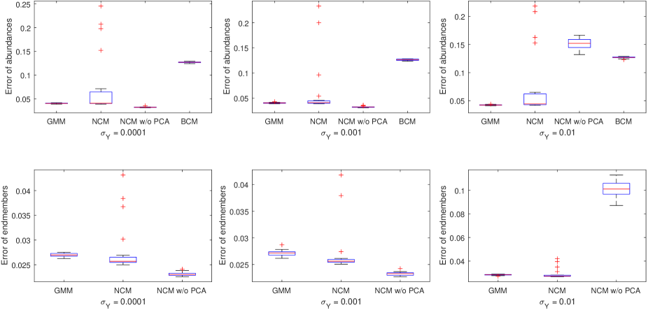
Figure 3: Abundance and endmember error statistics from 20 synthetic images for each noise level in the supervised unmixing scenario.

Unsupervised. We created two synthetic images in this case, the first was used to validate the ability to estimate the distribution parameters on scenes with regions of pure pixels, the second was used to validate the segmentation strategy on images with insufficient pure pixels. They were both of size $60\times 60$ pixels and constructed from 4 endmember classes: limestone, basalt, concrete, asphalt, whose spectral signatures were highly differentiable. We assumed that the endmembers were sampled from GMMs following the example in Section II-C. The means of the GMMs were from the ASTER spectral library [50] (see Fig. 4(c) for their spectra) with slight constant changes, which determined a spectral range from 0.4 $\mu$m to 14 $\mu$m, re-sampled into 200 values. The covariance matrices were constructed by $a_{jk}^{2}\mathbf{I}_{B}+b_{jk}^{2}\mathbf{u}_{jk}\mathbf{u}_{jk}^{T}$ where $\mathbf{u}_{jk}$ was a unit vector controlling the major variation direction. For the first image, we assumed the 4 materials occupied the 4 quadrants of the square image as pure pixels. Then Gaussian smoothing was applied on each abundance map to make the boundary pixels of each quadrant be mixed by the neighboring materials. For the second image, we made the first material as background, the other materials randomly placed on this background. The procedure of generating the abundance maps followed [37]: for each material (not as background), 150 Gaussian blobs were randomly placed, whose location and shape width were both sampled from Gaussian distributions. Finally, noise produced similar to above with $\sigma_{Y}=0.001$ was added to the generated pixels. Fig. 4 shows the abundance maps, the original spectra of these materials, and the resulting color images by extracting the bands corresponding to wavelengths 488 nm, 556 nm, 693 nm.

Figure 4: Unsupervised synthetic dataset. (a) and (b) are abundance maps for two images. (c) shows original spectra from the ASTER library. (d) and (e) show the color images.

The parameters of GMM were $r_{se}=5$ for the two images, $\beta_{1}=0.1$, $\beta_{2}=0.1$ for the second image. Fig. 5 shows the histograms of ground truth pure pixels and the estimated distributions for the first image. The ground truth distribution is barely visible as most of the time it coincides with GMM. For limestone and asphalt, all the distributions are similar since the pure pixels are generated by a unimodal Gaussian. However, for basalt and concrete, GMM provides a more accurate estimation while the two NCMs seem inferior due to the single Gaussian assumption. The quantitative analysis in Table II implies a similar result by calculating the $L_{2}$ distance between the estimated distribution and the ground truth.

Figure 5: Histograms of pure pixels for the 4 materials (when projected to a 1-dimensional space determined by performing PCA on the pure pixels of each material) and the ground truth and estimated distributions (also projected to the same direction) for the first image of the unsupervised synthetic dataset. The probability of each distribution is calculated by multiplying the value of the density function at each bin location with the bin size.

Table II: $L_{2}$ distance between the fitted distributions (GMM, NCM) and the ground truth distributions for the first image of the unsupervised synthetic dataset.

$\times 10^{6}$	Limestone	Basalt	Concrete	Asphalt	Mean
GMM	4.45	3.46	3.41	4.28	3.85
NCM	4.27	5.86	4.95	4.02	4.77

Table III shows the comparison of abundance errors from the two images. Since the second image is much more challenging than the first one, we can expect increased errors from all the methods. In general, the results of BCM and the two NCMs show slightly inferior abundances compared to GMM despite the fact that they have access to pure pixels in the image to train their models.

Table III: Abundance errors for the unsupervised synthetic dataset.

	$\times 10^{-4}$	GMM	NCM	NCM w/o PCA	BCM
Image 1	Limestone	50	107	92	126
	Basalt	40	74	67	158
	Concrete	41	66	62	186
	Asphalt	69	141	123	292
	Mean	59	97	86	190
Image 2	Limestone	157	1086	396	231
	Basalt	126	445	270	204
	Concrete	103	985	229	206
	Asphalt	225	170	706	445
	Mean	153	671	400	272

IV-B Pavia University

The Pavia University dataset was recorded by the Reflective Optics System Imaging Spectrometer (ROSIS) during a flight over Pavia, northern Italy. The dimension is 340 by 610 with a spatial resolution of 1.3 meters/pixel. It has 103 bands with wavelengths ranging from 430 nm to 860 nm. As Fig. 1 shows, the original image contains several man-made and natural materials. Considering that the whole dataset contains many different objects, we only performed experiments on the exemplar ROI (47 by 106) shown in Fig. 1, in which 5 endmembers, meadows, bare soil, painted metal sheets, shadows and pavement, are manually identified.

The parameter of GMM was $r_{se}=2$. Fig. 6 shows the GMM in the wavelength-reflectance space, where we can see the centers and the major variations of the Gaussians. Fig. 7 shows the scatter plot of the results in the projected space. The scatter plot shows that the identified Gaussian components cover the ground truth pure pixels very well. For painted metal sheets, which has a broad range of pure pixels, it estimated 4 components to cover them. For shadows, only one component was estimated. Fig. 8 shows the histograms of pure pixels and the estimated distributions of GMM and NCMs. We can see that GMM matches the background histogram better than NCMs.

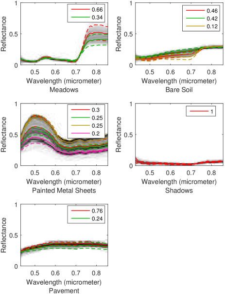
Figure 6: Estimated GMM in the wavelength-reflectance space for the Pavia University dataset. The background gray image represents the histogram created by placing the pure pixel spectra into the reflectance bins at each wavelength. The different colors represent different components, where the solid curve is the center $\boldsymbol{\mu}_{jk}$, the dashed curves are $\boldsymbol{\mu}_{jk}\pm 2\sigma_{jk}\mathbf{v}_{jk}$ ($\sigma_{jk}$ is the square root of the large eigenvalue of $\boldsymbol{\Sigma}_{jk}$ while $\mathbf{v}_{jk}$ is the corresponding eigenvector), and the legend shows the prior probabilities.

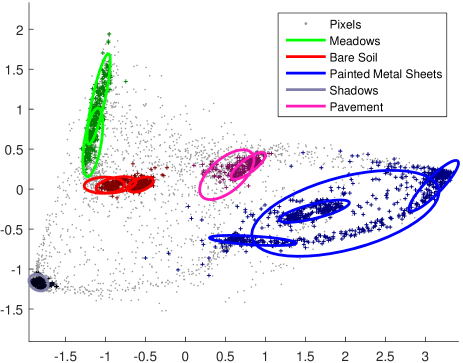
Figure 7: Scatter plot of the Pavia University dataset with the estimated GMM. The gray dots are the projected pixels by PCA. The darkened dots with a color represent the ground truth pure pixels for a material. The ellipses with the same color represent the projected Gaussian components (twice the standard deviation along the major and minor axes, covering 86% of the total probability mass) for one endmember.

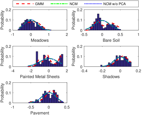
Figure 8: Histograms of pure pixels for the Pavia University dataset and the estimated distributions from GMM and NCM when projected to 1 dimension.

Fig. 9 shows the abundance map comparison. Comparing them with the ground truth shown in Fig. 1(a), we can see that BCM failed to estimate the pure pixels of painted metal sheets, although ground truth pure pixels were used for training. For example, the third and fourth abundance maps of BCM show that the pixels in the lower part of painted metal sheets are mixed with shadows, while the reduced reflectances are only caused by angle variation. The result of GMM not only shows sparse abundances for that region, but also interprets the boundary as a combination of neighboring materials. Since this dataset has a spatial spacing of 1.3 meters/pixel, we think this soft transition is more realistic than a simple segmentation. Although the results of NCMs look good in general, the abundances in a pure material region are inconsistent. The errors of abundances and endmembers for these algorithms are shown in Table IV, which implies that GMM performed best overall.

Figure 9: Abundance maps for the Pavia University dataset. The corresponding endmembers from left to right are meadows, bare soil, painted metal sheets, shadows and pavement.

Table IV: Abundance and endmember errors for Pavia University.

$\times 10^{-4}$	GMM	NCM	NCM w/o PCA	BCM
Meadow	187 \ 44a	405 \ 113	378 \ 114	711
Soil	175 \ 30	581 \ 68	507 \ 66	1049
Metal	476 \ 49	1236 \ 237	917 \ 349	1285
Shadow	44 \ 44	736 \ 48	914 \ 34	1287
Pavement	473 \ 39	1064 \ 114	333 \ 103	612
Mean	271 \ 41	804 \ 116	610 \ 133	989

• the numbers in ".\." denote the abundance and endmember errors.

IV-C Mississippi Gulfport

The dataset was collected over the University of Southern Mississippis-Gulfpark Campus [51]. It is a 271 by 284 image with 72 bands corresponding to wavelengths 0.368 $\mu m$ to 1.043 $\mu m$. The spatial resolution is 1 meter/pixel. The scene contains several man-made and natural materials including sidewalks, roads, various types of building roofs, concrete, shrubs, trees, and grasses. Since the scene contains many cloths for target detection, we tried to avoid the cloths and selected a 58 by 65 ROI that contains 5 materials [52]. The original RGB image and the selected ROI are shown in Fig. 10(a) while the identified materials and the mean spectra are shown in (b).

Figure 10: (a) Original RGB image of the Mississippi Gulfport dataset with selected ROI and (b) Ground truth materials in the ROI with their mean spectra.

The parameter of GMM was $r_{se}=1$. Fig. 11 shows the GMM result in the wavelength-reflectance space and Fig. 12 shows the scatter plot. We can see that the estimated Gaussian components successfully cover the identified pure pixels. Fig. 13 shows the estimated distributions. Although there are no multiple peaks in any of the histograms, NCMs still do not fit the histograms of shadow and gray roof. In contrast, GMM gives a much better fit for these 2 endmember distributions.

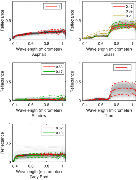
Figure 11: Estimated GMM in the wavelength-reflectance space for the Mississippi Gulfport dataset. The background gray image and the curves have the same meaning as in Fig. 6.

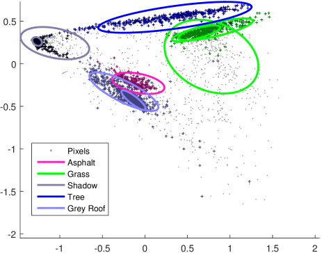
Figure 12: Scatter plot of the Mississippi Gulfport dataset with the estimated GMM. The ellipses and the dots have the same meaning as in Fig. 7.

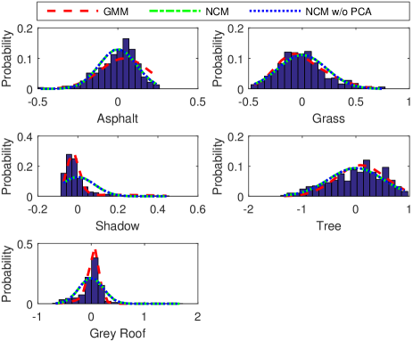
Figure 13: Histograms of pure pixels for the Gulfport dataset and the estimated distributions from GMM and NCM when projected to 1 dimension.

Fig. 14 shows the abundance maps from different algorithms. We can see that GMM matches the ground truth in Fig. 10(b) best, followed by NCM without PCA. This is also verified in the quantitative analysis in Table V. Although NCM and BCM take ground truth pure pixels as input, the scattered dots for trees (fourth abundance map) in both of them and the incomplete region of grass for NCM (asphalt for BCM) show their insufficiency in this case.

Figure 14: Abundance maps for the Gulfport dataset. The corresponding endmembers from left to right are asphalt, grass, shadow, tree and grey roof.

Table V: Abundance and endmember errors for the Gulfport dataset.

$\times 10^{-4}$	GMM	NCM	NCM w/o PCA	BCM
Asphalt	205 \ 52a	1693 \ 94	939 \ 59	1420
Grass	169 \ 58	1982 \ 121	558 \ 65	2145
Shadow	499 \ 49	1294 \ 68	921 \ 43	1315
Tree	1029 \ 89	2194 \ 234	1106 \ 185	2279
Roof	908 \ 76	2143 \ 174	1234 \ 104	1657
Mean	562 \ 65	1861 \ 138	952 \ 91	1763

• the numbers in ".\." denote the abundance and endmember errors.

V Discussion and Conclusion

In this paper, we introduced a GMM approach to represent endmember variability, by observing that the identified pure pixels in real applications usually can not be well fitted by a unimodal distribution as in NCM or BCM. We solved several obstacles in linear unmixing using this distribution, including (i) deriving the conditional probability density function of the mixed pixel given each endmember modeled as GMM from two perspectives; (ii) estimating the abundances and endmember distributions by maximizing the log-likelihood with a prior enforcing abundance smoothness and sparsity; (iii) estimating the endmembers for each pixel given the abundances and distribution parameters. The results on synthetic and real datasets show superior accuracy compared to current popular methods like NCM, BCM. Here we have some final remarks.

Complexity. As analyzed in Section III-F, each iteration in the estimation of abundances has spatial complexity $O\left(\left|\mathcal{K}\right|NB^{2}\right)$ and time complexity $O\left(\left|\mathcal{K}\right|NB^{3}\right)$. For comparison, the implemented NCM has the same complexity but with $\left|\mathcal{K}\right|=1$. For the supervised synthetic dataset which contains 60 images, the total running time of GMM was 9709 seconds, on a desktop with a Intel Core i7-3820 CPU and 64 GB memory. For comparison, the running time of NCM, NCM without PCA, and BCM was 941, 50751, 62525 seconds respectively. In real applications, running GMM on the Pavia University and Mississippi Gulfport ROIs required 734 seconds and 97 seconds respectively for abundance estimation (24 seconds and 17 seconds for endmember estimation), compared to 40 and 34 seconds from NCM, 1389 and 396 seconds from NCM without PCA, 1170 and 616 seconds from BCM. As analyzed, the main factors affecting the efficiency of GMM and NCMs are $\left|\mathcal{K}\right|$ and $B$.

Limitation. The complexity analysis leads to one limitation of the method. That is, the complexity grows exponentially with increasing numbers of components. This could cause problems for a large amount of pure pixels. To overcome this shortcoming, there are some empirical workarounds, such as reducing the number of components by introducing thresholds, or reducing the number of pure pixels to a fixed number by random sampling. Another limitation is that the proposed unsupervised version assumes presence of regions of pure pixels, which mostly happens in urban scenes. For scenes with a lot of mixed pixels, this assumption may not hold. Note that unsupervised unmixing is a very challenging problem. The previous works for this problem all assume several properties on the abundances and endmembers [21, 22, 23]. Hence, this limitation exists more or less in all the works on this problem. Finally, the method was only evaluated on real urban datasets with only ground truth on pure pixels: it is therefore unclear if the abundance estimation on mixed pixels is also accurate. This is due to lack of datasets and ground truth in the hyperspectral community. We plan to validate it on a more comprehensive dataset given in [31] in the future.

Future work. The proposed GMM formulation has several applications that we can investigate in the future. First, in target detection, endmember variability may interfere with the target as well as the background [53]. By modeling the target or the background as spectra sampled from GMM distributions, we may devise more sophisticated and accurate target detection algorithms. Second, in fusion of hyperspectral and multispectral images, the LMM is usually used to overcome the underdetermined nature of the problem [54, 55]. However, the LMM does not hold in real scenarios as shown in this work. If we use the LMM with endmember variability, which is modeled by samples from GMM distributions, we may have a fusion algorithm that better fits the data. Finally, in estimating the noise or intrinsic dimension of hyperspectral images, simulated data are generated to quantify the results [46]. When these simulated data are created, usually the LMM is used without considering the endmember variability. Using the GMM formulation, we may generate distinct endmembers for each pixel and create more realistic synthetic data.

Yuan Zhou received the B.E degree in Software Engineering (2008), the M.E. degree in Computer Application Technology (2011), both from Huazhong University of Science and Technology, Wuhan, Hubei, China. Then he worked in Shanghai UIH as a software engineer for two years. Since 2013, he has been a Ph.D. student in the Department of CISE, University of Florida, Gainesville, FL, USA. His research interests include image processing, computer vision and machine learning.

Anand Rangarajan is in the Department of Computer and Information Science and Engineering, University of Florida, Gainesville, FL, USA. His research interests are machine learning, computer vision and the scientific study of consciousness.

Paul Gader (M’86–SM’09–F’11) received the Ph.D. degree in mathematics for image-processing-related research from the University of Florida, Gainesville, FL, USA, in 1986. He was a Senior Research Scientist with Honeywell, a Research Engineer and a Manager with the Environmental Research Institute of Michigan, Ann Arbor, MI, USA, and a Faculty Member with the University of Wisconsin, Oshkosh, WI, USA, the University of Missouri, Columbia, MO, USA, and the University of Florida, FL, USA, where he is currently a Professor of Computer and Information Science and Engineering. He performed his first research in image processing in 1984 working on algorithms for the detection of bridges in forward-looking infrared imagery as a Summer Student Fellow at Eglin Air Force Base. He has since worked on a wide variety of theoretical and applied research problems including fast computing with linear algebra, mathematical morphology, fuzzy sets, Bayesian methods, handwriting recognition, automatic target recognition, biomedical image analysis, landmine detection, human geography, and hyperspectral and light detection, and ranging image analysis projects. He has authored/co-authored hundreds of refereed journal and conference papers.

References

- [1] M. Berman, H. Kiiveri, R. Lagerstrom, A. Ernst, R. Dunne, and J. F. Huntington, “ICE: A statistical approach to identifying endmembers in hyperspectral images,” IEEE Trans. on Geoscience and Remote Sensing, vol. 42, no. 10, pp. 2085–2095, 2004.
- [2] J. M. Nascimento and J. M. Bioucas Dias, “Vertex component analysis: A fast algorithm to unmix hyperspectral data,” IEEE Trans. on Geoscience and Remote Sensing, vol. 43, no. 4, pp. 898–910, 2005.
- [3] A. Zare, P. D. Gader, O. Bchir, and H. Frigui, “Piecewise convex multiple-model endmember detection and spectral unmixing,” IEEE Trans. on Geoscience and Remote Sensing, vol. 51, no. 5, pp. 2853–2862, 2013.
- [4] J. M. Bioucas-Dias, A. Plaza, N. Dobigeon, M. Parente, Q. Du, P. D. Gader, and J. Chanussot, “Hyperspectral unmixing overview: Geometrical, statistical, and sparse regression-based approaches,” IEEE Journal of Selected Topics in Applied Earth Observations and Remote Sensing, vol. 5, no. 2, pp. 354–379, 2012.
- [5] N. Keshava and J. F. Mustard, “Spectral unmixing,” IEEE Signal Processing Magazine, vol. 19, no. 1, pp. 44–57, 2002.
- [6] B. Hapke, “Bidirectional reflectance spectroscopy: 1. theory,” Journal of Geophysical Research: Solid Earth (1978–2012), vol. 86, no. B4, pp. 3039–3054, 1981.
- [7] A. Halimi, Y. Altmann, N. Dobigeon, and J.-Y. Tourneret, “Nonlinear unmixing of hyperspectral images using a generalized bilinear model,” IEEE Trans. on Geoscience and Remote Sensing, vol. 49, no. 11, pp. 4153–4162, 2011.
- [8] B. Somers, K. Cools, S. Delalieux, J. Stuckens, D. Van der Zande, W. W. Verstraeten, and P. Coppin, “Nonlinear hyperspectral mixture analysis for tree cover estimates in orchards,” Remote Sensing of Environment, vol. 113, no. 6, pp. 1183–1193, 2009.
- [9] R. Heylen and P. D. Gader, “Nonlinear spectral unmixing with a linear mixture of intimate mixtures model,” IEEE Geoscience and Remote Sensing Letters, vol. 11, no. 7, pp. 1195–1199, 2014.
- [10] J. Broadwater and A. Banerjee, “A generalized kernel for areal and intimate mixtures,” in 2nd Workshop on Hyperspectral Image and Signal Processing: Evolution in Remote Sensing (WHISPERS). IEEE, 2010, pp. 1–4.
- [11] J. Broadwater, R. Chellappa, A. Banerjee, and P. Burlina, “Kernel fully constrained least squares abundance estimates,” in IEEE International Geoscience and Remote Sensing Symposium (IGARSS). IEEE, 2007, pp. 4041–4044.
- [12] R. Heylen, M. Parente, and P. D. Gader, “A review of nonlinear hyperspectral unmixing methods,” IEEE Journal of Selected Topics in Applied Earth Observations and Remote Sensing, vol. 7, no. 6, pp. 1844–1868, 2014.
- [13] B. Somers, G. P. Asner, L. Tits, and P. Coppin, “Endmember variability in spectral mixture analysis: A review,” Remote Sensing of Environment, vol. 115, no. 7, pp. 1603–1616, 2011.
- [14] A. Zare and K. Ho, “Endmember variability in hyperspectral analysis: Addressing spectral variability during spectral unmixing,” IEEE Signal Processing Magazine, vol. 31, no. 1, pp. 95–104, 2014.
- [15] X. Du, A. Zare, P. D. Gader, and D. Dranishnikov, “Spatial and spectral unmixing using the Beta compositional model,” IEEE Journal of Selected Topics in Applied Earth Observations and Remote Sensing, vol. 7, no. 6, pp. 1994–2003, 2014.
- [16] A. Zare and P. D. Gader, “PCE: Piecewise convex endmember detection,” IEEE Trans. on Geoscience and Remote Sensing, vol. 48, no. 6, pp. 2620–2632, 2010.
- [17] D. A. Roberts, M. Gardner, R. Church, S. Ustin, G. Scheer, and R. Green, “Mapping chaparral in the Santa Monica Mountains using multiple endmember spectral mixture models,” Remote Sensing of Environment, vol. 65, no. 3, pp. 267–279, 1998.
- [18] A. Halimi, N. Dobigeon, and J.-Y. Tourneret, “Unsupervised unmixing of hyperspectral images accounting for endmember variability,” IEEE Trans. on Image Processing, vol. 24, no. 12, pp. 4904–4917, 2015.
- [19] O. Eches, N. Dobigeon, C. Mailhes, and J.-Y. Tourneret, “Bayesian estimation of linear mixtures using the normal compositional model: Application to hyperspectral imagery,” IEEE Trans. on Image Processing, vol. 19, no. 6, pp. 1403–1413, 2010.
- [20] C. A. Bateson, G. P. Asner, and C. A. Wessman, “Endmember bundles: A new approach to incorporating endmember variability into spectral mixture analysis,” IEEE Trans. on Geoscience and Remote Sensing, vol. 38, no. 2, pp. 1083–1094, 2000.
- [21] L. Drumetz, M.-A. Veganzones, S. Henrot, R. Phlypo, J. Chanussot, and C. Jutten, “Blind hyperspectral unmixing using an extended linear mixing model to address spectral variability,” IEEE Transactions on Image Processing, vol. 25, no. 8, pp. 3890–3905, 2016.
- [22] P.-A. Thouvenin, N. Dobigeon, and J.-Y. Tourneret, “Hyperspectral unmixing with spectral variability using a perturbed linear mixing model,” IEEE Transactions on Signal Processing, vol. 64, no. 2, pp. 525–538, 2016.
- [23] A. Halimi, P. Honeine, and J. M. Bioucas-Dias, “Hyperspectral unmixing in presence of endmember variability, nonlinearity, or mismodeling effects,” IEEE Transactions on Image Processing, vol. 25, no. 10, pp. 4565–4579, 2016.
- [24] B. Zhang, L. Zhuang, L. Gao, W. Luo, Q. Ran, and Q. Du, “PSO-EM: A hyperspectral unmixing algorithm based on normal compositional model,” IEEE Trans. on Geoscience and Remote Sensing, vol. 52, no. 12, pp. 7782–7792, 2014.
- [25] O. Eches, N. Dobigeon, and J.-Y. Tourneret, “Estimating the number of endmembers in hyperspectral images using the normal compositional model and a hierarchical Bayesian algorithm,” IEEE Journal of Selected Topics in Signal Processing, vol. 4, no. 3, pp. 582–591, 2010.
- [26] C. Song, “Spectral mixture analysis for subpixel vegetation fractions in the urban environment: How to incorporate endmember variability?,” Remote Sensing of Environment, vol. 95, no. 2, pp. 248–263, 2005.
- [27] J.-P. Combe, S. Le Mouelic, C. Sotin, A. Gendrin, J. Mustard, L. Le Deit, P. Launeau, J.-P. Bibring, B. Gondet, Y. Langevin, et al., “Analysis of omega/mars express data hyperspectral data using a multiple-endmember linear spectral unmixing model (melsum): Methodology and first results,” Planetary and Space Science, vol. 56, no. 7, pp. 951–975, 2008.
- [28] G. P. Asner and D. B. Lobell, “A biogeophysical approach for automated SWIR unmixing of soils and vegetation,” Remote sensing of environment, vol. 74, no. 1, pp. 99–112, 2000.
- [29] G. P. Asner and K. B. Heidebrecht, “Spectral unmixing of vegetation, soil and dry carbon cover in arid regions: comparing multispectral and hyperspectral observations,” International Journal of Remote Sensing, vol. 23, no. 19, pp. 3939–3958, 2002.
- [30] A. Castrodad, Z. Xing, J. B. Greer, E. Bosch, L. Carin, and G. Sapiro, “Learning discriminative sparse representations for modeling, source separation, and mapping of hyperspectral imagery,” IEEE Transactions on Geoscience and Remote Sensing, vol. 49, no. 11, pp. 4263–4281, 2011.
- [31] E. B. Wetherley, D. A. Roberts, and J. P. McFadden, “Mapping spectrally similar urban materials at sub-pixel scales,” Remote Sensing of Environment, vol. 195, pp. 170–183, 2017.
- [32] D. Stein, “Application of the normal compositional model to the analysis of hyperspectral imagery,” in IEEE Workshop on Advances in Techniques for Analysis of Remotely Sensed Data, 2003, pp. 44–51.
- [33] L. Tits, B. Somers, and P. Coppin, “The potential and limitations of a clustering approach for the improved efficiency of multiple endmember spectral mixture analysis in plant production system monitoring,” IEEE Transactions on Geoscience and Remote Sensing, vol. 50, no. 6, pp. 2273–2286, 2012.
- [34] M.-D. Iordache, L. Tits, J. M. Bioucas-Dias, A. Plaza, and B. Somers, “A dynamic unmixing framework for plant production system monitoring,” IEEE Journal of Selected Topics in Applied Earth Observations and Remote Sensing, vol. 7, no. 6, pp. 2016–2034, 2014.
- [35] L. Tits, B. Somers, W. Saeys, and P. Coppin, “Site-specific plant condition monitoring through hyperspectral alternating least squares unmixing,” IEEE Journal of Selected Topics in Applied Earth Observations and Remote Sensing, vol. 7, no. 8, pp. 3606–3618, 2014.
- [36] J. B. Lee, A. S. Woodyatt, and M. Berman, “Enhancement of high spectral resolution remote-sensing data by a noise-adjusted principal components transform,” IEEE Transactions on Geoscience and Remote Sensing, vol. 28, no. 3, pp. 295–304, 1990.
- [37] Y. Zhou, A. Rangarajan, and P. D. Gader, “A spatial compositional model for linear unmixing and endmember uncertainty estimation,” IEEE Trans. on Image Processing, vol. 25, no. 12, pp. 5987–6002, 2016.
- [38] D. Achlioptas and F. McSherry, “On spectral learning of mixtures of distributions,” in Learning Theory, pp. 458–469. Springer, 2005.
- [39] N. Vlassis and A. Likas, “A greedy EM algorithm for gaussian mixture learning,” Neural Processing Letters, vol. 15, no. 1, pp. 77–87, 2002.
- [40] K. Lange, Optimization, Springer, 2013.
- [41] X.-L. Meng and D. B. Rubin, “Maximum likelihood estimation via the ECM algorithm: A general framework,” Biometrika, vol. 80, no. 2, pp. 267–278, 1993.
- [42] D. P. Bertsekas, Nonlinear programming, Athena Scientific, 1999.
- [43] C.-J. Lin, “Projected gradient methods for nonnegative matrix factorization,” Neural Computation, vol. 19, no. 10, pp. 2756–2779, 2007.
- [44] G. J. McLachlan and S. Rathnayake, “On the number of components in a Gaussian mixture model,” Wiley Interdisciplinary Reviews: Data Mining and Knowledge Discovery, vol. 4, no. 5, pp. 341–355, 2014.
- [45] P. Smyth, “Model selection for probabilistic clustering using cross-validated likelihood,” Statistics and Computing, vol. 10, no. 1, pp. 63–72, 2000.
- [46] L. Gao, Q. Du, B. Zhang, W. Yang, and Y. Wu, “A comparative study on linear regression-based noise estimation for hyperspectral imagery,” IEEE Journal of Selected Topics in Applied Earth Observations and Remote Sensing, vol. 6, no. 2, pp. 488–498, 2013.
- [47] R. Roger, “Principal components transform with simple, automatic noise adjustment,” International Journal of Remote Sensing, vol. 17, no. 14, pp. 2719–2727, 1996.
- [48] N. Guan, D. Tao, Z. Luo, and B. Yuan, “Manifold regularized discriminative nonnegative matrix factorization with fast gradient descent,” IEEE Trans. on Image Processing, vol. 20, no. 7, pp. 2030–2048, 2011.
- [49] C. M. Bishop, Pattern recognition and machine learning, springer New York, 2006.
- [50] A. Baldridge, S. Hook, C. Grove, and G. Rivera, “The ASTER spectral library version 2.0,” Remote Sensing of Environment, vol. 113, no. 4, pp. 711–715, 2009.
- [51] P. Gader, A. Zare, R. Close, J. Aitken, and G. Tuell, “MUUFL Gulfport hyperspectral and LiDAR airborne data set,” Tech. Rep. REP-2013-570, Univ. Florida, Gainesville, FL, USA, 2013.
- [52] X. Du and A. Zare, “Technical report: Scene label ground truth map for MUUFL Gulfport data set,” Tech. Rep. 20170417, Univ. Florida, Gainesville, FL, USA, 2017.
- [53] C. Jiao and A. Zare, “Functions of multiple instances for learning target signatures,” IEEE Transactions on Geoscience and Remote Sensing, vol. 53, no. 8, pp. 4670–4686, 2015.
- [54] N. Yokoya, T. Yairi, and A. Iwasaki, “Coupled nonnegative matrix factorization unmixing for hyperspectral and multispectral data fusion,” IEEE Transactions on Geoscience and Remote Sensing, vol. 50, no. 2, pp. 528–537, 2012.
- [55] Q. Wei, N. Dobigeon, and J.-Y. Tourneret, “Fast fusion of multi-band images based on solving a sylvester equation,” IEEE Transactions on Image Processing, vol. 24, no. 11, pp. 4109–4121, 2015.