Revealing Fine Structure in the Antineutrino Spectra From a Nuclear Reactor

Abstract

We calculate the Inverse Beta Decay (IBD) antineutrino spectrum generated by nuclear reactors using the summation method to understand deviations from the smooth Huber-Mueller model due to the decay of individual fission products, showing that plotting the ratio of two adjacent spectra points can effectively reveal these deviations. We obtained that for binning energies of 0.1 MeV or lower, abrupt changes in the spectra due to the jagged nature of the individual antineutrino spectra could be observed for highly precise experiments. Surprisingly, our calculations also reveal a peak-like feature in the adjacent points ratio plot at 4.5 MeV even with a 0.25 MeV binning interval, which we find is present in the IBD spectrum published by Daya Bay in 2016. We show that this 4.5 MeV feature is caused by the contributions of just four fission products, ⁹⁵Y, ^98,101Nb and ¹⁰²Tc. This would be the first evidence of the decay of a few fission products in the IBD antineutrino spectrum from a nuclear reactor.

Since the discovery of radioactivity in 1895 becquerel96 , scientists have been able to accurately characterize the $\gamma$, e^-, e⁺, neutron, proton and $\alpha$ spectra emitted by nuclei during their radioactive decay. However, measuring the antineutrino spectra from the decay of individual nuclei has eluded experimental efforts even today as antineutrinos only interact with matter through the weak interaction. The closest direct measurements of neutrino spectra following beta-decay are the neutrino oscillation measurements of the SNO experiment sno which measured neutrinos following solar ⁸B decay. However, the energy distribution of antineutrinos from a single nucleus following $\beta$-minus decay has not been reported to the best of our knowledge. There has been, however, tremendous success in detecting antineutrinos from nuclear reactors, starting with the pioneering work of Cowan and Reines cowan56 . Most recently, the Daya Bay dayabay16 , Double Chooz doublechooz , and RENO reno16 collaborations have measured reactor’s antineutrino spectra with unprecedented statistics by placing large antineutrino detectors in the vicinity of commercial reactors. In these experiments, antineutrinos are produced by the approximately 800 fission products, and are later detected through the use of the Inverse Beta Decay (IBD) reaction, $\overline{\nu}_{e}+p\rightarrow n+e^{+}$. Since the IBD cross section increases steadily for energies above its 1.8 MeV threshold, and as the antineutrino spectrum generated by a reactor decreases with increasing energy, the resulting IBD spectrum has a bell shape with the maximum around 3.5-4.0 MeV.

The focus in the interpretation and understanding of these reactor experiments has been through comparing the integral and overall shape of the measured spectrum to various predictions. Currently, the antineutrino spectra from Huber huber11 for ²³⁵U, ²³⁹Pu and ²⁴¹Pu, obtained from converting measured aggregate electron spectra ill82 ; ill85 ; ill89 , and that of Mueller et al. mueller11 for ²³⁸U derived from nuclear databases, are thought to be the best predictions. Comparisons of measured IBD spectra with the Huber-Mueller model have led to the observation of an overall deficit in the number of measured antineutrinos along with a spectra distortion mention11 . These findings then spurred a flurry of investigations into the source of these disagreements hayes14 ; hayes15 ; huber17 ; dayabay17 ; sonzogni17 ; mention17 .

To study the possible existence of sterile neutrinos, as well as to gauge antineutrinos’ potential to monitor nuclear reactors christensen14 , a new generation of experiments at very short baselines prospect ; nucifer ; neos17 have begun or will soon begin to collect data near a reactor core. In particular, the NEOS collaboration neos17 recently published their IBD spectrum with a binning interval of 0.1 MeV, that is, a considerable improvement over the 0.25 MeV value that has been the standard so far. The presence of deviations in the NEOS IBD spectrum from the Huber-Mueller predictions near the maximum was the initial motivation for this work, where we explore the possibility of observing signatures of the individual fission products amidst the overall spectrum, which in vague analogy with other radiation types, we will refer to as “fine structure”. In an attempt to view the trees out of the forest, we present a novel approach to analyzing antineutrino spectra which involves taking ratios of adjacent energy bins. We then apply this technique to the highest resolution data available from the Daya Bay collaboration and find that even with a 0.25 MeV binning, discontinuities in the antineutrino spectra are evident and moreover, are in agreement with calculations which consider the decay of all fission fragments produced in the reactor. These discontinuities can be attributed to just a few nuclei, suggesting that indeed the individual signatures of the fission fragments can be unraveled from the whole.

Electrons and antineutrinos are produced in a nuclear reactor following the $\beta-$ decay of neutron rich fission products, whose spectra can be calculated using the summation method vogel81 as

$$S(E)=\sum_{i}\sum_{j}f_{i}\times CFY_{ij}\times S_{j}(E),$$ (1)

where $f_{i}$ are the effective fission fractions for the four main fuel components, ²³⁵U, ²³⁸U, ²³⁹Pu and ²⁴¹Pu; $CFY_{ij}$ are the cumulative fission yields from the neutron induced fission on these fissile nuclides; and the spectra $S_{j}(E)$ are calculated as

$$S_{j}(E)=\sum I_{jk}\times S_{jk}(E),$$ (2)

with $I_{jk}$ the $\beta-$ decay intensity from the jth $\beta$-minus decaying level in the network to the kth level in the daughter nucleus, and $S_{jk}(E)$ are the corresponding nuclear level to nuclear level spectra, which for electrons are given by

$$\begin{split}S(E)=&N\times W\times(W^{2}-1)^{1/2}\times(W-W_{0})^{2}\times\\ &F(Z,W)\times C(Z,W),\end{split}$$ (3)

where N is a constant so that $S(E)$ is normalized to unity; $W$ is the relativistic kinetic energy, $W=E/m_{e}c^{2}+1$, and $W_{0}$=$Q/m_{e}c^{2}+1$, with $Q$ the total decay energy available also known as the end-point energy; $F(Z,W)$ is the Fermi function and $Z$ is the number of protons in the daughter nucleus; lastly, the $C(Z,W)$ term contains the corrections due to angular momentum and parity changes, finite size, screening, radiative and weak magnetism.

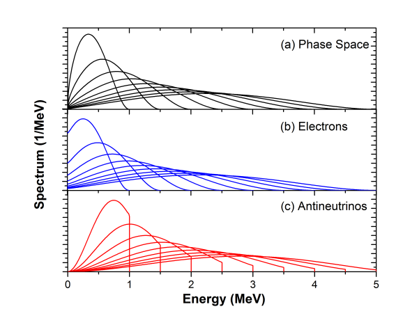
Figure 1: (a) Energy distribution using only the phase space term, (b) energy distribution for electrons including all the correction terms (c) as the middle panel but for antineutrinos.

The $W\times(W^{2}-1)^{1/2}\times(W-W_{0})^{2}$ product in Eq. (3) is colloquially known as the “phase space” term as it is customarily inferred using statistical classical mechanics arguments. In the absence of Coulomb effects, the electron and antineutrino spectra would be given by this term, resulting in identical energy distributions, as seen in Fig. 1 (a). The presence of the Coulomb field generated by the protons in the nucleus gives rise to the Fermi function term, F(Z,W), which slows down the electrons. Conservation of energy then dictates a corresponding boost to the antineutrino energy. The effect for electrons can be seen in Fig. 1 (b), while the bottom panel shows the antineutrino spectra. Because of the Fermi function, the level-to-level antineutrino spectra exhibit an abrupt cutoff at the end-point energy. As a consequence, while a sum of electron spectra will have a smooth quality, a sum of antineutrino spectra may have a rugged, serrated nature. Fig. 1 also reveals that the cut-off in the antineutrino spectrum is more severe for lower-energy antineutrinos, being particularly pronounced for end point energies between 1 and 3 MeV, and with increasing end point energy the serrated portion of the spectrum quickly diminishes.

Producing a neutron-rich source of a single isotope, strong enough to observe the intriguing features in Fig. 1 (c), would be experimentally extremely challenging. The question is, within the 800 fission fragments (with 10 to 100’s of $\beta$ branches) produced in a nuclear reactor, can the spectra from individual nuclei be disentangled. We explore this possibility by calculating the antineutrino spectra for the Daya Bay experiment with the summation method using: (a) Daya Bay fission fractions dayabay16 ; (b) JEFF-3.1 fission yields jeff31 and updated ENDF/B-VII.1 decay data e71 as described in Refs. sonzogni15 ; sonzogni16 ; (c) $F(Z,W)$ and $C(Z,W)$ obtained as described by Huber huber11 ; (d) IBD cross sections from Ref. xs . The resulting IBD antineutrino spectrum is shown in Fig. 2(a), plotted together for contrast with the corresponding Huber-Mueller spectra (shifted down). The energy range was restricted to 2.5 to 5.5 MeV, where statistical uncertainties will be sufficiently low to allow the observation of fine structure.

Hints of fine structure begin to materialize in the summation calculation starting around 2.8 MeV; the most obvious is a sharp cutoff just below 3.5 MeV, which corresponds to the sharp cutoffs seen in Fig. 1(c). There is also another type of structure that spans several hundreds of keV, such as a shoulder around 4.2 to 4.5 MeV, which would correspond to the contribution of a single fission product or a group of them that have similar end point energies. The effect of binning in our summation calculations, not including experimental resolution effects, is explored in Fig. 2 (b), where with 0.25 MeV binning intervals, the standard one so far for Daya Bay, deviations from a smooth curve would be hard to discern by eyesight, while with 0.10 MeV bins, as available with the recent NEOS data neos17 , fine structure begins to manifest, and would become considerably clearer with a 0.05 keV binning. A similar analysis as a function of the detector resolution was presented in Ref. dwyer15 .

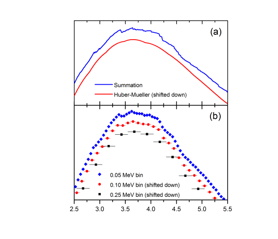
Figure 2: (a) Calculated Daya Bay IBD antineutrino spectra using the summation method (top blue line) and the Huber-Mueller antineutrino spectra (lower red line), shifted down to highlight the jaggedness of the former versus the smoothness of the latter. (b) IBD antineutrino spectra from summation calculations binned in 0.05, 0.10 and 0.25 MeV intervals. For contrast reasons, the last two curves are shifted down; additionally, experimental resolution effects were not included.

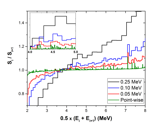
Figure 3: Ratio of two consecutive summation IBD spectrum points under different binning conditions. A zoom in the 4 to 5 MeV region can be seen in the top-left corner inset.

While there are definite features in the spectra shown in Fig. 2, they are difficult to interpret quantitatively. To better elucidate fine structure features, we consider the ratio between two adjacent points

$$R_{i}=S_{i}/S_{i+1},$$ (4)

as a function of the average bin interval $0.5\times(E_{i}+E_{i+1})$, which are plotted in Fig. 3 for a summation calculation IBD spectrum, under different binning scenarios. For a point-wise calculation, the sudden drop in the spectrum due to the abrupt end of a relevant fission product antineutrino spectrum would manifest as a peak, for instance that of ⁹⁶Y at 7.1 MeV, whose signature can also be seen with 0.05 and 0.1 MeV binning. Intuitively, it may be thought that for a 0.25 MeV binning, a smooth curve would be obtained. However, a peak-like feature around 4.5 MeV is visible, which as the inset in the top-left corner reveals, it is caused by a number of strong transitions that coincidentally have similar end-point energies. Inspired by this observation, the Daya Bay $R_{i}$ values are plotted in Fig. 4, where the uncertainties on $R_{i}$ were calculated using a first order Taylor expansion

$$\begin{split}\Delta^{2}R_{i}=&S^{-2}_{i+1}\times\sigma_{i,i}+S^{2}_{i}\times S^{-4}_{i+1}\times\sigma_{i+1,i+1}\\ &-2\times S_{i}\times S^{-3}_{i+1}\times\sigma_{i,i+1},\end{split}$$ (5)

with $\sigma$ the covariance matrix as given by the Daya Bay Collaboration dayabay16 . The need of the covariance matrix is significant here since as the adjacent $S_{i}$ points are positively correlated, that is $\sigma_{i+1,i+1}>0$, the $\Delta R_{i}$ values are smaller than those obtained assuming no correlation, which allows for a positive identification of the structures in the $R_{i}$ plot.

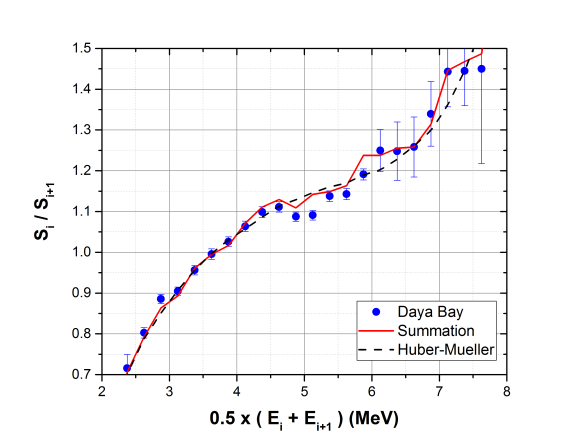
Figure 4: Ratio of two consecutive IBD spectrum points from the Daya Bay experiment (symbols), Huber-Mueller model (dashed black line) and summation method (full red line). For clarity’s sake, the calculated points are connected with a straight line, instead of a step function as in Fig. 3.

While the summation calculation $\chi^{2}$ per point in Fig. 4 is only marginally smaller than the corresponding Huber-Mueller $\chi^{2}$, the summation calculation shape is remarkably more similar to the experimental one. This demonstrates the necessity to improve the summation method, which despite being less precise than the conversion method due to deficiencies in fission yield and decay data fallot12 , is absolutely needed to fully understand the features of a reactor antineutrino spectrum.

The next question is if can we attribute the 4.5 MeV peak-like feature to individual nuclei. To answer this question, we searched for the most relevant individual IBD spectra with large $R$ values in the 4 to 5 MeV region. We find that the feature at 4.5 MeV is caused by just four nuclides, ⁹⁵Y, ^98,101Nb, and ¹⁰²Tc, which have in common large cumulative fission yields and antineutrino spectra dominated by strong transitions with end-point energy near 4.5 MeV. To understand why the number is so low, we need to remember that due to the double-humped nature of independent fission yield distributions, there is a relatively small number of nuclides with significant effective cumulative fission yields, $CFY_{eff,i}=\sum f_{k}CFY_{ki}$. For instance, for Daya Bay fission fractions, the largest effective CFY for products contributing to the IBD spectrum is that of ¹³⁴I with $CFY_{eff,i}$=0.073, and while the number of nuclides with effective CFYs larger than 0.01 is about 115, it drops to about 30 for effective CFYs larger than 0.05. This number is further reduced when we require these nuclides to have large values of $I_{ki}$ with end-point energies in the 4 to 5 MeV region. Fig. 5 (a) shows the total IBD spectrum, the one generated by the four nuclides in question, and the difference. These four nuclides account for about 6% of the total IBD antineutrino yield, and about 9.6% of the IBD antineutrino yield in the 1.8 to 4.5 MeV region. Fig. 5 (b) shows a plot of $R_{i}$ values with a 0.25 MeV binning with and without the contribution of ⁹⁵Y, ^98,101Nb, and ¹⁰²Tc, which clearly shows that the feature at 4.5 MeV is basically caused by these four nuclides.

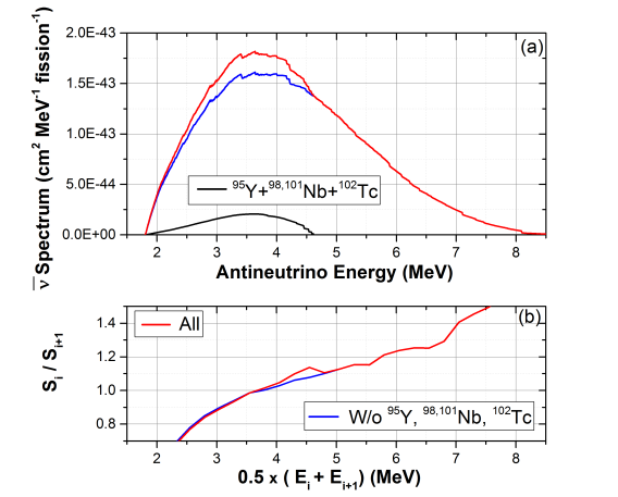
Figure 5: (a) Calculated Daya Bay IBD antineutrino spectra from all the fission products (red line), the ⁹⁵Y, ^98,101Nb, and ¹⁰²Tc contribution (black line), and the difference (blue line). (b) Corresponding ratio of two adjacent points with a 0.25 MeV binning.

As several prior works have investigated the need of reliable decay and fission yield data fallot12 ; sonzogni15 ; rasco16 to accurately calculate antineutrino spectra, we now assess the quality of the ⁹⁵Y, ^98,101Nb, and ¹⁰²Tc data to determine if the 4.5 MeV structure in the summation calculations is a solid prediction. The effective JEFF CFYs for these nuclides, with their relative uncertainty in parenthesis, are 0.058 (0.9%), 0.057 (3.4%), 0.054 (1.9%), and 0.050 (3.7%) respectively. The ENDF/B-VII.1 effective cumulative fission yields are similar, within 2% or less from the JEFF values, with the exception of ¹⁰²Tc, whose independent fission yield is considerably smaller than its cumulative as it is mainly produced in the decay of ¹⁰²Mo. When the ENDF/B yields were obtained, it was assumed that the isomer would take most of the $\beta$-decay intensity, which as we know today it is not the case. When this correction is applied, both values of cumulative fission yields agree very well. A look at the decay data used in our calculations reveals that for these four nuclides, the $\beta$ intensity pattern is dominated by a strong ground state (GS) to ground state transition with end point energies near 4.5 MeV. For instance, GS to GS transitions intensities and Q-values are: 64$\pm$1.7% and 4.45 MeV for ⁹⁵Y a95 , 57$\pm$7% and 4.59 MeV for ⁹⁸Nb a98 , 40$\pm$13% and 4.55 MeV for ¹⁰¹Nb a101 , 92.9$\pm$0.6% and 4.53 MeV for ¹⁰²Tc a102 ; jordan13 . We conclude that the nuclear data for these four nuclides are fairly reliable due to the relative closeness to the valley of stability.

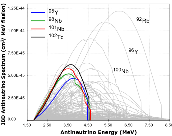
Figure 6: Calculated IBD antineutrino spectra from all the fission products, highlighting the ⁹⁵Y, ^98,101Nb, and ¹⁰²Tc ones.

Further insights can be obtained by studying Fig. 6, where the IBD antineutrino spectra for all the fission products are plotted, highlighting in particular the ⁹⁵Y, ^98,101Nb and ¹⁰²Tc ones, whose sum spectrum, due to the similarity of the end-point energies, effectively looks like that of a single strongly produced fission product. As a comparison, the three large spectra observed on the right side of the plot are, in descending order, those from ⁹²Rb, ⁹⁶Y and ¹⁰⁰Nb, which contribute about 6.7%, 5.3% and 4.1% to the total IBD antineutrino yield, respectively. Despite their sizable contribution, observing the fine structure caused by their antineutrino spectra sharp cutoff would be considerably more difficult as the relative importance of the sharp cutoff diminishes and the IBD antineutrino spectrum is considerably smaller at energies close to their end-point energies.

In summary, we have shown that as the IBD antineutrino spectrum from a nuclear reactor is the sum of about 800 fission products, there will be deviations from a smooth shape due to (a) the contribution of a strongly populated fission product, (b) sharp cutoffs in the individual antineutrino spectra, and (c) the contribution from a small number of fission products with similar end-point energy, effectively mimicking the first case. We developed a novel, yet simple way of numerically revealing these contributions, by plotting the ratio of adjacent points. We conclude that with a binning interval of 0.1 MeV or less, the observation of sharp cutoffs from the individual spectra could be observed. Remarkably, even with a binning of 0.25 MeV, we are able to detect a peak-like feature in the ratio plot, which we can attribute to the decay of ⁹⁵Y, ^98,101Nb and ¹⁰²Tc. This exercise clearly shows the need for highly reliable fission and decay data to fully understand all the features in the IBD antineutrino spectrum from a nuclear reactor.

- (1) M. H. Becquerel, C. R. Physique 122, 420 (1896).
- (2) Q. R. Ahmad et al., Phys. Rev. Lett. 87, 071301 (2001).
- (3) C. L. Cowan, Jr., F. Reines, F. B. Harrison, H. W. Kruse, A. D. McGuire, Science, 24, Number 3212, 103 (1956).
- (4) F. P. An et al., Phys. Rev. Lett. 116, 061801 (2016).
- (5) Y. Abe et al., Phys. Rev. Lett. 108, 131801 (2012).
- (6) J. H. Choi et al., Phys. Rev. Lett. 116, 211801 (2016).
- (7) P. Huber, Phys. Rev. C 84 024617 (2011).
- (8) F. von Feilitzsch, A. A. Hahn, and K. Schreckenbach, Phys. Lett. B 118, 162 (1982).
- (9) K. Schreckenbach et al., Phys. Lett. B 160, 325 (1985).
- (10) A. A. Hahn et al., Phys. Lett. B 218, 365 (1989).
- (11) T. A. Mueller et al., Phys. Rev. C 83, 054615 (2011).
- (12) G. Mention et al., Phys. Rev. D 83, 073006 (2011).
- (13) A. C. Hayes et al., Phys. Rev. Lett. 112, 202501 (2014).
- (14) A. C. Hayes et al., Phys. Rev. D 92, 033015 (2015).
- (15) P. Huber, Phys. Rev. Lett. 118, 042502 (2017).
- (16) F. P. An et al., Phys. Rev. Let. 118, 251801 ( 2017).
- (17) A. A. Sonzogni, E. A. McCutchan, and A. C. Hayes, Phys. Rev. Lett. 119, 112501 (2017).
- (18) G. Mention, M. Vivier, J. Gaffiot, T. Laserre, A. Letourneau, T. Materna, Phys. Lett. B 773, 307 (2017).
- (19) E. Christensen, P. Huber, P. Jaffke, and T.E. Shea, Phys. Rev. Lett. 113, 042503 (2014).
- (20) J. Ashenfelter et al., Nucl. Instrum. Methods Phys. Res., Sect. A 806, 401 (2016).
- (21) G. Boireau et al., Phys. Rev. D 93, 112006 (2016).
- (22) Y. Ko et al., Phys. Rev. Lett. 118, 121802 (2017).
- (23) P. Vogel et al., Phys. Rev. C 24, 1543 (1981).
- (24) M. A. Kellett, O. Bersillon, and R.W. Mills, JEFF report 20, OECD, ISBN 978-92-64-99087-6 (2009).
- (25) M. B. Chadwick et al., Nucl. Data Sheets 112, 2887 (2011).
- (26) A. A. Sonzogni, T. D. Johnson, and E. A. McCutchan, Phys. Rev. C 91, 011301(R) (2015).
- (27) A. A. Sonzogni, E. A. McCutchan, T. D. Johnson, and P. Dimitriou, Phys. Rev. Lett. 116, 132502 (2016).
- (28) A. Strumia and F. Vissani, Phys. Lett. B 564, 42 (2003).
- (29) D. A. Dwyer and T. J. Langford, Phys. Rev. Lett 114, 012502 (2015).
- (30) M. Fallot et al., Phys. Rev. Lett. 109, 202504 (2012).
- (31) B. C. Rasco et al., Phys. Rev. Lett. 117, 092501 (2016).
- (32) S. K. Basu, G. Mukherjee, and A. A. Sonzogni, Nucl. Data Sheets 111, 2555 (2010).
- (33) B. Singh, and Z. Hu, Nucl. Data Sheets 98, 335 (2003).
- (34) J. Blachot, ENSDF database, www.nndc.bnl.gov/ensdf.
- (35) D. De Frene, Nucl. Data Sheets 110, 1745 (2009).
- (36) D. Jordan et al., Phys.Rev. C 87, 044318 (2013)