Supervised Q-walk for Learning Vector Representation of Nodes in Networks

Abstract

Automatic feature learning algorithms are at the forefront of modern day machine learning research. We present a novel algorithm, supervised Q-walk, which applies Q-learning to generate random walks on graphs such that the walks prove to be useful for learning node features suitable for tackling with the node classification problem. We present another novel algorithm, k-hops neighborhood based confidence values learner, which learns confidence values of labels for unlabelled nodes in the network without first learning the node embedding. These confidence values aid in learning an apt reward function for Q-learning.

We demonstrate the efficacy of supervised Q-walk approach over existing state-of-the-art random walk based node embedding learners in solving the single / multi-label multi-class node classification problem using several real world datasets.

Summarising, our approach represents a novel state-of-the-art technique to learn features, for nodes in networks, tailor-made for dealing with the node classification problem.

I Introduction

Consider a social network of users where users have professions like scientist, manager, student, etc. Each user can be connected to sets of users from different professions. The problem is to predict the profession of users whose profession information is missing based upon their context in the network. Such a problem belongs to the class of problems called node classification problem.

In node classification problem, the task is to predict the labels of those nodes in networks whose label information is missing. A node can have one or more labels associated with it, e.g. if the nodes are people, then the labels can be student, artist, dancer, etc. This problem seems to be solvable using supervised machine learning techniques. The downside is that we do not know the required set of features which need to be feeded into the machine learning system for performing node classification.

In our work, we have developed a technique for learning features of nodes in networks, i.e. node embeddings. Our technique provides a supervised adaptation to node2vec [9] - a semi-supervised learning algorithm to learn continuous valued features of nodes in networks.

Our algorithm is based on a simple intuition. We want that the nodes which have same labels should have very similar embeddings. Therefore, we would like to perform random walks on the nodes in the networks such that if the nodes on the random walk are $u_{1},u_{2},u_{3},...,u_{w_{l}}$ where $w_{l}$ is the walk length, then $u_{i}$ is very similar to $u_{i-1}$ where $i=2,3,4,...,w_{l}$.

To achieve the above intuition, we have laid out a two step approach to perform the random walks:

1. We associate confidence values with all node-label pairs. The confidence values just give us a hint about the tentative labels for nodes.

2. We first associate a reward function with every edge in the network. These reward functions are used by the Q-learning algorithm in learning the Q-values for each node-edge pair. These Q-values then guide the random walks in a way such that in the ideal scenario if the random walk is $u_{1},u_{2},u_{3},...,u_{w_{l}}$, then the actual labels associated with the nodes are $l,l,l,...,l$.

The generated random walks are treated as sentences in a document. We then apply Skip-gram [18] with Negative Sampling [19] to learn the node embeddings. These node embeddings are then used to train a classifier for checking the goodness of the learnt embeddings.

The related work is discussed in II.The details of the approach are given in III. The experimental details are mentioned in IV. The conclusion and future work are mentioned in V and VI respectively.

II Related Work

Graph Analytics field is pacing up due to the growth of large datasets in social network analysis [16][2][15], communication networks [14][13], etc. The area of node classification [6] has been approached earlier from different perspectives like factorization based approaches, random walk based approaches, etc.

Factorization based techniques represent the edges in networks as matrices. These matrices are factorized to obtain the embeddings. The matrix representation and its factorization are done using various techniques [24][3][1][8][20]. These methods may suffer from scalability issues for large graph datasets and sparse matrix representations need special attention.

Random walk based approaches perform random walks on networks to obtain the embeddings. Two popular techniques are DeepWalk [22] and node2vec [9]. node2vec [9] is a semi-supervised algorithmic framework which showcases strategies to perform random walks such that nodes which are homophilic and/or structurally equivalent end up getting similar embeddings. The random walks are guided by a heuristic which involves computing distance of the next possible nodes from the previous node given the current node. DeepWalk can be considered as a special case of node2vec with $p=1$ and $q=1$ where $p,q$ are hyperparameters in node2vec which decide the tradeoff between depth-first and breadth-first sampling.

Our approach falls under random walk based approaches. We compare our approach against node2vec in IV. Instead of using some hand-crafted random walk based approach, we decided to learn how to do random walks using reinforcement learning. We perform random walks such that nodes which have same labels but are not necessarily structurally equivalent, end up getting embeddings close to one another in the embedding space. The random walks are guided by the Q-values of the node-action pairs.

III Learning Vector Representation of Nodes

In III-A, we define the problem formally. In III-B, we propose a k-hops neighborhood based confidence values learner which learns the confidence values of labels for unlabelled nodes in the network. Using the learnt confidence values, we devise a reward function, which aids Q-walk, described in III-C, to do random walks. The generated random walks are then fed into word2vec, which is briefly described in III-D, to get the vector representation of nodes.

III-A Problem Definition

Consider $G=(V,E)$ where $G$ can be any (un)directed, (un)weighted simple graph. We ignore self-loops and parallel edges. $V$ is the set of vertices and $E$ is the set of edges. $V=V_{labelled}\cup V_{unlabelled}$ and $V_{labelled}\cap V_{unlabelled}=\phi$ where $V_{labelled}$ is the set of labelled vertices, $V_{unlabelled}$ is the set of unlabelled vertices and $\phi$ denotes empty set. Let ${\displaystyle v_{l}=\frac{|V_{labelled}|}{|V|}}$.

We want to learn a mapping $f:V\longrightarrow\mathbb{{R}}^{d}$ such that for any $u,v\in V$ if $u$ and $v$ have same labels, then $||f(u)-f(v)||_{2}$ distance is minimum. We use the same objective function and assumtions - conditional independence and symmetry in feature space, as used in node2vec [9].

$$O_{f}=\max_{f}\,{\displaystyle\sum_{u\in V}log\,Pr(N_{S}(u)|f(u))}$$ (1)

In (1), we are maximizing over the log-probability of observing a network neighborhood $N_{S}(u)$ obtained by the sampling strategy $S$, which, in our case, is described in III-C, starting at node $u$. In [9], the authors have derived that

$$O_{f}\propto\sum_{u\in V}{\displaystyle\sum_{n_{i}\in N_{S}(u)}f(n_{i}).f(u)}$$ (2)

The use of (1) is justified in our case since we want to minimize $||f(u)-f(v)||_{2}$ which is equivalent to maximizing $f(u).f(v)$.

III-B K-hops neighborhood based confidence values learner

This algorithm is motivated by homophily [17] in networks. Entitites of similar kind tend to stay together, e.g. friends who share same interest, people in the same profession, etc. We use this heuristic to find the confidence values of labels for unlabelled nodes in the graph. It is imperative to compute the confidence values, since in their absence, the agent, as used in III-C, would get confused in chosing the appropriate direction of the random walk.

$$N(u,k)=\{x\,|\,x\in V\,\textnormal{and}\,x\,\textnormal{is}\,k\textnormal{-}\textnormal{{hops away from}}\,u\}$$ (3)

In (3), $N(u,k)$ is the k-hops neighborhood for $u\in V$. For directed $G$, $k$-hops are based on the outgoing edges from $u$.

$$L=\{l_{i}\,|\,l_{i}\,\textnormal{is\,a\,label\,for}\,i=1,2,...,|L|\}$$ (4)

In (4), $L$ is the set of all labels in $G$ and $|L|$ is the cardinality of $L$.

$$L_{actual}(u)=\{l\,|\,u\,\textnormal{is labelled}\,l\,\textnormal{where}\,l\in L\}$$ (5)

In (5), $L_{actual}(u)$ is the set of labels associated with $u\in V_{labelled}$.

$$t=0,1,2,...,T$$ (6)

In (6), $t$ is the iteration counter for computing the confidence values and $T$ is the maximum number of such iterations.

$$C_{0}(u,l)=\begin{cases}1&u\in V_{labelled}\,\textnormal{and}\,l\in L_{actual}(u)\\ 0&u\in V_{labelled}\,\textnormal{and}\,l\notin L_{actual}(u)\\ 0&u\in V_{unlabelled}\,\forall l\in L\end{cases}$$ (7)

In (7), $C_{0}(u,l)$ is the initial confidence value associated with $u\in V$ computed $\forall l\in L$.

$$C_{t}(u,l)=\begin{cases}C_{t-1}(u,l)&u\in V_{labelled}\\ \frac{{\displaystyle\sum_{i}^{|N(u,k)|}}C_{t-1}(x_{i},l)}{|N(u,k)|}&u\in V_{unlabelled}\end{cases}$$ (8)

In (8), $C_{t}(u,l)$ is the confidence value of $u\in V$ for label $l\in L$ at iteration $t$ and $x_{i}\in N(u,k)$.

$C_{T}(u,l)$ is the confidence with which we can state that $u\in V$ has label $l\in L$. We denote $k$ in $k$-hops neighborhood as $k_{HN}$.

III-C Supervised Q-walk

To generate random walks, we look at the graph as a Markov Decision Process (MDP) [4], where each node $u\in V$ is a state, outgoing edges from $u$ are the actions possible at $u$. The probability of reaching the neighbor $u^{\prime}$ by taking the action $(u,u^{\prime})$ is $1$. Imagine an agent at $u$ which has to decide the next node $u^{\prime}$. To aid the agent in taking the right decision, we perform Q-learning [27]. So, the agent decides $u^{\prime}$ based upon the Q-value $Q(u,(u,u^{\prime}))$. Hence, the generated random walks are called Q-walks. The Q-walks are supervised because the reward function (9) depends on the confidence values, learnt in a supervised way, as per III-B.

$$R(u,a,u^{\prime})=-{\displaystyle\sum_{i=1}^{|L|}}|C_{T}(u^{\prime},l_{i})-C_{T}(u,l_{i})|$$ (9)

In (9), $R(u,a,u^{\prime})$ is the reward obtained when the agent moves from $u$ to $u^{\prime}$ along the edge $a$ where $u,\,u^{\prime}\in V\,,\,a=(u,u^{\prime})\in E\,\textnormal{and}\,l_{i}\in L$. The closer the reward is to $0$, the more similar $u^{\prime}$ is to $u$.

$$j=0,1,2,...,J$$ (10)

In (10), $j$ is the iteration counter in Q-learning and $J$ is the maximum number of such iterations.

$$Q_{0}(u,a)=0\,\forall u\in V\,\textnormal{and}\,a\in E$$ (11)

In (11), $Q_{0}(u,a)$ is the initial Q-value for the node-action pair $(u,a)$.

$$\alpha_{j}=\frac{\alpha_{j-1}}{1+j}$$ (12)

$$Q_{j}(u,a)=Q_{j-1}(u,a)+\alpha_{j}(R(u,a,u^{\prime})+\\ \gamma\max_{a^{\prime}}Q_{j-1}(u^{\prime},a^{\prime})-Q_{j-1}(u,a))$$ (13)

In (12) and (13), $\alpha_{j}$ is the learning rate for epoch $j$, $\alpha_{0}$ is user-defined, and $\gamma$ is the discount factor. In (12), we are updating the learning rate $\alpha$ at each iteration such that its value decreases with number of iterations and the difference between $Q_{j}(u,a)$ and $Q_{j-1}(u,a)$ diminishes over time, in other words, Q-values converge.

$$r_{n}\sim\textnormal{Uniform}(0,1)$$ (14)

$$a=\begin{cases}\underset{a^{\prime}}{\arg\max\,}Q_{J}(u^{\prime},a^{\prime})&r_{n}\leq p_{Q}\\ (u,\textnormal{random}(u^{\prime}))\in E&r_{n}>p_{Q}\end{cases}$$ (15)

The agent needs to decide the action when it is at $u$. It first samples a random number as per (14), then it decides upon the action as per (15). In (15), $p_{Q}$ is the exploitation probability and $u^{\prime}\in N(u,1)$. We generate $r$ random walks of length $w_{l}$ each $\forall u\in V$.

III-D word2vec

The generated random walks can be considered as sentences in a text document. As per (1), we have to maximize the probability of the context nodes given the node $u\in V$. To achieve this, we use Skip-gram [18] with Negative Sampling [19]. We denote the context window size as $w_{s}$ and number of epochs as $e$.

IV Experiments

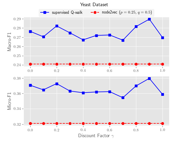
Figure 1: Mean F1 scores of supervised Q-walk against the baseline node2vec for different settings of the discount factor $\gamma$ with fixed $p_{Q}=0.8$, $k_{HN}=1$, $r=24$, $w_{l}=100$, $d=256$, $w_{s}=20$, $e=100$, $v_{l}=0.8$, $\alpha_{0}=1$, $J=100$, $T=3$, $k_{NN}=3$.

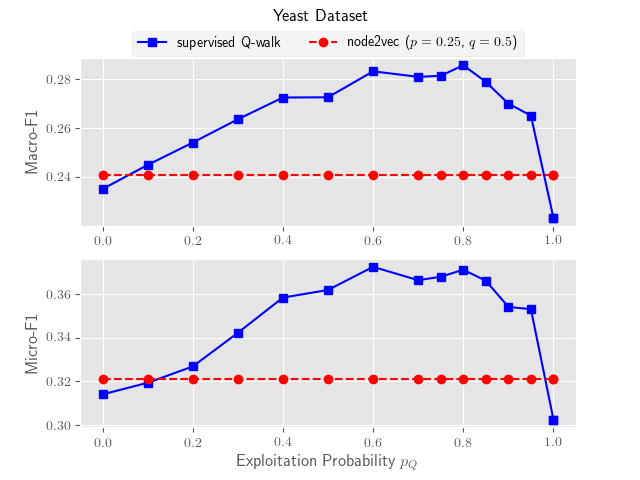
Figure 2: Mean F1 scores of supervised Q-walk against baseline node2vec for different settings of the exploitation probability $p_{Q}$ with fixed $k_{HN}=1$, $r=24$, $w_{l}=100$, $d=256$, $w_{s}=20$, $e=100$, $v_{l}=0.8$, $\alpha_{0}=1$, $J=100$, $T=3$, $k_{NN}=3$, $\gamma=0.9$.

Figure 3: Mean F1 scores of supervised Q-walk against baseline node2vec for different settings of the word2vec epochs $e$ with fixed $k_{HN}=1$, $r=24$, $w_{l}=100$, $d=256$, $w_{s}=20$, $v_{l}=0.8$, $\alpha_{0}=1$, $J=100$, $T=3$, $k_{NN}=3$, $\gamma=0.9$, $p_{Q}=0.8$.

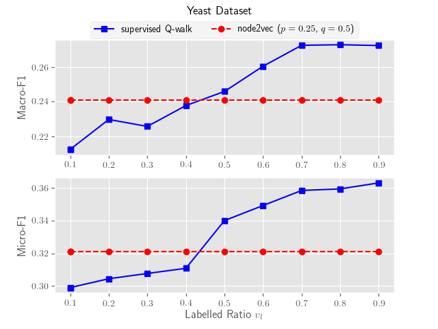
Figure 4: Mean F1 scores of supervised Q-walk against baseline node2vec for different settings of the ratio of labelled nodes $v_{l}$, used for learning confidence values as per III-B with fixed $k_{HN}=1$, $r=24$, $w_{l}=100$, $d=256$, $\alpha_{0}=1$, $J=100$, $T=3$, $k_{NN}=3$, $w_{s}=20,\gamma=0.9$, $p_{Q}=0.8$, $e=100$.

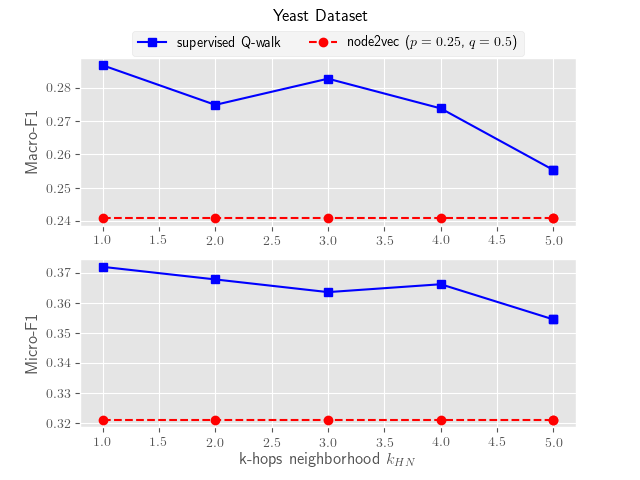
Figure 5: Mean F1 scores of supervised Q-walk against baseline node2vec for different settings of $k_{HN}$, used for learning confidence values as per III-B with fixed $r=24$, $w_{l}=100$, $d=256$, $\alpha_{0}=1$, $J=100$, $T=3$, $k_{NN}=3$, $\gamma=0.9$, $p_{Q}=0.8$, $e=100$, $w_{s}=20,v_{l}=0.8$.

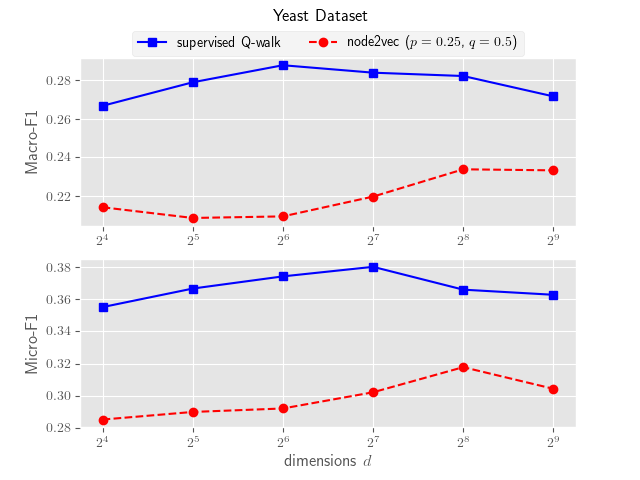
Figure 6: Mean F1 scores of supervised Q-walk against baseline node2vec for different settings of node features representation dimensions $d$ with fixed $r=24$, $w_{l}=100$,$\alpha_{0}=1$, $J=100$, $T=3$, $k_{NN}=3$, $\gamma=0.9$, $p_{Q}=0.8$, $e=100$, $v_{l}=0.8$, $k_{HN}=1,w_{s}=20$.

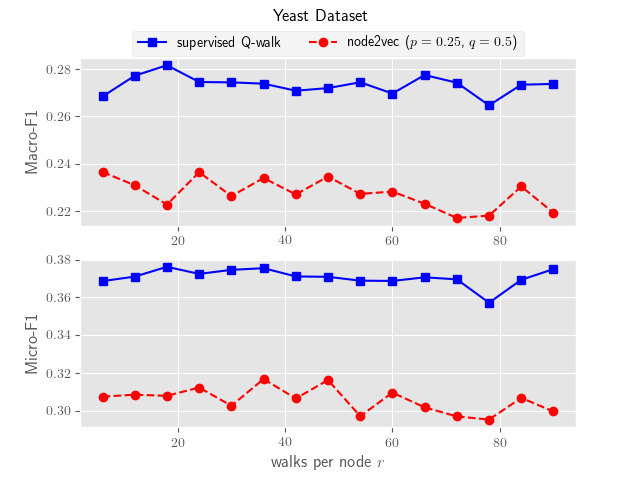
Figure 7: Mean F1 scores of supervised Q-walk against baseline node2vec for different settings of number of walks per node $r$ with fixed $w_{l}=100$,$\alpha_{0}=1$, $J=100$, $T=3$, $k_{NN}=3$, $\gamma=0.9$, $p_{Q}=0.8$, $e=100$, $v_{l}=0.8$, $k_{HN}=1$, $d=256,w_{s}=20$.

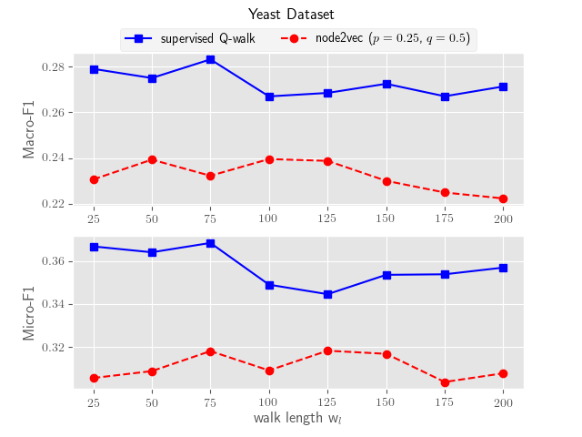
Figure 8: Mean F1 scores of supervised Q-walk against baseline node2vec for different settings of walk length $w_{l}$ with fixed $r=24,\alpha_{0}=1$, $J=100$, $T=3$, $k_{NN}=3$, $\gamma=0.9$, $p_{Q}=0.8$, $e=100$, $v_{l}=0.8$, $k_{HN}=1$, $d=256,w_{s}=20$.

Figure 9: Mean F1 scores of supervised Q-walk against baseline node2vec for different settings of window size $w_{s}$ with fixed $r=24,\alpha_{0}=1$, $J=100$, $T=3$, $k_{NN}=3$, $\gamma=0.9$, $p_{Q}=0.8$, $e=100$, $v_{l}=0.8$, $k_{HN}=1$, $d=256,w_{l}=24$.

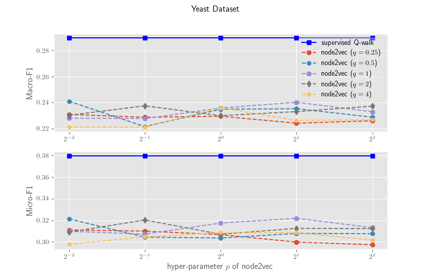
Figure 10: Mean F1 scores of node2vec against supervised Q-walk for different values of $p$ and $q$ with fixed $p_{Q}=0.8$, $k_{HN}=1$, $r=24$, $w_{l}=100$, $d=256$, $w_{s}=20$, $e=100$, $v_{l}=0.8$, $\alpha_{0}=1$, $J=100$, $T=3$, $k_{NN}=3$, $\gamma=0.9,w_{s}=20$.

Table I: Mean F1 scores of supervised Q-walk and node2vec on different datasets with fixed $p_{Q}=0.8$, $k_{HN}=1$, $r=24$, $w_{l}=100$, $d=256$, $w_{s}=20$, $e=100$, $v_{l}=0.8$, $\alpha_{0}=1$, $J=100$, $T=3$, $k_{NN}=3$, $\gamma=0.9$, $p=0.25$, $q=0.5$.

	Supervised Q-walk		node2vec		% improvement
	Macro-F1	Micro-F1	Macro-F1	Micro-F1	Macro-F1	Micro-F1
Yeast	0.2896	0.3797	0.2409	0.3212	20.21%	18.21%
BlogCatalog	0.4051	0.5420	0.1984	0.3062	104.18%	77.01%
Flickr	0.4340	0.5505	0.2087	0.2853	107.95%	92.95%

IV-A Datasets

We provide a brief overview of the datasets which were used to perform the experiments.

IV-A1 Yeast

Yeast [7] dataset is a protein-protein interaction network of budding yeast. It has $2361$ nodes, $7182$ edges and $13$ classes. It is an undirected and unweighted network. It offers a single-label multi-class classification problem.

IV-A2 BlogCatalog

BlogCatalog [25] dataset is a social network of bloggers. The labels associated with the bloggers refer to their interests which are obtained from the metadata information as available on BlogCatalog site. It consists of $10312$ nodes, $333983$ edges and $39$ classes. It is an undirected and unweighted network. It offers a multi-label multi-class classification problem.

IV-A3 Flickr

Flickr [25] dataset is a contact network of users on Flickr site. The labels associated with the users refer to their groups. It consists of $80513$ nodes, $5899882$ edges and $195$ classes. It is an undirected and unweighted network. It offers a multi-label multi-class classification problem.

IV-B Performance Evaluation

We evaluate the performance by first computing the vector representation of nodes in the network using both node2vec and supervised Q-walk for specific hyperparameter settings. Then, we compute the mean of the macro and micro F1 scores obtained by performing 5 fold cross validation using k-nearest neighbors (k-NN) [10] classifier. We use k-NN for a couple of reasons. First, we are interested in showcasing that our learnt embeddings are similar for nodes with same labels, and such similarity can be measured by finding euclidean distance between the node embeddings of the concerned nodes, and this is in accordance with III-A. Second, it is a non-linear classifier, therefore, the learnt embeddings need not be linearly separable for getting better classification performance. We denote $k$ in k-NN as $k_{NN}$.

IV-C Results

It can be observed in 1 that values of $\gamma$ around $0.9$ provide higher performance than other values of $\gamma$ on the Yeast dataset. For $\gamma=0$, the F1 scores are better than a number of other $\gamma$ values which signifies the aptness of the reward function (9), since (13) is then modified to $Q_{j}(u,a)=(1-\alpha_{j})Q_{j-1}(u,a)+\alpha_{j}R(u,a,u^{\prime})$, which does not include $Q_{j-1}(u^{\prime},a^{\prime})$. For $\gamma=0$, on BlogCatalog dataset, supervised Q-walk approach achieves mean Macro-F1 score of $0.4198$ and mean Micro-F1 score of $0.5528$ which are higher than the F1 scores for $\gamma=0.9$ as shown in table I.

In 2, we can observe the tradeoff involved between exploration and exploitation. $p_{Q}=0$ means that we do not make use of the learnt Q-values and have instead resorted to randomly explore the network, thereby, leading to poor performance. $p_{Q}=1$ means that we always make the greedy choice by opting for the action which yields maximum Q-value. This is complete exploitation policy which again leads to poor performance. $p_{Q}=0.8$ rightly balances the tradeoff between exploration and exploitation, thereby, leading to higher F1 scores compared with other values of $p_{Q}$.

In 3, we can observe that supervised Q-walk takes small number of epochs to give high F1 scores. In the case of Yeast dataset, $e=100$ was sufficient. There exists randomness in the curves which can be attributed to different weight initializations in word2vec in different runs of the experiment. The F1 scores stop improving after $e=100$. It signifies that the model is trained and starts overfitting for $e>100$.

In 4, we can observe that supervised Q-walk approach performs better than node2vec given we use around and above 50% labelled nodes for learning the confidence values as per III-B. For lower values of $v_{l}$, the performance is poor because the k-hops neighborhood based confidence values learner did not get enough labelled nodes for properly learning the confidence values. For higher values of $v_{l}$, we can see that the performance improves. In a real world setting, it may not be necessary that we get $v_{l}=0.9$ to train upon, instead, for all other experiments we choose $v_{l}=0.8$ since $80\%-20\%$ split of training and test data is generally used in machine learning.

It can be observed in 5 that $k_{HN}=1$ is sufficient for learning good confidence values, in other words, the confidence values can be determined by just looking at the immediate neighbors of any node $u\in V$.

It can be observed in 6 that $d\in[2^{5},2^{8}]$ give high F1 scores. Supervised Q-walk approach gives better F1 scores than node2vec for different settings of dimensions.

It can be observed in 7 that supervised Q-walk approach gives high F1 scores for $r=18$ while node2vec gives high F1 scores for $r=24$ and low for $r=18$. So, our approach takes lesser number of walks per node to give a better performance than node2vec.

It can be observed in 8 and 9 that supervised Q-walk approach gives better F1 scores than node2vec. Values of $w_{l}$ around $75$ and values of $w_{s}$ around $20$ are good enough for our approach on the Yeast dataset.

It can be observed in 10 that supervised Q-walk approach performs better than node2vec hyperparameterised by different combinations of $p$ and $q$ which control the degree of Depth First Sampling (DFS) and Breadth First Sampling (BFS).

The mean F1 scores are calculated for specific hyperparameter settings which leaves room for improvement by fine tuning the hyperparameters through cross validation with grid search or random search [5] over the hyperparameter space.

IV-D Technologies Deployed

All the experiments were carried out on a server housing 48 core Intel Xeon @ $2.5$ GHz processor, 252 GB RAM with Ubuntu 16.04. The experiments were coded in Python 3.6, using 3rd party libraries - NetworkX [11], Numpy [26], Matplotlib [12], Scikit-learn [21] and Gensim [23].

V Conclusion

We have presented a novel supervised Q-walk approach to generate random walks guided by Q-values and assisted by k-hops neighborhood based confidence values learner. We have shown experimentally that the node embeddings learnt from our approach are similar for the nodes with the same labels. We have also shown that our approach outperforms node2vec in the node classification task.

VI Future Work

Supervised Q-walk works better in the cases where the assumption of homophily in networks holds true. In other networks, nodes which are structurally equivalent may have the same labels e.g. networks of bio-chemical compounds. Our work can be extended by composing another reward function $R(u,a,u^{\prime})=R_{1}(u,a,u^{\prime})+\beta R_{2}(u,a,u^{\prime})$ where $R_{1}$ encourages homophily in networks, $R_{2}$ encourages structural equivalence of nodes and $\beta$ is a hyperparameter which decides the tradeoff between homophily and structural equivalence.

VII Acknowledgements

We acknowledge the valuable insights provided by Dr Robert West, Assistant Professor, Data Science Lab, School of Computer and Communication Sciences, EPFL, Switzerland. His lab had also provided us with the compute infrastructure for carrying out all the experiments.

References

- [1] Amr Ahmed, Nino Shervashidze, Shravan Narayanamurthy, Vanja Josifovski, and Alexander J. Smola. Distributed large-scale natural graph factorization. In Proceedings of the 22Nd International Conference on World Wide Web, WWW ’13, pages 37–48, New York, NY, USA, 2013. ACM.
- [2] Lars Backstrom, Dan Huttenlocher, Jon Kleinberg, and Xiangyang Lan. Group formation in large social networks: Membership, growth, and evolution. In Proceedings of the 12th ACM SIGKDD International Conference on Knowledge Discovery and Data Mining, KDD ’06, pages 44–54, New York, NY, USA, 2006. ACM.
- [3] Mikhail Belkin and Partha Niyogi. Laplacian eigenmaps and spectral techniques for embedding and clustering. In Advances in Neural Information Processing Systems 14, pages 585–591. MIT Press, 2001.
- [4] Richard Bellman. A Markovian Decision Process. Indiana Univ. Math. J., 6:679–684, 1957.
- [5] James Bergstra and Yoshua Bengio. Random search for hyper-parameter optimization. J. Mach. Learn. Res., 13:281–305, February 2012.
- [6] Smriti Bhagat, Graham Cormode, and S. Muthukrishnan. Node classification in social networks. CoRR, abs/1101.3291, 2011.
- [7] D. Bu, Y. Zhao, L. Cai, H. Xue, X. Zhu, H. Lu, J. Zhang, S. Sun, L. Ling, N. Zhang, G. Li, and R. Chen. Topological structure analysis of the protein-protein interaction network in budding yeast. Nucleic Acids Research, 31:2443–2450, 2003.
- [8] Shaosheng Cao, Wei Lu, and Qiongkai Xu. Grarep: Learning graph representations with global structural information. In Proceedings of the 24th ACM International on Conference on Information and Knowledge Management, CIKM ’15, pages 891–900, New York, NY, USA, 2015. ACM.
- [9] Aditya Grover and Jure Leskovec. Node2vec: Scalable feature learning for networks. In Proceedings of the 22nd ACM SIGKDD International Conference on Knowledge Discovery and Data Mining, KDD ’16, pages 855–864, New York, NY, USA, 2016. ACM.
- [10] Gongde Guo, Hui Wang, David Bell, Yaxin Bi, and Kieran Greer. KNN Model-Based Approach in Classification, pages 986–996. Springer Berlin Heidelberg, Berlin, Heidelberg, 2003.
- [11] Aric A. Hagberg, Daniel A. Schult, and Pieter J. Swart. Exploring network structure, dynamics, and function using NetworkX. In Proceedings of the 7th Python in Science Conference (SciPy2008), pages 11–15, Pasadena, CA USA, August 2008.
- [12] J. D. Hunter. Matplotlib: A 2d graphics environment. Computing In Science & Engineering, 9(3):90–95, 2007.
- [13] Jure Leskovec, Daniel Huttenlocher, and Jon Kleinberg. Signed networks in social media. In Proceedings of the SIGCHI Conference on Human Factors in Computing Systems, CHI ’10, pages 1361–1370, New York, NY, USA, 2010. ACM.
- [14] Jure Leskovec, Jon Kleinberg, and Christos Faloutsos. Graph evolution: Densification and shrinking diameters. ACM Trans. Knowl. Discov. Data, 1(1), March 2007.
- [15] Jure Leskovec, Kevin J. Lang, Anirban Dasgupta, and Michael W. Mahoney. Community structure in large networks: Natural cluster sizes and the absence of large well-defined clusters. CoRR, abs/0810.1355, 2008.
- [16] Jure Leskovec and Julian J. Mcauley. Learning to discover social circles in ego networks. In F. Pereira, C. J. C. Burges, L. Bottou, and K. Q. Weinberger, editors, Advances in Neural Information Processing Systems 25, pages 539–547. Curran Associates, Inc., 2012.
- [17] Miller McPherson, Lynn Smith-Lovin, and James M Cook. Birds of a feather: Homophily in social networks. Annual Review of Sociology, 27(1):415–444, 2001.
- [18] Tomas Mikolov, Kai Chen, Greg Corrado, and Jeffrey Dean. Efficient estimation of word representations in vector space. CoRR, abs/1301.3781, 2013.
- [19] Tomas Mikolov, Ilya Sutskever, Kai Chen, Greg S Corrado, and Jeff Dean. Distributed representations of words and phrases and their compositionality. In C. J. C. Burges, L. Bottou, M. Welling, Z. Ghahramani, and K. Q. Weinberger, editors, Advances in Neural Information Processing Systems 26, pages 3111–3119. Curran Associates, Inc., 2013.
- [20] Mingdong Ou, Peng Cui, Jian Pei, Ziwei Zhang, and Wenwu Zhu. Asymmetric transitivity preserving graph embedding. In Proceedings of the 22Nd ACM SIGKDD International Conference on Knowledge Discovery and Data Mining, KDD ’16, pages 1105–1114, New York, NY, USA, 2016. ACM.
- [21] F. Pedregosa, G. Varoquaux, A. Gramfort, V. Michel, B. Thirion, O. Grisel, M. Blondel, P. Prettenhofer, R. Weiss, V. Dubourg, J. Vanderplas, A. Passos, D. Cournapeau, M. Brucher, M. Perrot, and E. Duchesnay. Scikit-learn: Machine learning in Python. Journal of Machine Learning Research, 12:2825–2830, 2011.
- [22] Bryan Perozzi, Rami Al-Rfou, and Steven Skiena. Deepwalk: Online learning of social representations. In Proceedings of the 20th ACM SIGKDD International Conference on Knowledge Discovery and Data Mining, KDD ’14, pages 701–710, New York, NY, USA, 2014. ACM.
- [23] Radim Řehůřek and Petr Sojka. Software Framework for Topic Modelling with Large Corpora. In Proceedings of the LREC 2010 Workshop on New Challenges for NLP Frameworks, pages 45–50, Valletta, Malta, May 2010. ELRA. http://is.muni.cz/publication/884893/en.
- [24] Sam T. Roweis and Lawrence K. Saul. Nonlinear dimensionality reduction by locally linear embedding. SCIENCE, 290:2323–2326, 2000.
- [25] Lei Tang and Huan Liu. Relational learning via latent social dimensions. In Proceedings of the 15th ACM SIGKDD International Conference on Knowledge Discovery and Data Mining, KDD ’09, pages 817–826, New York, NY, USA, 2009. ACM.
- [26] Stefan van der Walt, S. Chris Colbert, and Gael Varoquaux. The numpy array: A structure for efficient numerical computation. Computing in Science and Engg., 13(2):22–30, March 2011.
- [27] Christopher J.C.H. Watkins and Peter Dayan. Technical note: Q-learning. Machine Learning, 8(3):279–292, 1992.