From the bulk electrolyte solution to the electrochemical interface

Abstract

This paper is aiming at presenting some relevant contributions of Jean-Pierre Badiali during the first ten years of his growing scientific activity. This presentation does not contain new materials but is based on a number of selected papers published in the seventies, a part of them written in French. The presentation is organized around three points. The first point, corresponding to his PhD thesis, is concerned with the study of ion-solvent and ion-ion interactions in a solution using complex dielectric permittivity measurements in the Hertzian and microwave frequency range. The second one is concerned with an analysis of the ion pair absorption band observed in the far infrared region in terms of an interionic potential energy. The third one is concerned with the metal-solution interface and his significant advances on (i) the Lippmann equation linking electrocapillary and electrical measurements and (ii) the contribution of the metal to the differential interfacial capacity.

Key words: dielectric spectroscopy, ionic conductivity, surface tension, interfacial capacitance

PACS: 71-10.Ay, 73-20.At, 77-22, 78-30.cd, 82-45.Fk

Abstract

Метою статтi є представлення важливого внеску Жана-П’єра Бадiалi впродовж перших десяти рокiв його стрiмкої наукової дiяльностi. Вона не мiстить нового матерiалу, проте базується на низцi вибраних статтей, опублiкованих в 70-х роках, частина з яких написана французькою мовою. Стаття представляє три аспекти. Перший, що вiдповiдає тематицi дисертацiї доктора фiлософiї, присвячений вивченню взаємодiй ‘‘iон-розчинник’’ та ‘‘iон-iон’’ в розчинi з використанням складних вимiрювань дiелектричної проникностi в дiапазонi Герцiв i мiкрохвильових частот. Другий аспект стосується аналiзу зони поглинання iонних пар, яка спостерiгається в далекiй iнфрачервонiй областi в термiнах мiжiонної потенцiальної енергiї. Третiй пов’язаний з поверхнею роздiлу ‘‘метал-розчин’’, i важливими досягненнями тут є: (i) рiвняння Лiппмана, яке пов’язує електрокапiлярнi та електричнi вимiрювання; (ii) внесок металу в диференцiальну iнтерфейсну електричну ємнiсть.

Ключовi слова: дiелектрична спектроскопiя, iонна провiднiсть, поверхневий натяг, iнтерфейсна ємнiсть

1 Introduction

This paper is written in memory of Jean-Pierre Badiali, providing a survey of his contribution during the first ten years of his scientific activity. As a matter of fact, this paper does not contain new results. It is based on the bibliography of J.P. Badiali as given in the references. Initially, he had a general training in electrical engineering without a particular predisposition in the field of electrochemistry. In 1967, he entered the C.N.R.S. research group n°4 “Physics of Liquids and Electrochemistry”, directed by Prof. I. Epelboin. More specifically, he joined the team led by Dr. J.C. Lestrade, with the main objective to investigate the dielectric properties of electrolyte solutions, considered as partners of the electrochemical interfaces. In the sixties and seventies, a large number of laboratories around the world were invested in applying dielectric spectroscopy for studying molecular motions in pure liquids, which means measuring the complex dielectric permittivity in a large frequency domain including microwaves. In the case of electrolyte solutions, the number of laboratories involved was much less, notably in UK the pioneer group led by J.B. Hasted [1] and in Germany those of R. Pottel [2] and J. Barthel [3]. A reason for that was the experimental difficulty arising from the electrical conductivity of ionic solutions. Thus, measurements below c.a. 100 MHz are dominated by the losses due to the ionic conductivity preventing from reaching the so-called static dielectric constant of the medium, contrary to the case of pure liquids. Another limiting factor at this time was the necessity to develop several experimental set-ups (often one per frequency) to cover all the required frequency range. When preparing his PhD thesis [4], his first task was to complete the existing experimental set-ups covering the frequency range, 0.1 to 10 GHz, by building a waveguide interferometer functioning at 35 GHz. As it will be shown later, this extended frequency domain was very useful to analyze the relaxation processes arising from molecular and ionic motions, at the source of his first theoretical derivations. The present paper is divided into three parts, corresponding to three relevant contributions of J.P. Badiali. The first one will be devoted to the modeling of ionic relaxation process, as evidenced from spectroscopic measurements in organic solvents with a low dielectric constant [5, 6, 7, 8, 9, 10]. The second one concerns the emerging THz spectroscopy applied to highly absorbing liquids [11, 12], with the observation of an absorption band in the far infrared region (20 to 150 cm^-1) related to the vibration of a cation-anion pair and the interpretation of the frequency corresponding to the absorption maximum in terms of an interionic potential [13, 14, 15]. The third one will refer to the electrochemical interface, from the point of view of surface tension and differential capacitance [16, 17, 18, 19, 20]. This was in the context of developing microscopic physical models of the metal-ionic solution interface using a statistical mechanical treatment of the whole interface [21, 22].

2 Dielectric spectroscopy of electrolyte solutions

2.1 Generalities

As mentioned in the introduction, dielectric spectroscopy is based on the measurements of the complex dielectric permittivity $\varepsilon^{*}=\varepsilon^{\prime}-\mathrm{i}\varepsilon^{\prime\prime}$ with ($\mathrm{i}^{2}=-1$) in a frequency range sufficiently wide to get a reliable information both on the static properties of the medium (the so-called dielectric constant) and on different relaxation processes arising from molecular and ionic motions. It is worthwhile recalling that the dielectric permittivity expresses the response in terms of current density of a medium submitted to a perturbation of electric field. In the case of pure polar liquids, in the Hertzian frequency range (a few dozens of MHz to a few dozens of GHz), the observed response is that of rotation of molecular species. When considering electrolyte solutions, motion of charge carriers, as translational displacements, should now be taken into account. On the basis of statistical mechanics considerations, using the formalism of microscopic Maxwell equations, a general expression for the complex dielectric permittivity $\varepsilon^{*}(\omega)$ of an electrolyte solution was established as:

$$\varepsilon^{*}(\omega)=\varepsilon^{*}_{\text{d}}(\omega)+\frac{\sigma_{0}}{\mathrm{i}\omega\varepsilon_{0}}+H^{*}(\omega),$$ (2.1)

where $\sigma_{0}$ is the low frequency conductivity, $\omega$ is the angular frequency and $\varepsilon_{0}=8.84\cdot 10^{-12}$ F/m [7, 8, 9]. Conductivity losses, expressed as $\sigma_{0}/(\mathrm{i}\omega\varepsilon_{0})$, become a dominating contribution to $\varepsilon$ at low frequencies. The first term $\varepsilon_{\text{d}}^{*}(\omega)$ represents the response of molecular species. The third term $H^{*}(\omega)$ represents the frequency dependent contribution of ions, including cross effects between ions and molecular dipoles.

2.2 Solution spectrum analogous to solvent spectrum

This case corresponds to a charge transport independent of frequency, which means only represented by a static conductivity $\sigma_{0}$, the one which can be measured at audio frequencies. In this way, the overall complex dielectric permittivity reads: $\varepsilon^{*}=\varepsilon_{\text{d}}^{\prime}+\mathrm{i}[\varepsilon^{\prime\prime}_{\text{d}}+\sigma_{0}/(\mathrm{i}\omega\varepsilon_{0})]$, where $\varepsilon_{\text{d}}^{\prime}$ and $\varepsilon^{\prime\prime}_{\text{d}}$ only refer to the solvent relaxation process. Such a situation is usually encountered for solutions with solvents having a high dielectric constant, for instance water, methanol, ethanol, N,N-dimethylformamide (DMF) [5, 6]. Any change in the solvent relaxation parameters can be attributed to the short range ion-solvent interactions. In a general way, it has been established that the observed decrease of the solvent static permittivity $\varepsilon_{\text{s}}(c)$, when increasing the salt concentration $c$, provided a quantitative information on the ion solvation process. In agreement with experiments, at low salt concentrations, $\varepsilon_{\text{s}}(c)$ is a linear relation, with a slope $\delta$. The static solvent permittivity $\varepsilon_{\text{s}}$ is conveniently described by the Kirkwood-Fröhlich expression:

$$\varepsilon_{\text{s}}-\varepsilon_{\infty}=\frac{3\varepsilon_{\text{s}}}{2\varepsilon_{\text{s}}+\varepsilon_{\infty}}\frac{N}{3kT\varepsilon_{0}}\left(\frac{\varepsilon_{\infty}+2}{3}\right)^{2}{g\mu^{2}},$$ (2.2)

in which $\varepsilon_{\infty}$ represents the electronic and atomic contribution to the permittivity, $\mu$ is the dipole moment of a solvent molecule in vacuum, $k$ is the Boltzmann constant, $T$ is the absolute temperature, $N$ is the number of solvent molecules per volume unit participating in the polarization of orientation and $g$ is the correlation factor between neighboring solvent dipoles. Using the above formula, a linear relation for $\varepsilon_{\text{s}}(c)$ yields a linear relation for $N(c)$ as $N(c)=N_{0}-qc$ with the following expression for $q$:

$$q=\frac{N_{{0}}\delta}{\varepsilon_{\text{s}0}}\frac{2\varepsilon_{\text{s}0}^{2}+\varepsilon_{\infty}^{2}}{\left(\varepsilon_{\text{s}0}-\varepsilon_{\infty}\right)\left(2\varepsilon_{\text{s}0}+\varepsilon_{\infty}\right)}\,.$$ (2.3)

As a result, $q$ is an estimate of a solvation number defined as the number of rotation-blocked solvent molecules per molecule of salt. It has been shown that for cations such as Li⁺, Na⁺, Mg²⁺, the short range cation solvent molecule interactions could be coordinated bonds formation at the number of 4 per cation, in a tetrahedral configuration. For symmetry reason, the solvated cations bear no permanent dipole moment. Anions such as ClO${}_{4}^{-}$ are assumed to be not solvated and small anions such as halides may interact with molecules but without building well defined non-polar structures. A number of significant data are given in table 1, showing that the number of blocked molecules are found to be very high in hydrogen bonded solvents due to their self-association. In alcohols, the solvation shell is not limited to the molecules coordinated with the cation but involves rigid molecular chains, the mean number of molecules per chain being given by the quantity $f$. For a simple liquid such as DMF without dipolar correlations, $f$ is close to 1, the number of blocked molecules is close to 4, as predicted by the cation solvation model.

Table 1: Effect of solvent intermolecular structure on the short range ion-solvent interactions as measured by the solvation number $q$.

	Self-associated protic solvents						3cmNon-associated
aprotic solvent
solvent	Ethanol			Methanol			DMF
Salt	LiClO4	Mg(ClO4)2	LiCl	LiCLO4	NaClO4	Mg(ClO4)2	NaClO4
$\delta$, mol${}^{-1}\cdot$ L	25.4 $\pm$ 9.6	20.7 $\pm$ 6.6	26.6 $\pm$ 2.5	38.6 $\pm$ 3.9	31.5 $\pm$ 5.3	32.7 $\pm$ 5.9	14.4 $\pm$ 2.6
$q$	18.5 $\pm$ 7	15.1 $\pm$ 4.8	19.5 $\pm$ 1.8	30 $\pm$ 3.1	27 $\pm$ 4.2	25.8 $\pm$ 4.7	4.6 $\pm$ 0.9
$f$	5 $\pm$ 1			7 $\pm$ 1			$\approx 1$

2.3 Solution spectrum with additional ionic relaxation process

Dielectric experiments of ionic solutions in weakly polar solvents, such as acetone, ethyl acetate, tetrahydrofuran (THF), clearly evidence a new relaxation process in addition to that of the solvent [7, 10]. A first attempt in literature to interpret this phenomenon was to consider the ion pair formation, in a way analogous to what was done in classical theories of conductivity of dilute electrolytes. Ion pairing is based on the static concept of a chemical equilibrium between ion pairs and free ionic species. Neutral ion pairs do not participate in charge transport and are capable of rotating as molecular dipoles with a definite dipole moment. Such an approach gives rise to several objections: (i) at relatively high salt concentrations, necessary to extract the ionic contribution from dielectric experiments, ionic aggregates of the orders higher than ion pairs should be introduced, as done in conductivity theories; (ii) ion pair cannot be actually considered as having an infinite life-time. To clarify these objections, Badiali et al. derive a formal theoretical expression for the conductivity and its frequency dependence which will be briefly summarized below [7]. It has been shown that the time dependence of the current density $I(t)$ could be written as:

$$I(t)=\frac{1}{3kTV}\int_{0}^{t}\langle\dot{M}(0)\dot{M}(\tau)\rangle E(t-\tau)\mathrm{d}\tau.$$ (2.4)

In equation (2.4), $\dot{M}$ is the time derivative of the electrical moment $M$ of all the entities inside the volume $V$, the neutral ones (solvent molecules) with moment $M_{\text{m}}$, the charged species (ions, solvated or not, other charged aggregates) with moment $M_{\text{c}}$, with $M=M_{\text{m}}+P_{\text{c}}$. This decomposition of $M$ when inserted into equation (2.4) gives rise to three time dependent current contributions, (i) molecular relaxation; (ii) ionic relaxation leading to a frequency dependent conductivity $\sigma(\omega)$; (iii) coupling between dipolar and charged species usually considered as negligible. The following expression was derived for the frequency dependent conductivity $\sigma(\omega)$:

$$\sigma(\omega)=\sigma(0)+\mathrm{i}\omega\frac{1}{3kTV}\langle M_{\text{c}}^{2}(0)\rangle\left[1-\mathrm{i}\omega\int^{\infty}_{0}\mathrm{e}^{-\mathrm{i}\omega\tau}\frac{\langle M_{\text{c}}(0)M_{\text{c}}(\tau)\rangle}{M_{\text{c}}^{2}(0)}\mathit{\mathrm{d}\tau}\right].$$ (2.5)

Then, the spectral response of electrolytes is connected with the self-correlation function of the electrical moment of all the ions in a given volume. Using the above expression, a statistical model of charge transport was derived considering around an anion the relative motion of a cation perturbed by collisions with other species with a probability $p$ to be weak, $(1-p)$ to be strong, and a linear motion between collisions. The collision times are assumed to be distributed according to a Poisson process. It leads to a class of non-exponential correlation functions as suggested by experiments. In the special case of a linear Brownian motion between collisions, an analytical expression was obtained for the ionic conductivity $\sigma(\omega)$. It can be expressed in terms of a complex permittivity $\varepsilon_{\text{c}}(\omega)$:

$$\varepsilon_{\text{c}}(\omega)=\frac{\sigma(\omega)}{\mathrm{i}\omega\varepsilon_{0}}=\frac{\sigma(0)}{\mathrm{i}\omega\varepsilon_{0}}+\frac{\Delta\varepsilon}{1+\mathrm{i}\omega\tau}\left(1+\gamma\frac{\mathrm{i}\omega\tau}{\sqrt{1+a+\mathrm{i}\omega\tau}}\right).$$ (2.6)

The second term in equation (2.6) provides an analytical expression to the $H^{*}(\omega)$ function appearing in the general expression of the response $\varepsilon^{*}(\omega)$ of an electrolyte solution (2.1). This model was successful for representing the experimental data of electrolyte solutions in weakly polar solvents. As an example, figure 1 shows the variations of the real and imaginary parts of $\varepsilon^{*}(\omega)$ with frequency in the case of solutions of LiClO₄ in tetrahydrofuran at 30°C. The agreement between model and experiments is of the order of 1% on the real and imaginary parts of $\varepsilon^{*}(\omega)$.

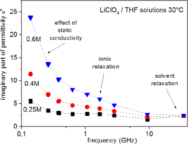
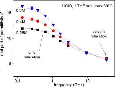
Figure 1: (Color online) Variations with frequency of the real and imaginary parts of $\varepsilon^{*}(\omega)$ for LiClO₄/tetrahydrofuran solutions at 30^∘C: ($\blacksquare$) 0.25M; ($\bullet$) 0.4M; ($\blacktriangledown$) 0.6M. The lines correspond to the numerical fit of the frequency dependent conductivity model completed by the contribution of solvent relaxation of the Debye type (relaxation time: $\tau_{\text{d}}$ = 2.3 ps; dielectric constant: 7.22 at 30^∘C).

Table 2: Parameters extracted from the numerical analysis of the permittivity data of LiClO₄/THF solutions according to the full expression given at the top of the table; $\varepsilon_{\infty}$ ($=2.19$) and $\tau_{\text{d}}$ ($=2.3$ ps) were fixed at their values for the pure solvent.

$\displaystyle\varepsilon_{\text{c}}(\omega)=\frac{\sigma(0)}{\mathrm{i}\omega\varepsilon_{0}}+\frac{\Delta\varepsilon}{1+\mathrm{i}\omega\tau}\left(1+\gamma\frac{\mathrm{i}\varpi\tau}{\sqrt{1+a+\mathrm{i}\omega\tau}}\right)+\frac{\varepsilon_{\text{s}}-\varepsilon_{\infty}}{1+\mathrm{i}\omega\tau_{\text{d}}}+\varepsilon_{\infty}$
Salt molar	$\varepsilon_{\text{s}}$	$\Delta\varepsilon$	$\sqrt{\langle R^{2}(0)\rangle}$, nm	$\tau$, ps	$p=a/(1+a)$	$\sigma_{0}$, S/m	Fit quality
concentration
0.25	6.72	5.3	0.38	126	0.32	0.039	1.04
0.4	6.14	7.9	0.37	194	0.43	0.081	0.91
0.6	5.97	10.2	0.34	136	0.65	0.171	1.04

Table 2 shows the full expression of $\varepsilon^{*}(\omega)$ used to represent the experimental spectra and the values of the relevant parameters obtained by numerical fitting. As previously, the static dielectric constant of the solvent $\varepsilon_{\text{s}}$ decreases at an increasing salt concentration, in agreement with a solvation number close to 4. The characteristic time of relaxation of ionic atmosphere $\tau$ lies in the range 130–200 ps, one hundred times larger than the dipole rotation time. The probability factor $p$ for the occurrence of weak collisions turns around 0.5. The mean anion-cation quadratic distance $\delta_{\text{ac}}=\sqrt{\langle R^{2}(0)\rangle}$ can be calculated from the amplitude $\Delta\varepsilon$ of the ionic relaxation according to:

$$\sqrt{\langle R^{{2}}(0)\rangle}=\frac{3kT\varepsilon_{0}}{e^{2}}\frac{\Delta\varepsilon}{N/V}\,,$$ (2.7)

where $e$ is the electronic charge. The values of $\delta_{\text{ac}}$ are slightly higher than the sum of the crystallographic radii (0.26 nm), in good agreement with the fact that the cation is solvated and that the ion pair is a fluctuating labile structure.

3 Interionic potential energy and far-infrared signature

As mentioned above, the microwave properties of electrolyte solutions in non-aqueous solvents consist mainly in an excess dielectric polarization and absorption which is interpreted in terms of ionic processes at the time scale of about $10^{-9}$ s. A realistic interpretation of this phenomenon was proposed, based on a stochastic description of the translational diffusion of ions, perturbed by instantaneous collisions. In the far-infrared range (FIR), at millimeter and submillimeter wavelengths (10 to 150 cm^-1 wave numbers), molecular liquids present an absorption originating from rotational motion, combined eventually with low frequency vibration modes. In the presence of ions, additional effects can occur due to ion-ion and ion-solvent interactions, each one depending on the nature of the solvent and ions. In what follows, we are dealing with the FIR response of tetraalkylammonium halides R₄NX for which a model for the ion-ion pair potential energy was elaborated. FIR spectra of R₄NX in solvents such as benzene, carbon tetrachloride and chloroform are characterized by a very broad and asymmetric absorption band, the frequency position $\nu_{\text{L}}$ being anion dependent, as depicted in figure 2 [13, 14, 15].

This is in agreement with the harmonic oscillator model for the anion-cation pair, the resonant frequency $\nu_{\text{L}}$ being related to the force constant $k_{\text{L}}$:

$$\nu_{\text{L}}=\frac{1}{2\piup c_{0}}\sqrt{\frac{k_{\text{L}}}{m_{+-}}}\,,$$ (3.1)

where $c_{0}$ is the light velocity and $m_{+-}$ is the reduced mass of the ion pair, close to the anion mass because the cation is much heavier than the anion. It was shown that a realistic effective pair potential $u_{ij}$ could be derived from properties of the salt in the solid state. The proposed form was:

$$u_{ij}(r_{ij})=\frac{1}{4\piup\varepsilon_{0}}\left[\frac{e_{i}e_{j}}{r_{ij}}-\frac{(\alpha_{i}+\alpha_{j})e^{2}}{2r_{ij}^{4}}-\frac{c_{ij}e^{2}}{r_{ij}^{6}}+\frac{be^{2}}{r_{ij}^{9}}\right],$$ (3.2)

where $r_{ij}$ is the distance between the ions $i$ and $j$, having a charge $e_{i}$ or $e_{j}$, and polarizabilities $\alpha_{i}$ or $\alpha_{j}$, respectively. If $r_{\text{L}}$ is the equilibrium distance between the centers of both charges, the force constant $k_{\text{L}}$ governing the band position is given by:

$$k_{\text{L}}=\frac{e^{2}}{4\piup\varepsilon_{0}}\left(\frac{90b}{r_{\text{L}}^{11}}-\frac{2}{r_{\text{L}}^{3}}-\frac{20\alpha}{r_{\text{L}}^{6}}-\frac{42c}{r_{\text{L}}^{8}}\right).$$ (3.3)

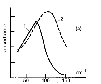
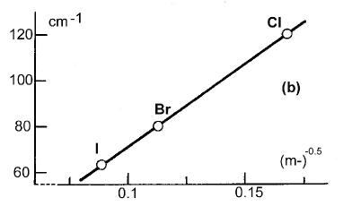
Figure 2: FIR behavior of tetra-alkylammonium halides: (a) absorption spectra of Pr₄NBr in chloroform (1); Bu₄NCl in a 5% v/v acetone/CCl₄; (b) dependence of the maximum absorption frequency on the anion mass $m_{-}$.

In this expression, $b$ is determined from the properties of the solid. Assuming a body-centered cubic arrangement (CsCl type) for the structure of R₄NX when unknown leads to calculated frequencies in satisfying agreement for the solid salts but lower than the experimental ones in solution. A more refined calculation was done in the case of tetrapropylammonium bromide Pr₄NBr for which the actual structure is known as a zinc sulfide type arrangement. Due to a tetragonal structure, there is a distribution of frequencies according to the crystallographic directions. As shown in table 3, the $b$ parameter relative to the repulsive term is strongly dependent on the structure, and the right structure leads to a fine agreement between experimental and calculated $\nu_{\text{L}}$ frequencies, validating the physical image of an ion pair vibrator in solution at the $10^{-12}$–$10^{-13}$ s time scale.

Table 3: Calculated and experimental frequencies $\nu_{\text{S}}$ (solid) and $\nu_{\text{L}}$ (in solution) for Pr₄NBr.

Pr4NBr
Structure	$10^{76}\cdot b$, m8	$\nu_{\text{S}}$, cm-1	$\nu_{\text{L}}$, cm-1
Cubic	25.5	56	55
Tetragonal	7.2	85 to 98	78
Experimental values		48-71-104	80

4 Electrochemical interface

Among the possible electrochemical systems, the ideally polarisable electrochemical interface is the simplest one, in the sense that no charge transfer occurs across it. The most widely studied example is given by the mercury drop electrode, which allows one to perform electrocapillary and electrical impedance measurements. Such an ideal system was an attractive field for Badiali to develop a general statistical mechanical treatment in comparison with the usual thermodynamic approach. The first important contribution was concerned with the notion of surface tension, more precisely with the Lippmann equation, the second one was concerned with the contribution of the metal to the differential capacitance of the ideally polarized electrode.

4.1 The Lippmann equation

The Lippmann equation is concerned with the surface tension $\gamma$ of the interface between an ideally polarisable electrode and an ionic solution. According to this equation, the change in surface tension $\Delta\gamma$, divided by the change in the potential drop across the interface $\Delta U$, gives the negative of the surface charge density $Q$. As a consequence, the second derivative of the surface tension with potential can be identified with the capacity of the double layer $C_{\text{dl}}$ obtained from impedance measurements. It reads:

$$\Delta\gamma/\Delta U=-Q\qquad\mbox{and}\qquad-\partial^{2}\gamma/\partial^{2}U=C_{\text{dl}}\,.$$ (4.1)

When derived by thermodynamics, the quantities appearing in the Lippmann equation do not refer to the actual charge distribution in the interfacial region. The original work of Badiali and Goodisman was to derive the Lippmann equation by statistical mechanical methods on the basis of a model at the molecular level, enabling all the quantities appearing in the model to have a physical definition [16, 17]. The first step was to derive the conditions for mechanical equilibrium in the presence of an electric field of a system with inhomogeneous and anisotropic properties. From the balance of forces, equations were obtained for the surface tension in terms of the pressure, electric field, electric charge density, and electric polarization at each point within the system. Having in mind the mercury drop electrode, a spherically symmetric system was considered, allowing a direct calculation of the change in the surface tension $\Delta\gamma$ produced by a change in the potential drop $\Delta U$, maintaining thermal equilibrium, constant temperature, and the pressure and chemical composition in homogeneous regions. A surface on which the charge density is always zero was introduced within the interface, allowing the surface charge to be defined as the integral of the charge density over the metal side of the interface. Only the solution side was treated by statistical mechanics using Boltzmann distributions for charged and polarisable species. The Lippmann equation was successfully derived in two cases: (i) considering only ions and assuming a dielectric constant equal to that of vacuum; (ii) considering ions and molecules in thermal equilibrium, and a dielectric constant varying from a point to point and changing with the field. It was emphasized that, in a coherent model, it was inadmissible of reducing the solvent to a medium of fixed dielectric constant. Finally, considering the response of the system to an imposed alternating potential, within the low frequency limit, it was demonstrated that the system behaves as a pure capacitance with a value equal to the derivative of the above mentioned surface charge density with respect to the potential drop across the interface.

4.2 Contribution of the metal to the interfacial differential capacity

Experimentally, it was found that the point of zero charge (pzc) and the interfacial differential capacity of a metal-solution interface are dependent on the metal. To understand this dependence, Badiali et al. firstly intended to calculate how the surface potential can be modified by the metal solvent interaction at the pzc [18], and subsequently with the charge on the metal in view of calculating the interfacial capacitance [19, 20]. The model for the metal surface in contact with a solvent they retained was the so-called ‘‘dielectric field model’’ represented in figure 3 with parameters for an aqueous solution. Assuming no specific adsorption, the metal should be in contact with a monolayer of water, whose thickness $d_{2}-d_{1}$ is about 0.3 nm and attributing a relative dielectric permittivity $\varepsilon_{1}=6$ for the fixed dipoles. It is assumed that the water monolayer is bounded by an ideal charged plane (located at $d_{2}$), beyond which one has an unperturbed solvent with dielectric permittivity $\varepsilon_{1}=78$. The distance $d_{1}$ is the distance of the closest approach between the metal ion cores and the center of adsorbed solvent molecules. A calculation of $d_{1}$ was proposed by Kornyshev and Vorotyntsev, about 0.13 nm in the case of mercury [23]. For Badiali et al., $d_{1}$ was considered as an equilibrium distance as the result of metal-solution coupling, which is charge dependent.

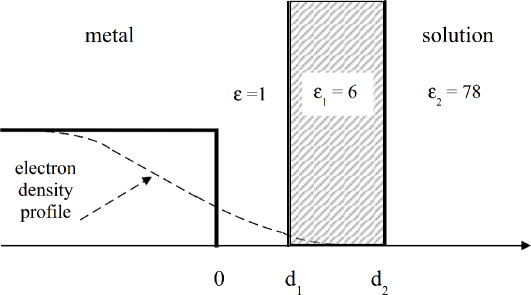
Figure 3: Dielectric field model used to discuss the interaction of solvent molecules with metal electrons.

Using a two-parameter exponential profile for electrons, the above model leads to an expression of the interfacial differential capacity $C$ at the pzc:

$$\frac{1}{C}=\frac{d_{2}-d_{1}}{\varepsilon_{0}\varepsilon_{1}}+\frac{d_{1}}{\varepsilon_{0}}+\frac{1}{C^{\text{M}}(\text{dip})}\,.$$ (4.2)

$C^{\text{M}}(\text{dip})$ corresponds to the relaxation of the electronic structure with the charge on the metal. This approach has successfully taken into account the large difference in the capacitance values obtained for a mercury electrode $C(\text{Hg})=28$ F/cm², and for a gallium electrode $C(\text{Ga})=135$ F/cm², emphasizing the crucial role played by the metal in determining the value of the interfacial capacity.

5 Conclusion and perspectives

The research works presented in this paper reflect a certain state of the art forty or fifty years ago. A number of progresses have been made since that time. This is particularly the case for the ultra-broadband dielectric spectroscopy (1 MHz to 10 THz), mainly due to technological developments, although several different apparatuses with limited bandwidth remain still required for covering the full frequency range. For instance, by the use of network analyzers it becomes possible to record a dielectric spectrum over three decades within a minute instead of hours [24]. The advantages and capabilities of modern dielectric spectroscopy for investigating ion-ion and ion-solvent interactions can be found in the review paper of Buchner and Hefter [25]. For the electrochemical interface, the 1980s were a very fruitful period through the development of truly molecular models for the whole interphase based on jellium for the metal and on ensembles of hard spheres for the electrolyte solution. Such a mathematical description of the metal-solution interface, in which Badiali was an active contributor, was progressively completed by numerical experiments of increasing complexity as stated in [26]. As an example, such theoretical experiments were performed to describe the branching pattern of the capacitance-voltage curves at the metal — ionic solution interface [27]. The tendency in recent works is the shift from aqueous systems to ionic liquids to understand the bell or camel-shaped capacitance-potential curve around the point of zero charge, not explainable within the classical Gouy, Chapman and Stern theory [28].

From the above review, it is clear that J.P. Badiali was early on interested in providing a physical explanation of a number of experimental facts in the field of electrochemistry, using fundamental theoretical approaches. This attitude was always his during his brilliant career of researcher.

Ukrainian 0

Вiд об’ємного розчину електролiту до електрохiмiчного iнтерфейсу Г. Каше${}^{\textsf{\footnotesize{\mbox{?},\penalty 1000\mbox{?}}}}$

             
${}^{\textsf{\footnotesize 1}}$ Нацiональний центр наукових дослiджень Францiї, Лабораторiя iнтерфейсiв та електрохiмiчних систем, Париж, Францiя ${}^{\textsf{\footnotesize 2}}$ Унiверситет Сорбонна, Унiверситет iменi П’єра та Марiї Кюрi, Унiверситет м. Париж, Париж, Францiя

References

- [1] Hasted J.B., Roderick G.W., J. Chem. Phys., 1958, 29, 17, doi:10.1063/1.1744418.
- [2] Pottel R., Ber. Bunsen Ges. Phys. Chem., 1965, 69, 363, doi:10.1002/bbpc.19650690502.
- [3] Barthel J., Schmithals F., Behret H., Z. Phys. Chem., 1970, 71, 115, doi:10.1524/zpch.1970.71.1_3.115.
- [4] Badiali J.P., Contribution à l’Étude des Processus de Relaxation Électrique dans les Solutions Électrolytiques. Relation avec la Solvatation et l’Association Ionique, Ph.D. thesis, Paris, 14th April 1969.
- [5] Badiali J.P., Cachet H., Govaerts F., Lestrade J.C., C.R. Acad. Sci., 1967, 265, 149.
- [6] Badiali J.P., Cachet H., Lestrade J.C., J. Chim. Phys., 1967, 64, 1350, doi:10.1051/jcp/1967641350.
- [7] Badiali J.P., Cachet H., Lestrade J.C., Ber. Bunsen Ges. Phys. Chem., 1971, 75, 297.
- [8] Badiali J.P., Lestrade J.C., J. Chim. Phys., 1969, 66, 107, doi:10.1051/jcp/196966s20107.
- [9] Badiali J.P., Lestrade J.C., J. Chim. Phys., 1970, 67, 667, doi:10.1051/jcp/1970670667.
- [10] Badiali J.P., Cachet H., Lestrade J.C., Electrochim. Acta, 1971, 16, 731, doi:10.1016/0013-4686(71)85041-7.
- [11] Barker C., Yarwood J., J. Chem. Soc., Faraday Trans. 2, 1975, 71, 1322, doi:10.1039/F29757101322.
-
[12]
Bennouna M., Cachet H., Lestrade J.C., Birch J., Chem. Phys., 1981, 62, 439,
doi:10.1016/0301-0104(81)85137-3. - [13] Aimoné L., Badiali J.P., Cachet H., J. Chem. Soc., Faraday Trans. 2, 1977, 73, 1607, doi:10.1039/f29777301607.
- [14] Aimoné L., Badiali J.P., Cachet H., Lestrade J.C., In: Protons and Ions Involved in Fast Dynamic Phenomena, Laszlo P. (Ed.), Elsevier Scientific Publishing Company, Amsterdam, New York, 1978.
- [15] Badiali J.P., Cachet H., Lestrade J.C., Pure Appl. Chem., 1981, 53, 1383.
-
[16]
Badiali J.P., Goodisman J., J. Electroanal. Chem. Interfacial Electrochem., 1978, 91, 151,
doi:10.1016/S0022-0728(78)80097-7. - [17] Badiali J.P., Goodisman J., J. Phys. Chem., 1975, 79, 223, doi:10.1021/j100570a007.
-
[18]
Badiali J.P., Rosinberg M.L., Goodisman J., J. Electroanal. Chem. Interfacial Electrochem., 1981, 130, 31,
doi:10.1016/S0022-0728(81)80374-9. -
[19]
Badiali J.P., Rosinberg M., Goodisman J., J. Electroanal. Chem. Interfacial Electrochem., 1983, 143, 73,
doi:10.1016/S0022-0728(83)80255-1. - [20] Badiali J.P., Electrochim. Acta, 1986, 31, 149, doi:10.1016/0013-4686(86)87100-6.
-
[21]
Badiali J., Rosinberg M.L., Vericat F., Blum L., J. Electroanal. Chem. Interfacial Electrochem., 1983, 158, 253,
doi:10.1016/S0022-0728(83)80611-1. - [22] Schmickler W., Henderson D., J. Chem. Phys., 1984, 80, 3381, doi:10.1063/1.447092.
-
[23]
Kornyshev A.A., Vorotyntsev M.V., J. Electroanal. Chem. Interfacial Electrochem., 1984, 167, 1,
doi:10.1016/0368-1874(84)87054-9. -
[24]
Meyer O., Gilbert C., Fourrier-Lamer A., Cachet H., J. Electrochem. Soc., 2014, 161, B62,
doi:10.1149/2.074404jes. - [25] Buchner R., Hefter G., Phys. Chem. Chem. Phys., 2009, 11, 8984, doi:10.1039/b906555p.
- [26] Guidelli R., Schmickler W., Electrochim. Acta, 2000, 45, 2317, doi:10.1016/S0013-4686(00)00335-2.
- [27] Stafiej J., di Caprio D., Badiali J.P., Phys. Rev. E, 2000, 61, 3877, doi:10.1103/PhysRevE.61.3877.
- [28] Henderson D., Lamperski S., Jin Z., Wu J., J. Phys. Chem. B, 2011, 115, 12911, doi:10.1021/jp2078105.
Ukrainian \adddialect\l@ukrainian0 \l@ukrainian