Free expansion of Bose-Einstein Condensates with a Multi-charged Vortex

Abstract

In this work, we analyze the free expansion of Bose-Einstein condensates containing multi-charged vortices. The atomic cloud is initially confined in a three-dimensional asymmetric harmonic trap. We apply both approximate variational solutions and numerical simulations of the Gross-Pitaevskii equation. The data obtained provide a way to establish the presence as well as the multiplicity of vortices based only on the properties of the expanded cloud which can be obtained via time-of-flight measurements. In addition, several features like the evolution of the vortex core size and the asymptotic velocity during free expansion were studied considering the atomic cloud as being released from different harmonic trap configurations.

I Introduction

The extension of quantum phenomena into macroscopic scales is responsible for a whole class of effects such as superconductivity, superfluidity, and Bose-Einstein Condensation, which played central roles in the last-century physics. The production of the first Bose-Einstein condensates (BECs), using rubidium Anderson et al. (1995) and sodium Davis et al. (1995) atoms, turned possible the realization of experiments involving macroscopic quantum phenomena with unprecedented level of control of the external parameters.

Vortices in BECs are topological defects characterized by a quantized angular momentum. A conventional method for generation of such defects consists in confining the condensed atomic cloud into a rotating trap. It turns out that, for angular velocities higher than a critical value $\Omega_{c}$, vortex states become energetically favorable, thus inducing the creation of quantized vortices Rosenbusch et al. (2002a); Madison et al. (2000); Hodby et al. (2001); Dtringari (1999). Experimental realizations of condensed alkali atoms confined by more general time-dependent potentials allowed the observation not only of vortex lattices but also of quantum turbulence Seman et al. (2010); Courteille et al. (2001); Henn et al. (2009a); Pethick and Smith (2008); Davis et al. (1995). Since quantum turbulence is characterized by the presence of a self-interacting tangle of quantized vortices, the correct understanding of dynamics, formation, and stability of vortices have shown to be of paramount importance Henn et al. (2009a); Barenghi and Sergeev (2008); Carretero-González et al. (2008); O’Dell and Eberlein (2007); Svidzinsky and Fetter (2000) being the subject of many theoretical works Aftalion (2006. (Progress in Nonlinear Differential Equations and Their Applications, v. 67); Abo-Shaeer et al. (2002); Henn et al. (2009b); Pethick and Smith (2008); Fetter and Svidzinsky (2001); Rosenbusch et al. (2002b). In particular, the role of acoustic excitations generated by decaying multi-charged vortices in the development of turbulence is still an open question Aranson and Steinberg (1996). This work aims to provide a set of tools that helps to identify the presence as well as the charge of vortices in both turbulent and non-turbulent clouds observed using time-of-flight pictures.

The radius of vortex cores are typically of the order of the healing length of the condensate. Such a small size makes in situ observations very difficult. The most common method for visualization of vortices in BECs relies on the so called time-flight pictures which can be obtained after releasing the condensed cloud from its trap and letting it expand freely for some time, typically tens of milliseconds Anderson and Haljan (2000); Chevy et al. (2002); Courteille et al. (2001); Henn et al. (2009b); Ketterle (2001). To determine the charge multiplicity of vortices in confined clouds using time-of-flight pictures, it is necessary to establish the correct connection between the features of the trapped and expanded clouds.

Charged vortices have regions of stability which depend on some of the sample characteristics such as: winding number, trap anisotropy and intensity of the atomic interactionPu et al. (1999); Feder et al. (1999); Möttönen et al. (2003); Kawaguchi and Ohmi (2004); Josserand (2004); Kuopanportti et al. (2010). The majority of the theories of multi-charged vortex stability do not take into account the presence of thermal cloud. In realistic experiments, the coupling between condensate and thermal cloud is an important key to stability. In general, dissipation makes multi-charged vortices split into singly charged vorticesKarpiuk et al. (2009); Kawaguchi and Ohmi (2004). However, some research groups have implemented techniques to overcome this issue, as for example: implementing a tightly focused resonant laserEngels et al. (2003), using a blue-detuned laser beam which compensates the gravityKumakura et al. (2006), and by the application of a Gaussian potential peak along the vortex core Kuopanportti and Möttönen (2010).

In this paper, we considered the expansion of a BEC containing a multiply charged vortex at its center. The main calculations are performed by using a variational method which takes into account the presence of non-fundamental vortices. A similar work for single charged vortices in two-dimensional condensates was done by Lundh et al. Lundh et al. (1998) and a more numerical approach was employed by Dalfovo et al. in Ref. Dalfovo and Modugno (2000).

This work is divided as follows: section I is this introduction. Section II presents the variational method used in this work. In the section III, we discuss the dynamical equations for the expanding condensate. Finally, in section IV there is a general discussion of our results.

II Variational Method

At zero temperature, a Bose gas with scattering length $a_{s}$ much smaller than the average interparticle distance can be described by the Gross-Pitaevskii equation (GPE)

$$i\hbar\frac{\partial\Psi(\mathbf{r},t)}{\partial t}=\left[-\frac{\hbar^{2}}{2m}\nabla^{2}+V(\mathbf{r})+U_{0}\left|\Psi(\mathbf{r},t)\right|^{2}\right]\Psi(\mathbf{r},t),$$ (1)

with the harmonic trap in cylindrical coordinates given by $V(\mathbf{r})=\frac{1}{2}m\omega_{\rho}^{2}(\rho^{2}+\lambda^{2}z^{2})$, where $m$ is the mass of the particles, $\lambda$ is an anisotropy parameter, and the coupling constant is $U_{0}=4\pi\hbar^{2}a_{s}/m$. Following the variational principle, the Lagrangian density $\mathcal{L}$ which recovers the GPE for a complex field $\Psi(\mathbf{r},t)$ can be written as

$$\begin{array}[]{c}\mathcal{L}={\displaystyle\frac{i\hbar}{2}\left(\Psi^{*}(\mathbf{r},t)\frac{\partial\Psi(\mathbf{r},t)}{\partial t}-\Psi(\mathbf{r},t)\frac{\partial\Psi^{*}(\mathbf{r},t)}{\partial t}\right)}\\ {\displaystyle-\frac{\hbar^{2}}{2m}\left|\nabla\Psi(\mathbf{r},t)\right|^{2}-V(\mathbf{r})\left|\Psi(\mathbf{r},t)\right|^{2}-\frac{U_{0}}{2}\left|\Psi(\mathbf{r},t)\right|^{4}}.\end{array}$$ (2)

In the variational method, the wave function $\Psi(\mathbf{r},t)$ of a condensate containing one central vortex with charge $\ell$ is approximated by a trial function $\Psi_{\ell}(\mathbf{r},t)$ which depends on a set of variational parameters $q_{i}=q_{i}(t)$ Pérez-García et al. (1997, 1996). This function can then be substituted into Lagrange function

$$L=\int\mathcal{L}d^{3}\mathbf{r}.$$ (3)

This way, the time evolution of the parameters $q_{i}$ follows the Euler-Lagrange equations

$$\frac{\partial}{\partial t}\left(\frac{\partial L}{\partial\dot{q}_{i}}\right)-\frac{\partial L}{\partial q_{i}}=0.$$ (4)

Here, we generalize the Gaussian trial function in Ref. Lundh et al. (1998) to the case of three-dimensional BECs with multiply charged vortices

$$\Psi_{\ell}(\rho,\phi,z,t)=\left[\frac{N}{\pi^{\frac{3}{2}}\ell!R_{\rho}(t)^{2\ell+2}R_{z}(t)}\right]^{\frac{1}{2}}\rho^{\ell}e^{i\ell\phi}\psi_{G}(\rho,z,t)e^{iB_{\rho}(t)\frac{\rho^{2}}{2}+iB_{z}(t)\frac{z^{2}}{2}},$$ (5)

with the function $\psi_{G}$ being given by

$$\psi_{G}(\rho,z,t)=\exp\left(-\frac{\rho^{2}}{2R_{\rho}(t)^{2}}\right)\exp\left(-\frac{z^{2}}{2R_{z}(t)^{2}}\right).$$ (6)

If we consider $\ell=0$ , we recover the vortex-free approximation proposed by Pï¿œrez-Garcï¿œa et al. in Ref. Pérez-García et al. (1997). In our case, however, the parameter $R_{\rho}$ is no longer the mean square root of $\rho$. Instead, it is related to $\sqrt{\left\langle\rho^{2}\right\rangle}$ according to

$$\sqrt{\left\langle\rho^{2}\right\rangle}=\sqrt{\ell+1}R_{\rho}.$$ (7)

Here we define the vortex core $\xi$ as the healing length calculated at the center of the condensate without the central vortex. This assumption leads us to

$$\xi=\ell\hbar\pi^{\frac{3}{4}}R_{\rho}\sqrt{\frac{R_{z}}{2mNU_{0}}}.$$ (8)

III dynamical equations

By substituting (5) into Eqs. (2) and (3), and then performing the spacial integrations, we obtain the Lagrange function for the variational parameters

$$L=-N\hbar\omega_{\rho}\left\{\frac{\left(\ell+1\right)}{2}\left[\frac{1}{r_{\rho}^{2}}+\left(\dot{\beta}_{\rho}+\beta_{\rho}^{2}+1\right)r_{\rho}^{2}\right]+\frac{1}{4}\left[\frac{1}{r_{z}^{2}}+\left(\dot{\beta}_{z}+\beta_{z}^{2}+\lambda^{2}\right)r_{z}^{2}\right]+\frac{\gamma(2\ell)!}{2^{2\ell}\sqrt{2\pi}\left(\ell!\right)^{2}r_{\rho}^{2}r_{z}}\right\},$$ (9)

where the parameters were rescaled according to $R_{\rho}(t)=a_{osc}r_{\rho}(t)$, $R_{z}(t)=a_{osc}r_{z}(t)$, $B_{\rho}(t)=a_{osc}^{-2}\beta_{\rho}(t)$, and $B_{z}(t)=a_{osc}^{-2}\beta_{z}(t)$. The harmonic oscillator length was defined as $a_{osc}=\sqrt{\hbar/m\omega_{\rho}}$, whereas the dimensionless iteration was defined according to $\gamma=Na_{s}/a_{osc}$. The Euler-Lagrange equations (4) applied to the Langrangean (9) finally give us the equations of motion

$$\left(\dot{\beta}_{\rho}+\beta_{\rho}^{2}+1\right)r_{\rho}= \frac{1}{r_{\rho}^{3}}+\frac{\gamma(2\ell)!}{2^{2\ell-1}\sqrt{2\pi}\left(\ell+1\right)!\ell!r_{\rho}^{3}r_{z}},$$ (10)

$$\beta_{\rho}= {\displaystyle\frac{\dot{r_{\rho}}}{r_{\rho}}},$$ (11)

$$\left(\dot{\beta}_{z}+\beta_{z}^{2}+\lambda^{2}\right)r_{z}= \frac{1}{r_{z}^{3}}+\frac{\gamma(2\ell)!}{2^{2\ell-1}\sqrt{2\pi}\left(\ell!\right)^{2}r_{\rho}^{2}r_{z}^{2}},$$ (12)

$$\beta_{z}= {\displaystyle\frac{\dot{r_{z}}}{r_{z}}}.$$ (13)

By taking the time-derivative of Eqs. (11) and (13), the parameters $\beta_{\rho}$ and $\beta_{z}$ can be eliminated in such a way that these four equations can be reduced to the following two:

$$\ddot{r_{\rho}}+r_{\rho}= \frac{1}{r_{\rho}^{3}}+\frac{\gamma(2\ell)!}{2^{2\ell-1}\sqrt{2\pi}\left(\ell+1\right)!\ell!r_{\rho}^{3}r_{z}},$$ (14)

$$\ddot{r_{z}}+\lambda^{2}r_{z}= \frac{1}{r_{z}^{3}}+\frac{\gamma(2\ell)!}{2^{2\ell-1}\sqrt{2\pi}\left(\ell!\right)^{2}r_{\rho}^{2}r_{z}^{2}}.$$ (15)

III.1 Free expansion

By considering the stationary solution for the Eqs. of motion (14) and (15), we obtain the algebraic equations

$$r_{\rho 0}^{4}= 1+\frac{\gamma(2\ell)!}{2^{2\ell-1}\sqrt{2\pi}(\ell+1)!\ell!r_{z0}}$$ (16)

$$\lambda^{2}r_{z0}^{4}= 1+\frac{\gamma(2\ell)!r_{z0}}{2^{2\ell-1}\sqrt{2\pi}(\ell!)^{2}r_{\rho 0}^{2}}.$$ (17)

The free expansion equations are obtained when the trap terms in Eqs. (14) and (15) are neglected, and thus they become

$$\ddot{r_{\rho}}= \frac{1}{r_{\rho}^{3}}+\frac{(2\ell)!\gamma}{2^{2\ell-1}\left(2\pi\right)^{\frac{1}{2}}(\ell+1)!\ell!r_{\rho}^{3}r_{z}},$$ (18)

$$\ddot{r_{z}}= \frac{1}{r_{z}^{3}}+\frac{(2\ell)!\gamma}{2^{2\ell-1}\left(2\pi\right)^{\frac{1}{2}}(\ell!)^{2}r_{\rho}^{2}r_{z}^{2}}.$$ (19)

The first and second terms in the r.h.s of (18) and (19) come from the kinetic and interaction terms in (2), respectively. From (18) and (19), we can also observe that the interaction term is dominant in the long-time limit, while the kinetic terms plays a role only at the first milliseconds of the expansion. This is however not the case when we consider extremely large values of $\ell$. In this case, the interaction terms can be neglected thus leading to equations identical to the ones describing the free expansion of an ideal gas

$$\ddot{r_{\rho}}= \frac{1}{r_{\rho}^{3}},$$ (20)

$$\ddot{r_{z}}= \frac{1}{r_{z}^{3}},$$ (21)

which have the simple solution

$$r_{j}(\tau)=\sqrt{r_{j}(0)^{2}+r_{j}(0)^{-2}\tau^{2}},$$ (22)

with $j=\rho,z$.

In order to check the accuracy of our results, we performed direct simulation of the GP equation using the Fourier spectral method in space where the Fourier components of $\Psi(\mathbf{r},t)$ where computed using fast Fourier transformationsDennis et al. (2013). In figure 1, our variational method is compared with the high-precision numerical simulation for expanding spherical as well as prolate condensates.

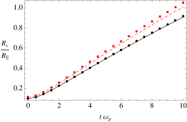
(a) Prolate shape ($\lambda=0.1$).

(b) Spherical shape ($\lambda=1$).

Figure 1: (Color online) Comparison of the free expansion for $\gamma=800$ using the variational method and the the direct numerical simulation of GPE. The lines and marks come from the variational method and the numerical simulation of GPE, respectively. Full line and circle mark (black color) correspond to $\ell=0$, and the dashed line and square mark (red color) correspond to $\ell=2$.

IV Results and Discussions

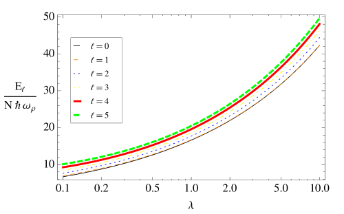
Figure 2: (Color online) Energy plotted as function of the trap anisotropy for different vortex circulations. The dimensionless interaction parameter is taken as $\gamma=800$. This corresponds to a condensate with $10^{5}$ atoms and s-wave scattering length $a_{s}=100a_{0}$.

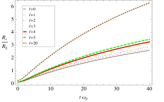
(a) $\lambda=0.1$

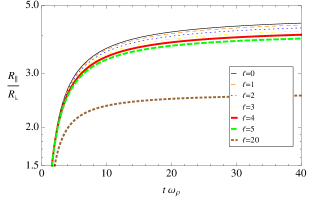
(b) $\lambda=10$

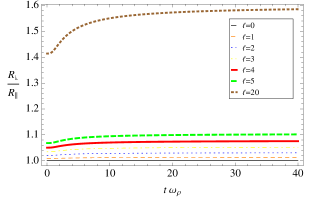
(c) $\lambda=1$

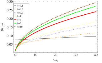
(d) $\ell=1$

Figure 3: (Color online) Aspect ratio evolution during free expansion for the respective trapped shapes: (a) prolate, (b) oblate and (c) spherical. They were calculated for $\gamma=800$. Frame (d) represents the ratio between the vortex core and the radial radius during the expansion for several kind of trap shapes.

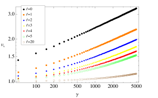
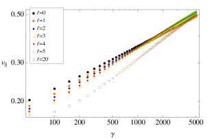
(a) $\lambda=0.1$

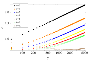
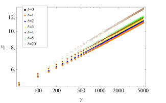
(b) $\lambda=10$

Figure 4: (Color online) The asymptotic behavior of expansion velocities as a function of $\gamma$ for initially prolate (a) and oblate (b) shapes.

The initial condition for the variational parameters where calculated from Eqs. (16) and (17) considering the radial frequency $\omega_{\rho}=2\pi\times 207Hz$. The time evolution of the parameters was obtained by numerically solving Eqs. (18) and (19) using the fourth-order adaptive Runge-Kutta method, with expansion times of the order of $30ms$. These values where chosen in order to be consistent with our experiments using ⁸⁷Rb 87 atoms de Lima Henn (2008).

Figure 2 shows the initial energy of the system for a fixed interaction parameter as function of the trap anisotropy measured by the parameter $\lambda$. It shows the monotonic growth of the condensate energy with the circulation of the vortex due to the extra kinetic energy and the larger volume occupied by the condensate with increasing $\ell$.

The vortex core evolution was analyzed considering its size to be given by Eq. (8). A disadvantage of this method comes from the fact that the static constraint (8) between the vortex core and the cloud dimensions is considered to be also valid during the entire expansion time. At least in principle, our Ansatz can be improved by introducing an additional parameter which characterizes the core expansion independently. In practice, the introduction of such an additional parameter affecting the density profile of the cloud is a not a trivial task. Indeed, the phase of the condensate wave function must also be modified in order to reproduce superfluid current corresponding to the time-variant core size. However, since in this work our attention is restricted to static configurations and the expansion of the cloud, the approach used here work turns out to be appropriate as we can see from Fig. 1.

In Fig. 3(a)–(c), the time evolution of the aspect ratio for different trap configurations and vortex circulations is depicted. Figure 3(c) shows how the growth of the dimensions of the cloud during the expansion are affected by the circulation of the central vortex. The higher the circulation of these vortices, the greater is the anisotropy introduced in the cloud shape. This effect is further increased during the cloud expansion.

In prolate condensates, Fig. 3a shows that the circulation has the effect of decreasing the time for the aspect ratio inversion due to the larger velocity field in the plane perpendicular to the vortex line before the expansion. In the opposite case, where the initial geometry is oblate, as in Fig. 3b, the circulation increases the time required for aspect ratio inversion.

In this work, the expansion of the vortex core is analyzed by evolving both the radial and axial radius using Eqs. (18) and (19), and then calculating the radius $\xi$ of the vortex according to (8). By taking the asymptotic solutions of Eqs. (18) and (19), it was also possible to extract the asymptotic expansion velocities along the radial and axial directions, as shown in Fig. 4. These information supply a method for determining the presence as well as the circulation of central vortices in an asymmetric cloud by simply looking at the asymptotic expansion velocities, which would require the repetition of the experiment considering different expansion time. An alternative method relies on dependence of the expansion dynamics on the circulation $\ell$ as depicted in Fig. 3d. In fact, Figs. 3(a)–(c) give a one to one correspondence between the aspect ratio of the expanded cloud and the multiplicity of the central vortex. This way, the multiplicity of the central core can be determined from aspect ratio obtained from time-of-flight pictures.