On Inefficiency of Markowitz-Style Investment
Strategies When Drawdown is Important

Abstract

The focal point of this paper is the issue of “drawdown” which arises in recursive betting scenarios and related applications in the stock market. Roughly speaking, drawdown is understood to mean drops in wealth over time from peaks to subsequent lows. Motivated by the fact that this issue is of paramount concern to conservative investors, we dispense with the classical variance as the risk metric and work with drawdown and mean return as the risk-reward pair. In this setting, the main results in this paper address the so-called “efficiency” of linear time-invariant (LTI) investment feedback strategies which correspond to Markowitz-style schemes in the finance literature. Our analysis begins with the following principle which is widely used in finance: Given two investment opportunities, if one of them has higher risk and lower return, it will be deemed to be inefficient or strictly dominated and generally rejected in the marketplace. In this framework, with risk-reward pair as described above, our main result is that classical Markowitz-style strategies are inefficient. To establish this, we use a new investment strategy which involves a time-varying linear feedback block $K(k)$, called the drawdown modulator. Using this instead of the original LTI feedback block $K$ in the Markowitz scheme, the desired domination is obtained. As a bonus, it is also seen that the modulator assures a worst-case level of drawdown protection with probability one.

I INTRODUCTION

The focal point of this paper is the issue of drawdown which arises in recursive betting scenarios and related applications in the stock market; i.e., we consider drops in wealth over time from peaks to subsequent lows. Given that this issue is of paramount concern to conservative investors or bettors, instead of using the classical variance as the risk metric, we use the drawdown. Accordingly, our risk-reward pair is obtained using this quantity in combination with the expected return. Beginning with this motivation, in the sequel, we study issues of “efficiency” which arise when linear feedback control strategies are used to adjust the time-varying investment levels $I(k)$ which are selected at each stage. In the sequel, our understanding is that $I(k)$ denotes either an “investment” or “bet.” We use these two terms interchangeably.

The Markowitz and Kelly strategies, in their simplest form, for example see [1]-[3], tell us that the investment $I(k)$ at each stage $k$ should be “proportional-to-wealth.” To be more precise, if $V(k)$ is the account value of an investor or bettor at stage $k$, then such a strategy is described by time-invariant feedback

$$I(k)=KV(k)$$

where the constant $K$ which represents the proportion of the account wagered. We also refer to $I(k)$ above as a Markowitz-style investment function. Typically, when selecting the constant $K$, we include constraints which we express as $K\in\mathcal{K}.$ When $\cal{K}$ includes negative numbers, this is interpreted to mean that short selling is allowed. In this case, $I(k)<0$ indicates that the investor is taking the “opposite side” of the trade or bet being offered. An important example is the case $\mathcal{K}=[-1,1]$. In this case, $|I(k)|\leq V(k)$ and that the investment is said to be cash-financed.

The type of LTI feedback control scheme described above is not only important here but central to our earlier work in [4]-[9]. To see the control-theoretic set-up more clearly, see Figure I. In the figure, the $X(k)$ are independent and identically distributed random variables representing return from the $k$-th investment $I(k)$ and the associated gain or loss is $I(k)X(k)$. For the short-selling case, a profit results when $X(k)<0$.

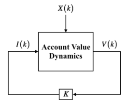
Figure 1: Markowitz-Style Gambling Feedback Configuration

The Notion of Inefficiency: The analysis to follow begins with the following principle which is widely used in finance: Given two investment opportunities, if one of them has larger risk and lower return, it will be deemed to be inefficient and generally rejected in the marketplace. Such an inefficient scheme is said to be “strictly dominated.” We also refer to a strategy being “dominated” when the inequalities associated with these conditions are not necessarily strict. As previously stated, in the literature, the most classical choice for the risk-reward pair is the variance and expected return; e.g., see [1], [2] and [10]. While the use of this pair is quite useful, it relies on an assumption that the returns are normally distributed. Thus, if the distribution of returns is skewed, then the use of such risk-return metric may be misleading; e.g., see [8], [9] and [11] for more detailed discussion.

More importantly, as far as this paper is concerned, as previously indicated, instead of using the classical variance as the risk metric when studying efficiency, we use drawdown of wealth which is important from a risk management perspective. Suffice it to say, the issue of drawdown has received a considerable attention in the finance literature; e.g., see [12]-[18]. Of these papers, references [15] and [16] are most relevant. Although their problem setup and assumptions differ from ours, they include one basic idea which is central to our modulation controller described below: The investment level is dynamically controlled as a function of “drawdown to date.” With the above providing context, our new results on efficiency to follow are based on maximum percentage drawdown and expected return as the risk-reward pair.

Main Results in This Paper: To study efficiency, we work with a new feedback-control which generalizes the Markowitz-style investment scheme. This new control includes a constant gain $\gamma$ and a block $M(\cdot)$ called the drawdown modulator which was introduced in [7]; see Figure I. With the aid of the modulator block, we show that it is possible to “dominate” a Markowitz-style strategy; i.e., we obtain the same expected drawdown and higher expected return. This is made possible by the fact that the modulator $M(\cdot)$ includes memory of $V(0),V(1),...,V(k-1)$ whereas a classical Markowitz-style investment strategy $I(k)=KV(k)$ is memoryless. In addition to our main result on domination described above, as a “bonus,” we also see that the modulator assures a prescribed level of worst-case drawdown protection which is guaranteed with probability one.

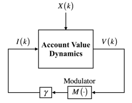
Figure 2: Drawdown-Modulated Feedback Configuration

II CLASSICAL DRAWDOWN CONCEPTS

Consistent with the body of existing literature on drawdown, the definition which we use is as follows: For $k=0,1,2,...,N$, we let $V(k)$ be the corresponding account value. Then, as $k$ evolves, the percentage drawdown to-date is defined as

$$d(k)\doteq\frac{V_{\max}(k)-V(k)}{V_{\max}(k)}$$

where

$$V_{\max}(k)\doteq\max_{0\leq i\leq k}V(i).$$

This leads to the overall maximum percentage drawdown

$$d^{*}\doteq\max_{0\leq k\leq N}d(k)$$

which is central to the analysis to follow. Note that $0\leq d^{*}\leq 1.$ Although not considered in this paper, there is another well-known drawdown-based measure, called the maximum absolute drawdown. The reader is referred to [12] and [13] for work on this topic.

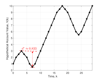
Figure 3: Maximum Percentage Drawdown

Illustration of Drawdown Definition: To further elaborate on the notion of drawdown, we consider an example with a hypothetical account value $V(k)$ shown in Figure II. From the plot, the overall maximum percentage drawdown

$$d^{*}=\frac{3-0.5}{3}\approx 0.833$$

occurs at stage $k=7.$ Note that this maximum percentage drawdown is not necessarily equal to the maximum absolute drawdown which has value $4.5$ and occurs at stage $k=24.$ Percentage drawdown is often used in lieu of absolute drawdown so that the scale of betting is taken into account.

III INVESTMENT DETAILS AND EFFICIENCY

In this section, the classical Markowitz-style investment scheme is described in more detail. To begin, for $k=0,1,2,...,N-1$, we let $X(k)$ be independent and identically distributed (i.i.d.) random variables which represent returns for a sequence of sequential bets. We assume that $X_{\min}\leq X(k)\leq X_{\max}$ with $X_{\min}$ and $X_{\max}$ being points in the support, denoted by $\mathcal{X}$, and satisfying $X_{\min}<0<X_{\max}.$ Recalling the discussion in Section I, the $k$-th investment is given by $I(k)\doteq KV(k).$ To assure that the feedback gain $K$ guarantees $V(k)\geq 0$ for all $k$, we require that

$$-\frac{1}{{{X_{\max}}}}\leq K\leq\frac{1}{{\left|{{X_{\min}}}\right|}}$$

be satisfied. The reader is referred to [6] for more details on this condition. It is also important to note that the $I(k)<0$ is allowed above; i.e., per Section I, short selling is admissible. That is, $I(k)>0$ leads to a profit when $X(k)>0$ and $I(k)<0$ leads to a profit when $X(k)<0$. Now beginning at initial account value $V(0)>0$, the evolution to terminal state $V(N)$ is described sequentially by the recursion

$$V(k+1) =V(k)+I(k)X(k)$$

$$=(1+KX(k))V(k).$$

This leads to terminal account value

$$V\left(N\right)=\prod\limits_{k=0}^{N-1}{\left({1+KX(k)}\right)V(0)}$$

which is useful for calculation of the overall return in the sections to follow. Although not the focal point of this paper, it is noted that there are many possibilities for selection of the feedback gain $K$ above. Among these possibilities, a popular criterion for selection of $K$ requires maximizing the expected logarithmic growth of wealth; e.g., see [3], [5], [6], [19] and [20].

Efficiency Considerations: The question now arises regarding the extent to which a Markowitz-style investment scheme is efficient. Indeed, against any sample path $X(k)$, we let $R_{K}$ denote the overall return; i.e.,

$$R_{K} \doteq\frac{V(N)-V(0)}{V(0)}=\prod\limits_{k=0}^{N-1}{\left({1+KX\left(k\right)}\right)}-1$$

and along the path, we obtain

$$d_{K}^{*}\doteq\max_{0\leq k\leq N}d_{K}(k)$$

which is the maximum percentage drawdown. Note that the subscript $K$ in $R_{K}$ and $d_{K}^{*}$ is used to emphasize the dependence on the feedback gain $K$. Now, to study efficiency, in the sections to follow, we use the expected values of $R_{K}$ and $d_{K}^{*}$ below. Using the shorthand

$$\overline{\vrule height=0.0pt\fontcharht\A+.2exwidth0ptR}_{K}\doteq\mathbb{E}[R_{K}]$$

and

$$\overline{\vrule height=0.0pt\fontcharht\A+.2exwidth0ptd}^{{}_{*}}_{K}\doteq\mathbb{E}[d_{K}^{*}]$$

to denote these quantities, we obtain the attainable risk-return performance curve in the plane as

$$\{{(\overline{\vrule height=0.0pt\fontcharht\A+.2exwidth0ptR}_{K},\overline{\vrule height=0.0pt\fontcharht\A+.2exwidth0ptd}^{{}_{*}}_{K}):K\in\mathcal{K}}\}.$$

In addition, recalling that $X(k)$ are independent and identically distributed, letting $\mu\doteq\mathbb{E}[X(k)]$ and using the formula for $R_{K}$ above, we obtain

$$\overline{\vrule height=0.0pt\fontcharht\A+.2exwidth0ptR}_{K} = \mathbb{E}\left[{\prod\limits_{k=0}^{N-1}{\left({1+KX\left(k\right)}\right)}}\right]-1\hfill$$

$$= {\left({1+K\mathbb{E}\left[{X\left(k\right)}\right]}\right)^{N}}-1$$

$$= {\left({1+K\mu}\right)^{N}}-1.$$

As far as calculation of $\overline{d}_{K}^{{}_{*}}$ is concerned, except for small values of $N$, Monte-Carlo simulations are used to calculate this quantity; see Section VI for more detail. Further to $\overline{d}_{K}^{{}_{*}}$, it is straightforward to see that the worst-case percentage drawdown is

$$d^{*}\doteq 1-(1-|K|\max\{|X_{\min}|,X_{\max}\})^{N}$$

which is much less useful than $\overline{\vrule height=0.0pt\fontcharht\A+.2exwidth0ptd}_{K}^{{}_{*}}$ since it corresponds to losing every bet and typically has very low probability. For example, for a simple even-money payoff coin-flipping gamble with $N=10$ and probability of heads $P(X(k)=1)=p=0.6$, the celebrated Kelly optimum $K=2p-1=0.2$ obtained in papers such as [3] and [20], leads to $d^{*}=1-(1-0.2)^{10}\approx 0.89$ which corresponds to $89\%$ as the worst-case.

IV DRAWDOWN MODULATION

The starting point for this section is the fact that the classical Markowitz-style investment strategy above is “memoryless.” That is, at stage $k$, the investment $I(k)$ does not depend on $V(0),V(1),...,V(k-1)$. We now describe how the inclusion of a “modulator block,” first introduced in [7], can be used to improve performance when the risk metric is percentage drawdown. As shown below, this is a time-varying generalization of the linear feedback scheme $I(k)=KV(k)$. To begin, given a prescribed constant  $0<d_{\max}<1$ which represents the maximum allowable percentage drawdown, the following lemma plays an important in our theory. It provides a necessary and sufficient condition for any investment strategy $I(k)$ assuring that $d(k)\leq d_{\max}$ with probability one. For the sake of self-containment of this paper, we include the proof from [7] here.

The Drawdown Modulation Lemma: An investment function $I(\cdot)$ guarantees maximum acceptable drawdown level $d_{\max}$ or less with probability one if and only if the condition,

$$-\frac{{{d_{\max}}-d(k)}}{{\left({1-d\left(k\right)}\right){X_{\max}}}}V(k)\leq I(k)\leq\frac{{{d_{\max}}-d(k)}}{{\left({1-d\left(k\right)}\right)\left|{{X_{\min}}}\right|}}V(k)$$

is satisfied along all sample pathes.

Proof: To prove necessity, assuming that $d(k)\leq d_{\max}$ for all $k$ with probability one, we must show the required condition on $I(k)$ holds along all sample pathes. Indeed, letting $k$ be given, since both $d(k)\leq d_{\max}$ and $d(k+1)\leq d_{\max}$ with probability one, we claim this forces the required inequalities on $I(k)$. Without loss of generality, we provide a proof of the rightmost inequality for the case $I(k)\geq 0$ and note that a nearly identical proof is used for $I(k)<0$. Indeed, using the fact that $X_{\min}$ is in the support $\cal X$, there exists a suitably small neighborhood of $X_{\min}$, call it $\mathcal{N}(X_{\min})$, such that

$$P\left(X(k)\in\mathcal{N}(X_{\min})\right)>0.$$

Thus, given any arbitrarily small $\varepsilon>0$, there exists some point $X_{\varepsilon}(k)<0$ such that $X_{\varepsilon}(k)\in\mathcal{N}_{\varepsilon}(X_{\min}),$ $|X_{\min}-X_{\varepsilon}(k)|<\varepsilon$ and leading to associated realizable loss $I(k)|X_{\varepsilon}(k)|$. Noting that $V_{\max}(k+1)=V_{\max}(k)$ and

$$d(k+1)=d(k)+\frac{{\left|{{X_{\varepsilon}(k)}}\right|I(k)}}{{{V_{\max}}(k)}}\leq d_{\max}$$

we now substitute

$${V_{\max}}(k)=\frac{{V\left(k\right)}}{{1-d\left(k\right)}}>0$$

into the inequality above and noting that $|X_{\varepsilon}(k)|\to|X_{\min}|$ as $\varepsilon\to 0$, we obtain

$$I(k)\leq\frac{{{d_{\max}}-d(k)}}{{\left({1-d\left(k\right)}\right)\left|{{X_{\min}}}\right|}}V(k).$$

To prove sufficiency, we assume that the condition on $I(k)$ holds along all sample pathes. We must show $d(k)\leq d_{\max}$ for all $k$ with probability one. Proceeding by induction, for $k=0$, we trivially have $d(0)=0\leq d_{\max}$ with probability one. To complete the inductive argument, we assume that $d(k)\leq d_{\max}$ with probability one, and must show $d(k+1)\leq d_{\max}$ with probability one. Without loss of generality, we again provide a proof for the case $I(k)\geq 0$ and note that a nearly identical proof is used for $I(k)<0$. Now, by noting that

$$d\left({k+1}\right) =1-\frac{{V\left({k+1}\right)}}{{{V_{\max}}\left({k+1}\right)}},$$

and $V_{\max}(k)\leq V_{\max}(k+1)$ with probability one, we split the argument into two cases: If $V_{\max}(k)<V_{\max}(k+1)$, then $V_{\max}(k+1)=V(k+1).$ Thus, we have $d(k+1)=0\leq d_{\max}.$ On the other hand, if $V_{\max}(k)=V_{\max}(k+1)$, with the aid of the dynamics of account value, we have

$$d\left({k+1}\right) =1-\frac{{V\left(k\right)+I\left(k\right)X\left(k\right)}}{{{V_{\max}}\left(k\right)}}$$

$$\leq 1-\frac{{V\left(k\right)-I\left(k\right)\left|{{X_{\min}}}\right|}}{{{V_{\max}}\left(k\right)}}$$

Using the rightmost inequality condition on $I(k)$, we obtain $d\left({k+1}\right)\leq{d_{\max}}$ which completes the proof. $\;\;\;\;\;\square$

Drawdown-Modulated Feedback Control: Motivated by the lemma above, we now consider a time-varying feedback control of the form

$$I(k)=K(k)V(k)$$

with $K(k)=\gamma M(k)$ where

$$M(k)\doteq\frac{d_{\max}-d(k)}{1-d(k)}$$

and

$$-\frac{1}{{{X_{\max}}}}\leq\gamma\leq\frac{1}{{|{X_{\min}}|}}.$$

Note that $0\leq M(k)\leq d_{\max}$. In the sequel, the constraint above on $\gamma$ is denoted by writing $\gamma\in\Gamma$. In the next section, we see how the two design variables $d_{\max}\in(0,1)$ and $\gamma\in\Gamma$ are selected by the designer when we study the efficiency issue.

V THE DOMINATION LEMMA

We now show that with drawdown-modulated feedback, it is possible to “dominate” a Markowitz-style strategy; i.e., it leads to the same expected drawdown and possibly higher expected return. As a bonus, as previously stated, we also see that the modulator assures a pre-specified worst-case level of drawdown protection with probability one.

Attainable Risk-Return Performance: Henceforth, we use notation

$$\mathcal{M}\doteq(\gamma,d_{\max})\in\Gamma\times(0,1)$$

to denote an admissible drawdown modulation pair. Then, the associated return and maximum percentage drawdown is denoted by $R_{\mathcal{M}}$ and $d_{\mathcal{M}}^{*}$, respectively. Hence, for the expected return and expected maximum drawdown, we write

$$\overline{\vrule height=0.0pt\fontcharht\A+.2exwidth0ptR}_{\mathcal{M}}\doteq\mathbb{E}[R_{\mathcal{M}}]$$

and

$$\overline{\vrule height=0.0pt\fontcharht\A+.2exwidth0ptd}_{\mathcal{M}}^{{}_{*}}\doteq\mathbb{E}[d_{\mathcal{M}}^{*}].$$

This leads to the attainable risk-return performance set in the plane described by

$$\left\{{\left({{{\overline{\vrule height=0.0pt\fontcharht\A+.2exwidth0ptR}}_{\mathcal{M}}},\overline{\vrule height=0.0pt\fontcharht\A+.2exwidth0ptd}_{\mathcal{M}}^{{}_{*}}}\right):\mathcal{M}\doteq(\gamma,d_{\max})\in\Gamma\times(0,1)}\right\}.$$

To obtain points in the set above, we use an idea which is found in the celebrated Markowitz risk-return theory in finance; e.g., see [1] and [2]. That is, given any target level of expected drawdown, call it $\widehat{d}$, we seek an admissible pair $\mathcal{M}\doteq(\gamma,d_{\max})\in\Gamma\times(0,1)$ maximizing $\overline{\vrule height=0.0pt\fontcharht\A+.2exwidth0ptR}_{\mathcal{M}}$ subject to the constraint $\overline{\vrule height=0.0pt\fontcharht\A+.2exwidth0ptd}_{\mathcal{M}}^{{}_{*}}=\widehat{d}.$ In our case, this is found by solving a two-dimensional optimization over the rectangle constraining $\gamma$ and $d_{\max}$ above. We are now prepared to address the issue of domination.

The Domination Lemma: For any admissible $K\in\mathcal{K}$, there exists a drawdown modulator pair $\mathcal{M}=(\gamma,d_{\max})$ such that

$$\overline{\vrule height=0.0pt\fontcharht\A+.2exwidth0ptR}_{\mathcal{M}}\geq\overline{\vrule height=0.0pt\fontcharht\A+.2exwidth0ptR}_{K}$$

and

$$\overline{\vrule height=0.0pt\fontcharht\A+.2exwidth0ptd}_{\mathcal{M}}^{{}_{*}}=\overline{\vrule height=0.0pt\fontcharht\A+.2exwidth0ptd}_{K}^{{}_{*}}.$$

Proof: To begin, taking the target level of drawdown $\widehat{d}\doteq\overline{d}_{K}^{*}$, we must show that there is an admissible pair $\mathcal{M}=(\gamma,d_{\max})$ which leads to $\overline{\vrule height=0.0pt\fontcharht\A+.2exwidth0ptd}_{\mathcal{M}}^{{}_{*}}=\widehat{d}$ and $\overline{\vrule height=0.0pt\fontcharht\A+.2exwidth0ptR}_{\mathcal{M}}\geq\overline{\vrule height=0.0pt\fontcharht\A+.2exwidth0ptR}_{K}.$ Indeed, taking $\gamma=K$ and letting $d_{\max}\to 1$, we first replicate the performance of Markowitz-style investment scheme; i.e., we obtain $\overline{\vrule height=0.0pt\fontcharht\A+.2exwidth0ptd}_{\mathcal{M}}^{{}_{*}}=\overline{\vrule height=0.0pt\fontcharht\A+.2exwidth0ptd}_{K}^{{}_{*}}$ and $\overline{\vrule height=0.0pt\fontcharht\A+.2exwidth0ptR}_{\mathcal{M}}=\overline{\vrule height=0.0pt\fontcharht\A+.2exwidth0ptR}_{K}.$ Hence the maximization of $\overline{\vrule height=0.0pt\fontcharht\A+.2exwidth0ptR}_{\mathcal{M}}$ over all admissible $\mathcal{M}\in\Gamma\times(0,1)$ with constraint $\overline{\vrule height=0.0pt\fontcharht\A+.2exwidth0ptd}_{\mathcal{M}}^{{}_{*}}=\overline{\vrule height=0.0pt\fontcharht\A+.2exwidth0ptd}_{K}^{{}_{*}}$ must be at least as large as $\overline{\vrule height=0.0pt\fontcharht\A+.2exwidth0ptR}_{K}.$  $\square$

Remarks: Note that the Markowitz-style strategy can be viewed as a subclass of drawdown-modulated class obtained with $\gamma=K$ and $d_{\max}\to 1$. Furthermore, as demonstrated in the Section VI, it is typically the case that the inequality in the lemma above is “strict.” In other words, the Markowitz-style investment scheme may be “strictly dominated” by a strategy in the modulator class.

VI ILLUSTRATIVE EXAMPLES

In many applications, the broker’s constraint on leverage forces the satisfaction of the cash-financing condition $|I(k)|\leq V(k)$; i.e., for drawdown modulated feedback, to guarantee this condition is satisfied, the constraint on $\gamma$ described in Section IV is augmented to include $|\gamma|\;M(k)\leq 1.$ Similarly, for a Markowitz-style investment strategy, to guarantee the cash financing condition, we augment the constraint on $K$ to include $|K|\leq 1.$ In the examples to follow the constraint which we impose on the Markowitz-style investment is also used for the modulation scheme.

We now illustrate use of our result on domination via examples. We begin with the simple case when $N=2$ where calculations can be carried out in closed form. Then we study the more general scenario with $N>2$ where Monte Carlo simulation is used. Indeed, for $N=2$, we consider a single coin-flipping gamble having even-money payoff described by independent and identically distributed random variables $X(k)\in\{-1,1\}$ and $P(X(k)=1)\doteq p>1/2$.

Reward-Risk Calculations for Both Schemes: Now, beginning with $\mu=\mathbb{E}[X(k)]=2p-1$, for the Markowitz-style betting strategy with parameter $K>0$, the associated expected return is readily calculated to be

$$\overline{\vrule height=0.0pt\fontcharht\A+.2exwidth0ptR}_{K} ={\left({1+K\left({2p-1}\right)}\right)^{2}}-1.$$

and the expected maximum percentage drawdown, found by a straightforward calculation is given by

$$\overline{\vrule height=0.0pt\fontcharht\A+.2exwidth0ptd}^{{}_{*}}_{K} =K(1-p)\left({2-K+Kp}\right).$$

For drawdown modulator pair $\mathcal{M}\doteq(\gamma,d_{\max})$, a lengthy but straightforward computation leads to expected return and expected maximum percentage drawdown given by

$$\overline{\vrule height=0.0pt\fontcharht\A+.2exwidth0ptR}_{\mathcal{M}} =\gamma{d_{\max}}(2p-1)(\gamma{d_{\max}}p+\gamma p-\gamma+2)$$

and

$$\overline{\vrule height=0.0pt\fontcharht\A+.2exwidth0ptd}_{\mathcal{M}}^{{}_{*}} =\gamma{d_{\max}}\left({1-p}\right)\left({2-\gamma+\gamma p}\right).$$

Demonstration of Strict Domination: Now, we establish “strict domination” using drawdown-modulated feedback strategy. That is, for any $0<K<1$, we prove that there exists a modulator $\mathcal{M}=(\gamma,d_{\max})$ such that $\overline{\vrule height=0.0pt\fontcharht\A+.2exwidth0ptR}_{K}<\overline{\vrule height=0.0pt\fontcharht\A+.2exwidth0ptR}_{\mathcal{M}}^{{}_{*}}$ and $\overline{\vrule height=0.0pt\fontcharht\A+.2exwidth0ptd}_{\mathcal{M}}^{{}_{*}}=\overline{\vrule height=0.0pt\fontcharht\A+.2exwidth0ptd}_{K}^{{}_{*}}.$ Indeed, to prove this, it is sufficient to take $\gamma=1$ and

$${d_{\max}}=\frac{{K\left({2-K+Kp}\right)}}{{1+p}}$$

which is obtained by setting $\overline{\vrule height=0.0pt\fontcharht\A+.2exwidth0ptd}_{\mathcal{M}}^{{}_{*}}=\overline{\vrule height=0.0pt\fontcharht\A+.2exwidth0ptd}_{K}^{{}_{*}}$ above. It is readily verified that $0<d_{\max}<1$ and by substitution of $d_{\max}$ and $\gamma$ into $\overline{\vrule height=0.0pt\fontcharht\A+.2exwidth0ptR}_{\mathcal{M}}$, after a lengthy but straightforward calculation, we obtain

$${\overline{\vrule height=0.0pt\fontcharht\A+.2exwidth0ptR}_{\mathcal{M}}}=\frac{{K(2p-1)(2-K+Kp)f\left({K,p}\right)}}{{{{(1+p)}^{2}}}}$$

where $f(K,p)\doteq 2Kp-{K^{2}}p+{K^{2}}{p^{2}}+{p^{2}}+2p+1.$ Now, to establish the desired domination, we now claim that $\overline{\vrule height=0.0pt\fontcharht\A+.2exwidth0ptR}_{\mathcal{M}}>\overline{R}_{K}.$ To prove this, we show that the difference between left and right hand sides above is positive. Indeed, via a lengthy but straightforward calculation, we obtain

$$\overline{R}_{\mathcal{M}}-\overline{R}_{K} =\frac{{{K^{2}}(1-K)(1-p)p(2p-1)(3+p+Kp-K)}}{{{{(1+p)}^{2}}}}.$$

Noting that $0<K<1$ and $p>1/2$ above, it is immediate that both numerator and denominator for the difference described above are strictly positive. Thus, $\overline{\vrule height=0.0pt\fontcharht\A+.2exwidth0ptR}_{\mathcal{M}}>\overline{\vrule height=0.0pt\fontcharht\A+.2exwidth0ptR}_{K}.$ To complete this analysis, in Figure VI we provide a plot which shows the degree of the strict domination in the difference based on our calculation of $\overline{\vrule height=0.0pt\fontcharht\A+.2exwidth0ptR}_{\mathcal{M}}-\overline{R}_{K}$ above.

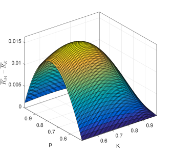
Figure 4: Degree of Strict Domination in Expected Return

Example of Inefficiency with Larger $N$: Again, we consider a single coin-flipping scenario with even-money payoff described by independent and identically distributed random variables $X(k)\in\{-1/30,1/30\}$ and $P(X(k)=1/30)=0.6$ with corresponding mean $\mu=\mathbb{E}[X(k)]=1/{150}.$ We choose $N=252$ and view this as a trading problem for a binomial stock-price model over one year with daily returns varies around $\pm 3.3\%$ corresponding to $X(k)=1/30$ above. Note that this scenario is more biased on $X(k)=1/30$. Hence, we study efficiency for the case when $0\leq K\leq 1$.

Demonstration of Inefficiency: For the Markowitz scheme, we first obtain the expected return

$$\overline{\vrule height=0.0pt\fontcharht\A+.2exwidth0ptR}_{K} ={\left({1+\frac{K}{{150}}}\right)^{252}}-1.$$

As far as the expected maximum percentage drawdown $\overline{d}_{K}^{{}_{*}}$ is concerned, this quantity is computed via performing a large number of Monte-Carlo simulations. Our finding is that for $0\leq K\leq 1,$ we have $\overline{\vrule height=0.0pt\fontcharht\A+.2exwidth0ptd}_{K}^{{}_{*}}\approx 0.25K.$ For the drawdown-modulated feedback with the cash-financing condition imposed, to certify inefficiency, we proceed as follows: As previously discussed in Section IV, for a given target level of drawdown $\widehat{d}\in(0,1)$, we seek to find a pair $\mathcal{M}=(\gamma^{*},d_{\max})$ maximizing $\overline{\vrule height=0.0pt\fontcharht\A+.2exwidth0ptR}_{\mathcal{M}}$ subject to $\overline{\vrule height=0.0pt\fontcharht\A+.2exwidth0ptd}_{\mathcal{M}}^{{}_{*}}=\widehat{d}.$ This two-parameter optimization is solved with a large Monte-Carlo simulation. Then, letting $\overline{\vrule height=0.0pt\fontcharht\A+.2exwidth0ptR}_{\mathcal{M}}^{{}_{*}}(\widehat{d})$ denote the approximate optimal value obtained, we generate the dotted line in the Figure VI. We see that for any given risk level, the drawdown-modulated feedback leads to a certifiably higher expected return than the Markowitz-style investment scheme. In other words, the Markowitz-style investment scheme is “strictly dominated” as seen in the figure.

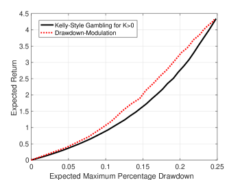
Figure 5: Risk-Reward Efficiency Plot for $N=252$

VII CONCLUSION AND FUTURE WORK

In this paper, using expected maximum percentage drawdown and mean return as the risk-reward pair, we demonstrated inefficiency of Markowitz-style investment schemes. This was accomplished using our so-called drawdown-modulated feedback control. In addition, as a bonus, this controller was seen to guarantee a prescribed level of drawdown protection with probability one. By way of extending the results given in this paper, it is interesting to note that a drawdown-modulated controller can be used to obtain very similar domination results for other return metrics as well. For example, if $\overline{\vrule height=0.0pt\fontcharht\A+.2exwidth0ptR}_{K}$ is replaced by the expected logarithmic growth $\mathbb{E}[\log(V(N)/V(0)])$, which is central to papers such as [3], [5], [6], [19] and [20], performance comparisons are obtained which are very similar to that given in Figure VI result.

Regarding further research on efficiency issues, one obvious extension would be to consider a portfolio case which involves many correlated random variables; i.e., we take $X(k)$ to be a vector rather than the scalar considered here. When $X(k)$ has dimension $n$ which is large, finding the attainable performance curve, often called the efficient frontier, may require an algorithm aimed at dealing with high computational complexity. Another interesting problem for future research is motivated by the fact that the feedback gain for our drawdown-modulated feedback scheme we used is simply a pure gain $\gamma$. It may prove to be the case that a time-varying feedback gain $\gamma(k)$ may lead to superior performance in the risk-reward efficiency framework. Finally, as seen in Section V, the lemma does not guarantee “strict” domination. An interesting extension of this work would be to provide conditions under which strictness can be guaranteed.

References

- [1] H. Markowitz, “Portfolio Selection,” The Journal of Finance, vol 7, pp. 77-91, 1952
- [2] H. Markowitz, Portfolio Selection: Efficient Diversification of Investments, Yale University Press, 1968.
- [3] J. L. Kelly, “A New Interpretation of Information Rate,” Bell System Technical Journal, vol 35.4, pp. 917-926, 1956.
- [4] B. R. Barmish and J. A. Primbs, “On a New Paradigm for Stock Trading Via a Model-Free Feedback Controller,” IEEE Transactions on Automatic Control, AC-61, pp. 662-676, 2016.
- [5] C. H. Hsieh and B. R. Barmish, “On Kelly Betting: Some Limitations,” Proceedings of the Allerton Conference on Communication, Control, and Computing, pp. 165-172, Monticello, 2015.
- [6] C. H. Hsieh, B. R. Barmish and J. A. Gubner, “Kelly Betting Can be Too Conservative,” Proceedings of the IEEE Conference on Decision and Control, pp. 3695-3701, Las Vegas, 2016.
- [7] C. H. Hsieh and B. R. Barmish, “On Drawdown-Modulated Feedback in Stock Trading,” IFAC-PapersOnLine, vol. 50, no. 1 pp. 952-958, 2017.
- [8] S. Malekpour and B. R. Barmish, “How Useful are Mean-Variance Considerations in Stock Trading via Feedback Control,” Proceedings of the IEEE Conference on Decision and Control, Maui, pp. 2110-2115, 2012.
- [9] S. Malekpour and B. R. Barmish, “A Drawdown Formula for Stock Trading Via Linear Feedback in a Market Governed by Brownian Motion,” Proceedings of the European Control Conference, Zurich, Switzerland, pp. 87-92, 2013.
- [10] Z. Bodie, A. Kane and A. Marcus, Investments, McGraw-Hill, 2010.
- [11] D. G. Luenberger, Investment Science, Oxford University Press, New York, 2011.
- [12] M. Ismail, A. Atiya, A. Pratap and Y. Abu-Mostafa, “On the Maximum Drawdown of a Brownian Motion,” Journal of Applied Probability, vol. 41, pp. 147-161, 2004.
- [13] B. T. Hayes, “Maximum Drawdowns of Hedge Funds with Serial Correlation,” Journal of Alternative Investments, vol. 8, pp. 26-38, 2006.
- [14] L. R. Goldberg and O. Mahmoud, “Drawdown: From Practice to Theory and Back Again,” Mathematics and Financial Economics, pp. 1-23, 2016.
- [15] S. J. Grossman and Z. Zhou, “Optimal Investment Strategies for Controlling Drawdowns,” Mathematical Finance, vol. 3, pp. 241-276, 1993.
- [16] J. Cvitanic and I. Karatzas, “On Portfolio Optimization Under Drawdown Constraints,” IMA Lecture Notes in Mathematics and Applications, vol. 65, pp. 77-88, 1994.
- [17] A. Chekhlov, S. Uryasev and M. Zabarankin, “Portfolio Optimization with Drawdown Constraints,” Asset and Liability Management Tools, ed. B. Scherer, Risk Books, pp. 263-278, 2003.
- [18] A. Chekhlov, S. Uryasev and M. Zabarankin. “Drawdown Measure in Portfolio Optimization,” International Journal of Theoretical and Applied Finance vol 8, pp.13-58, 2005.
- [19] L. C. MacLean, E. O. Thorp, and W. T. Ziemba, The Kelly Capital Growth Investment Criterion: Theory and Practice, World Scientific Publishing Company, 2011.
- [20] E. O. Thorp, “The Kelly Criterion in Blackjack Sports Betting and The Stock Market,” Handbook of Asset and Liability Management: Theory and Methodology, vol. 1, pp. 385-428, Elsevier Science, 2006.