Efficient Parallel Solution of the 3D Stationary Boltzmann Transport Equation for Diffusive Problems

Abstract

This paper presents an efficient parallel method for the deterministic solution of the 3D stationary Boltzmann transport equation applied to diffusive problems such as nuclear core criticality computations. Based on standard MultiGroup-Sn-DD discretization schemes, our approach combines a highly efficient nested parallelization strategy [1] with the PDSA parallel acceleration technique [2] applied for the first time to 3D transport problems. These two key ingredients enable us to solve extremely large neutronic problems involving up to $10^{12}$ degrees of freedom in less than an hour using 64 super-computer nodes.

1 Introduction

This paper presents an efficient parallel deterministic solution of the stationary Boltzmann Transport Equation (BTE) applied to 3D diffusive problems.

1.1 Deterministic 3D stationary Boltzmann transport equation solver

The BTE governs the statistical evolution of gas-like collections of neutral particles described by phase-space densities $f(\vec{r},\vec{p},t)$ proportional to the number of particles at a position $\vec{r}$, with momentum $\vec{p}$ at a given time $t$. This one-body description is widely used to simulate the transport of particles like neutrons or photons through inhomogeneous reactive media. The material properties of the media are characterized by cross-sections that measure the probability of various particle interactions: absorption, diffusion, emission, etc.

Lying in a six-dimensional (6D) space (3 for space and 3 for momentum), a precise mesh-based discretization of the stationary BTE solutions $f(\vec{r},\vec{p})$ can be very large for true 3D cases where the considered physical problem offers no particular spatial symmetry. As an example, using a Cartesian 6D Mesh with 100 points per axis leads to $10^{12}$ phase-space cells which contain several Degrees Of Freedom (DOFs). Considering the scale of a BTE solution, one can easily infer that its solving procedure may rapidly exhaust the capability of the largest supercomputers. As a consequence, probabilistic methods (Monte-Carlo) that avoid the phase-space mesh problems, were the only approaches able to deal with true 3D cases until the beginning of this century. Unfortunately, probabilistic methods converge slowly with the number $N$ of pseudo-particles ($\propto N^{-1/2}$) and the computational demand increases strongly with the desired accuracy. During the last two decades the peak performance of super-computers has been multiplied by a factor of $10^{4}$. Modern supercomputer capabilities have made deterministic methods a credible alternative to probabilistic methods for 3D problems and has allowed for unprecedented accuracy levels for BTE approximate solutions.

1.2 Reference criticality computations for nuclear diffusive problems

BTE solvers are used in different physical contexts and optimal numerical methods differ from one application to another. In this paper we address the specific problem of solving the stationary BTE in diffusive media. Diffusive problems arise when the mean-free path of particles becomes small compared to the characteristic scale of the considered problem. For such media, and considering an optically thick enough geometry, one may neglect the advective part of the transport and replace the original BTE by the much simpler diffusion equation.

This work takes place in the context of nuclear reactor simulations. We consider the transport of neutrons inside nuclear reactor cores which contain optically thick diffusive media. More specifically, we address the problem of nuclear core criticality computations. Because nuclear cross-sections mainly depend on the particle energy, the phase-space density variable $f(\vec{r},\vec{p})$ is replaced by the angular neutron flux $\psi(\vec{r},E,\vec{\Omega)}=vf(\vec{r},\vec{p})$ where $\vec{\Omega}$ stands for the particle momentum direction, $v$ its velocity and $E$ its kinetic energy. Nuclear operators need to complete many criticality computations that correspond to stationary BTE solutions. Industrial routine computations, which are primarily used to conduct operational and safety studies and to optimize nuclear reactor core designs, are often based on the diffusion equation approximation. In order to assess this approximation, the solution of the original BTE problem is required. More generally, nuclear operators need accurate reference transport solutions in order to control the accuracy of their simulations.

1.3 Starting from a classical numerical scheme

The proposed method is based on nested algorithms classically used for nuclear criticality computations. The external loop is a Chebyshev accelerated Power Iteration (PI) that solves the eigenvalue problem $H\psi=k^{-1}F\psi$ where $H$ is the transport operator and $F$ the fission operator. The kinetic energy of neutrons is discretized in well chosen slices called energy groups and, for each PI iteration, an iterative Gauss-Seidel (GS) algorithm is used to solve the multigroup linear problem. For each energy group, the angular variable is treated with the discrete ordinates method ($S_{N}$) and a Source Iteration (SI) algorithm deals with the coupling between angular components of the flux. For diffusive problems the SI procedure converges slowly and is classically accelerated by the Diffusion Synthetic Acceleration method (DSA) [3]. In this paper, we introduce a parallel extension of the DSA method (PDSA) where an efficient single-domain diffusion solver is required. Finally, the space is discretized over 3D Cartesian meshes, and all the examples of the paper use the lowest order Diamond Differencing spatial discretization scheme (DD0), which appears to be efficient for diffusive nuclear core simulations [4]. Note that the PDSA method does not depend on the DD0 choice and a higher order numerical scheme could have been used. The only condition is that these alternative schemes must be consistent with the single-domain DSA solver.

1.4 New metrics for efficient numerical algorithms

The tremendous peak power of modern supercomputers, that commonly exceeds $10^{16}$ floating point operations per second (FLOPS), is accompanied by a high architecture complexity. Indeed, recent architectures exhibit a hierarchical organization (cluster of nodes of multicore processors with vector units) which requires a mix of different parallel programming paradigms (Message Passing, Multi-Threading, SIMD) to achieve optimal efficiency. In addition to this mixture of parallel programming models, a new constraint on the data movements has emerged and plays a dominant role in computation efficiency. A direct consequence of this machine evolution is that numerical algorithms should no longer be evaluated upon their parallel scalability ($i$) alone. The computational density ($ii$) which measures the ratio between the number of floating point (FP) operations and the number of data movements from the off-chip memory to CPU registers is a new metric that must be considered to evaluate the efficiency of a given algorithm. Finally, the vectorization potential ($iii$) of a given algorithm will determine its ability to benefit from the ever increasing Single Instruction Multiple Data (SIMD) width of dedicated CPU FP SIMD instructions (SSE2, AVX, AVX512). The combination of these three algorithm characteristics ($i$,$ii$,$iii$) will eventually result in an efficient numerical solver. In this paper we put a particular focus on the efficiency of the proposed BTE solver and explain how parallel scalability, computational density and vectorization potential are taken into account.

1.5 Paper contributions

In this paper we propose a parallel and efficient solution method for the stationary BTE that allows one to carry out very large criticality computations for diffusive problems on moderately large supercomputers. These affordable full 3D transport computations result from an uncommonly high effective FP performance that can exceed 20% of the available theoretical peak performance of the computing nodes. As a representative example, we show that a 3D PWR $k_{\text{eff}}$ computation with 26 energy groups, 288 angular directions, and $578\times 578\times 140$ space cells, can be completed in less than an hour using 64 cluster nodes. Two main ingredients are combined in the proposed method that has been implemented in Domino [5, 6], our in-house neutron transport solver.

• A very high performance sweep algorithm including 3 nested levels of parallelism with good data locality and fine grained synchronization that has been described in detail in [1].

• A novel scalable PDSA acceleration technique for diffusive problem introduced in [2] and applied for the first time to 3D transport computations. This method is easy to implement provided a fast single-domain shared-memory diffusion solver. Hence PDSA allows one to avoid the complex task of building fully distributed diffusion solvers as implemented in [7, 8].

Recently, important progress has been made for increasing the scalability of BTE solvers. In [9] the authors replace the Power Iterations by advanced eigenvalue algorithms and treat the energy groups in parallel. The scalability of this approach is impressive and parallel computations involving more than $10^{5}$ computing cores are presented. In this current paper we show that, for a moderately high number of groups ($\leq$ 26), the proposed method results in fast criticality computations with more modest numbers of computing cores ($10^{2}-10^{3}$) thereby making 3D stationary computation more affordable.

This result should have an impact on the acceleration strategies for other kinds of BTE solvers like unstructured mesh based transport solvers or the accelerated Monte-Carlo approach for criticality nuclear computations.

The paper is organized as follows. In Section 2, we describe the equations to be solved, the different discretization schemes, the main algorithm and the three nested levels of parallelism used in the sweep implementation described in [1]. In Section 3, the PDSA algorithm and its implementation are described and some details are given regarding the correct coupling between the Transport DD0 discretization and the Finite Element method used in the PDSA. Section 4 describes the parallel performance achieved by Domino for different PWR criticality computation configurations. Some conclusions and outlooks are given in section 5.

2 The Discrete Ordinates Method for Neutron Transport Simulation

2.1 Source Iterations Scheme

We consider the monogroup transport equation as defined in equation (1).

$$\begin{split}\underbrace{\vv\Omega\cdot\vv\nabla\psi(\vv r,\vv\Omega)+\Sigma_{t}(\vv r,\vv\Omega)\psi(\vv r,\vv\Omega)}_{L\psi(\vv r,\vv\Omega)}-\overbrace{\int_{S_{2}}{d\vv\Omega^{\prime}}\Sigma_{s}(\vv r,\vv\Omega^{\prime}\cdot\vv\Omega)\psi(\vv r,\vv\Omega^{\prime})}^{R(\vv r,\vv\Omega)}=Q(\vv r,\vv\Omega),\end{split}$$ (1)

where $Q(\vv r,\vv\Omega)$ gathers both monogroup fission and inter-group scattering sources. The angular dependency of this equation is resolved by looking for solutions on a discrete set of carefully selected angular directions {$\vv\Omega_{i}\in S_{2}$, $i=1,2,\cdots,N_{\text{dir}}$}, called discrete ordinates; each one being associated to a weight $w_{j}$. In general, the discrete ordinates are determined thanks to a numerical quadrature formula as defined in equation (2). For any summable function $g$ over $S_{2}$:

$$\bar{g}\equiv\int_{S_{2}}g(\vv\Omega)d\vv\Omega\simeq\sum_{j=1}^{N_{\text{dir}}}w_{j}g(\vv\Omega_{j}).$$ (2)

In Domino, we use the Level Symmetric [10] quadrature formula, which leads to $N_{\text{dir}}=N(N+2)$ angular directions, where $N$ stands for the Level Symmetric quadrature formula order.

Therefore, considering that the cross-sections are isotropic, equation (1) becomes:

$$\begin{split}\vv\Omega_{i}\cdot\vv\nabla\psi(\vv r,\vv\Omega_{i})+\Sigma_{t}(\vv r)\psi(\vv r,\vv\Omega_{i})=\overbrace{Q(\vv r,\vv\Omega_{i})+\Sigma_{s}(\vv r)\phi(\vv r)}^{S(\vv r,\vv\Omega_{i})},\end{split}$$ (3)

where $\phi(\vv r)$ is the scalar flux and defined by:

$$\phi(\vv r)\equiv\bar{\psi}(\vv r,\cdot)=\int_{S_{2}}\psi(\vv r,\vv\Omega)d\vv\Omega\simeq\sum_{j=1}^{N_{\text{dir}}}w_{j}\psi(\vv r,\vv\Omega_{j}).$$ (4)

Equation (3) is solved by iterating over the scattering source as described in Algorithm 1.

Input : $\phi^{k}$

Output : $\phi^{k+\frac{1}{2}}$

while Non convergence do

       for $i=1,\dots,N_{\text{dir}}$ do

             $S(\vv r,\vv\Omega_{i})=Q(\vv r,\vv\Omega_{i})+\Sigma_{s}(\vv r)\phi^{k}(\vv r)$;

            3 $L\psi^{k+\frac{1}{2}}(\vv r,\vv\Omega_{i})=S(\vv r,\vv\Omega_{i})$;

             $\phi^{k+\frac{1}{2}}(\vv r)=\sum_{j=1}^{N_{\text{dir}}}w_{j}\psi^{k+\frac{1}{2}}(\vv r,\vv\Omega_{j})$;

            

      

Algorithm 1 Source iterations

Each source iteration (SI) involves the resolution of a fixed-source problem (Line 1), for every angular direction. This is done by discretizing the spatial variable $\vv r$ of the streaming operator $L$. In this work, we focus on a $3$D reactor core model, represented by a $3$D Cartesian domain $\mathcal{D}$, and $L$ is discretized using a Diamond Difference scheme (DD), as presented by A. Hébert in [11]. The discrete form of the fixed-source problem is then solved by “walking” step by step throughout the whole spatial domain and to progressively compute angular fluxes in the spatial cells. In the literature, this process is known as the sweep operation. The vast majority of computations performed in the ${\sc S_{\text{N}}}$ method are part of the sweep operation.

2.2 Sweep Operation

The sweep operation is used to solve the space-angle problem on Line 1 of Algorithm 1. It computes the angular neutron flux inside all cells of the spatial domain, for a set of angular directions. These directions are grouped into four quadrants in 2D (or eight octants in 3D). In the following, we focus on the first quadrant (labeled I in Figure 1a). As shown in Figure 1b explanation, each cell has two incoming dependencies $\psi_{L}$ and $\psi_{B}$ for each angular direction. At the beginning, incoming fluxes on all left and bottom faces are known as indicated in Figure 1c. Hence, the cell $(0,0)$ located at the bottom-left corner is the first to be processed. The treatment of this cell allows for the updating of outgoing fluxes $\psi_{R}$ and $\psi_{T}$, that satisfy the dependencies of cells $(0,1)$ and $(1,0)$. These dependencies on the processing of cells define a sequential nature throughout the progression of the sweep operation: two adjacent cells belonging to successive diagonals cannot be processed simultaneously. However, all cells belonging to a same diagonal can be processed in parallel. Furthermore, treatment of a single cell for all directions of the same quadrant can be done in parallel. Hence, step by step, fluxes are evaluated in all cells of the spatial domain, for all angular directions belonging to the same quadrant. The same operation is repeated for all the four quadrants. When using vacuum boundary conditions, there are no incoming neutrons to the computational domain and therefore processing of the four quadrants can be done concurrently. This sweep operation is subject to numerous studies regarding design and parallelism to reach highest efficiency on parallel architectures.

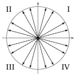
(a) Angular quadrature in 2D. Directions are grouped in quadrants.

(b) In each direction, cells have two incoming components of the flux (Here, from the left and bottom faces: $\psi_{L}$ and $\psi_{B}$), and generates two outgoing components of the flux (Here, on the right and top faces: $\psi_{R}$ and $\psi_{T}$).

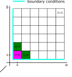
(c) Domain decomposition and boundary conditions. The corner cell $(0,0)$ is the first to be processed for a quadrant, and its processing then allows for the processing of its neighbors (Here $(0,1)$ and $(1,0)$).

Figure 1: Illustration of the sweep operation over a $6\times 6$ 2D spatial grid for a single direction.

2.3 Hierarchical Parallelization of the Sweep

In this section, we briefly describe the parallelization of the ${\sc S_{\text{N}}}$-sweep operation on distributed multicore-based architectures. A detailed description of the Domino’s ${\sc S_{\text{N}}}$-sweep can be found in [1] and [12].

As one can see from Figure 1, a space cell $c_{i,j}$ with Cartesian indices $i$ and $j$ can be processed as soon as both cells $c_{i-1,j}$ and $c_{i,j-1}$ have been computed. In order to reduce the cost of parallel communications, we do not consider individual cells but group them into MacroCells $C_{I,J}$ that correspond to rectangular sets of cells. Let $T_{I,J}$ be the task corresponding to the sweep inside a MacroCell $C_{I,J}$. The dependency between all the tasks:

$$(T_{I-1,J},T_{I,J-1})\rightarrow T_{I,J}$$

defines a Directed Acyclic Graph (DAG) which corresponds to the complete sweep from one corner of the spatial mesh to the opposite corner. An illustration of this DAG is presented in Figure 2a.

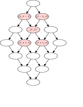
(a) A 2D single-quadrant Sweep’s DAG over a 4x4 grid of MacroCells.

(b) Snapshot of an execution of the Sweep operation implemented on top of PaRSEC. MacroCells of similar colors are processed on the same node and highlighted ones are those that are in the process of being executed (at the time the snapshot was taken).

Figure 2: Sweep’s DAG and snapshot.

This DAG description, the task implementation and the data distribution over the computing nodes, are passed to a parallel runtime system. Here, we choose the PaRSEC [13] runtime system and its specific parameterized task graph to describe the algorithm. This format corresponds well with the regular pattern of our regular domain decomposition and allows the runtime system to schedule the tasks in a fully distributed manner without discovering integrally the graph of dependencies. In practice, PaRSEC exploits this pattern regularity to automatically schedule all computations on a set of threads per node (usually one thread per core), and triggers communications through an MPI layer when necessary. A snapshot of the execution on top of PaRSEC is depicted in Figure 2b.

In the case of vacuum boundary conditions, all 4 (resp. 8) angular sweep quadrants (resp. octants) are processed in parallel and again, handled via PaRSEC.

Finally, each task $T_{I,J}$ exhibits a third innermost level of parallelism based on Single Instruction Multiple Data (SIMD). SIMD capabilities of modern computing cores allow them to perform, at each clock cycle, several identical floating point operations ($+$,$*$,…) on different floating point values. This SIMD parallelism is used to perform the sweep operations that correspond to different angular directions of the same quadrant inside each spatial cell. A detailed description of this vectorized implementation based on Eigen, a C++ template library, can be found in [6].

3 Acceleration of Scattering Iterations using PDSA

In highly diffusive media ($\Sigma_{s}\approx\Sigma_{t}$), the convergence of Algorithm 1 is very slow, and therefore a numerical acceleration scheme must be combined with this algorithm in order to speed-up its convergence. One of the widely used acceleration schemes in this case, is Diffusion Synthetic Acceleration (DSA) [14].

3.1 Diffusion Synthetic Acceleration

Here we just recall the basics of this method, and the reader can refer to the paper [14] for more details regarding its effectiveness and the Fourier analysis characterizing its convergence properties. Let us define $\epsilon^{k+\frac{1}{2}}=\psi-\psi^{k+\frac{1}{2}}$, as the error of the solution obtained after the $k+\frac{1}{2}^{\text{th}}$ iteration of the SI scheme, relative to the exact solution $\psi$, as defined by equation (3). The error $\epsilon$ satisfies the following transport equation:

$$L\epsilon^{k+\frac{1}{2}}(\vv r,\vv\Omega_{i})=\Sigma_{t}(\vv r)\bar{\epsilon}^{k+\frac{1}{2}}+\Sigma_{s}(\vv r)\displaystyle\left(\phi^{k+\frac{1}{2}}(\vv r)-\phi^{k}(\vv r)\right),$$ (5)

where $\bar{\epsilon}$ is the scalar field associated to $\epsilon$ and defined as in equation (2). However, equation (5) is as difficult to solve as the original fixed-source transport problem (3). Nevertheless, if an approximation $\tilde{\epsilon}$ of $\bar{\epsilon}$ was available, then the scalar flux could be updated to:

$$\phi^{k+1}(\vv r)=\phi^{k+\frac{1}{2}}(\vv r)+\tilde{\epsilon}^{k+\frac{1}{2}}(\vv r).$$

The idea of the DSA method is then to use a diffusion approximation, yielding $\tilde{\epsilon}$, instead of solving the transport equation (5). In Domino, the diffusion approximation is obtained using the Diabolo solver [15], which implements the simplified ${\sc P_{\text{N}}}$ (${\sc SP_{\text{N}}}$) method as presented in [16], in a mixed-dual formulation. When approximating equation (5) with a diffusion operator, the problem solved by Diabolo can be stated as the following mixed dual formulation:

Find $$(\tilde{\epsilon}^{k+\frac{1}{2}},\vv j^{k+\frac{1}{2}})\in L^{2}(\mathcal{D})\times H(\mathcal{D},\operatorname{div})$$ such that:

$$\quad\left\{\begin{aligned} &\operatorname{div}\vv j^{k+\frac{1}{2}}(\vv r)+\Sigma_{a}\tilde{\epsilon}^{k+\frac{1}{2}}(\vv r)=\Sigma_{s}(\vv r)\displaystyle\left(\phi^{k+\frac{1}{2}}(\vv r)-\phi^{k}(\vv r)\right)&\text{in}~{}\mathcal{D},\\ &\frac{1}{D}\vv j^{k+\frac{1}{2}}(\vv r)+\vv{\nabla}\;\tilde{\epsilon}^{k+\frac{1}{2}}(\vv r)=\vv 0&\text{in}~{}\mathcal{D},\\ &\tilde{\epsilon}^{k+\frac{1}{2}}=0&\text{on}~{}\partial\mathcal{D},\end{aligned}\right.$$ (6)

in which we introduced the diffusion coefficient $D$ and the neutronic current $\vv j^{k+\frac{1}{2}}$ associated to $\tilde{\epsilon}^{k+\frac{1}{2}}$. Within Diabolo, these equations are spatially discretized using an RTk finite elements scheme [17, 18] (see Figure 3), which is consistent with the DD scheme used for the discretization of the transport equation as proven in [11]. Therefore, the stability of the acceleration scheme is ensured.

Figure 3: RT0 finite element in 2D: $5$ DoFs ($4$ for the currents $J_{x}$, $J^{\prime}_{x}$, $J_{y}$, $J^{\prime}_{y}$ and $1$ for the scalar flux $\phi$). DSA is applied using an RT0 element.

However, when integrated into a parallelized transport solver, DSA may become a bottleneck for the scalability of the transport solver if, for instance, a serial implementation of the diffusion solver is used. On the other hand, if the diffusion solver is parallelized, as presented in [7, 8] using a domain decomposition method, the iteration count to the solution increases with the number of subdomains, and can lead to a poor global scalability [19]. To remedy this issue, a variant of the DSA scheme has been recently proposed by F. Févotte in [2].

3.2 Piecewise Diffusion Synthetic Acceleration

The general presentation and the convergence proof of the Piecewise Diffusion Synthetic Acceleration (PDSA) method are given in [2]. We recall that the purpose of this method is similar to that of DSA: evaluate an approximation, $\tilde{\epsilon}^{k+\frac{1}{2}}$, of the error on the scalar flux, $\bar{\epsilon}^{k+\frac{1}{2}}$, to be used for correcting the scalar flux, $\phi^{k+\frac{1}{2}}$. In the following, iteration indices $k+\frac{1}{2}$ will be dropped for the sake of readability.

We assume that the spatial domain $\mathcal{D}$ is split, along the $3$ spatial dimensions, into $N=P\times Q\times R$ non-overlapping subdomains $\mathcal{D}_{I}$ such that: $\mathcal{D}=\cup_{I\in\mathcal{I}}\mathcal{D}_{I}$, where

$$\mathcal{I}=\llbracket 1,P\rrbracket\times\llbracket 1,Q\rrbracket\times\llbracket 1,R\rrbracket.$$

We set: $\Gamma_{IJ}=\partial\mathcal{D}_{I}\cap\partial\mathcal{D}_{J}$ the non-empty interfaces between subdomains of index $I$ and $J$; $\Gamma_{I}=\partial\mathcal{D}\cap\partial\mathcal{D}_{I}$ and $\mathbf{n}_{I}$ the unit normal vector to $\partial\mathcal{D}_{I}$ and $\tilde{\epsilon}^{I}=\tilde{\epsilon}|_{\mathcal{D}_{I}}$ and $\vv j^{I}=\vv j|_{\mathcal{D}_{I}}$, the respective restrictions of $\tilde{\epsilon}$ and $\vv j$ to subdomain $\mathcal{D}_{I}$.

Unlike the DSA method which consists in solving a single ${\sc SP_{\text{N}}}$ problem on the global domain $\mathcal{D}$, the PDSA method is based on successive resolutions of two ${\sc SP_{\text{N}}}$ problems on each of the subdomains $\mathcal{D}_{I}$. These ${\sc SP_{\text{N}}}$ problems differ on the boundary conditions applied on the subdomains: the first problem uses homogeneous Neumann boundary conditions (equation (7)), and the second one uses non-homogeneous Dirichlet boundary conditions (equation (8)). In both equations, notations were shortened by using $S^{I}(\vv r)$ to denote the right-hand side of equation (6).

$$\left\{\begin{aligned} &\operatorname{div}\vv j_{N}^{I}(\vv r)+\Sigma_{a}\tilde{\epsilon}_{N}^{I}(\vv r)=S^{I}(\vv r)&\text{in}~{}\mathcal{D}_{I}\\ &\vv{\nabla}\;\tilde{\epsilon}_{N}^{I}(\vv r)+\frac{1}{D}\vv j_{N}^{I}(\vv r)=\vv 0&\text{in}~{}\mathcal{D}_{I}\\ &\tilde{\epsilon}_{N}^{I}=0&\text{on}~{}\Gamma_{I}\\ &\vv\nabla\tilde{\epsilon}_{N}^{I}\cdot\mathbf{n}_{I}=0&\text{on}~{}\Gamma_{IJ}\end{aligned}\right.$$ (7)

$$\left\{\begin{aligned} &\operatorname{div}\vv j_{D}^{I}(\vv r)+\Sigma_{a}\tilde{\epsilon}_{D}^{I}(\vv r)=S^{I}(\vv r)&\text{in}~{}\mathcal{D}_{I}\\ &\vv{\nabla}\;\tilde{\epsilon}_{D}^{I}(\vv r)+\frac{1}{D}\vv j_{D}^{I}(\vv r)=\vv 0&\text{in}~{}\mathcal{D}_{I}\\ &\tilde{\epsilon}_{D}^{I}=0&\text{on}~{}\Gamma_{I}\\ &\tilde{\epsilon}_{D}^{I}=\frac{\tilde{\epsilon}_{N}^{I}+\tilde{\epsilon}_{N}^{J}}{2}&\text{on}~{}\Gamma_{IJ}\end{aligned}\right.$$ (8)

As shown in [2], for sufficiently diffusive and optically thick problems, the PDSA solution $\tilde{\epsilon}_{D}$ is an approximation of the global DSA solution $\tilde{\epsilon}$. The accelerated ${\sc S_{\text{N}}}$ flux is thus finally given by:

$$\phi^{k+1}=\phi^{k+\frac{1}{2}}+\tilde{\epsilon}_{D}.$$

On the practical side, it is important to note that the application of the PDSA method using a classical diffusion solver does not require many changes. Homogeneous Dirichlet boundary conditions used over $\Gamma_{I}$ are classically implemented to simulate whole cores; homogeneous Neumann boundary conditions used over $\Gamma_{IJ}$ in equation (7) are likewise featured by most diffusion solvers to implement symmetric domains. However, the second PDSA step (8) requires implementing a non-homogeneous Dirichlet boundary condition, which is not standard. In our case we are using a mixed-dual formulation of the ${\sc SP_{\text{N}}}$ equations, therefore these boundary conditions are natural and not essential and their implementation is straightforward. An illustration of the processing of the boundary conditions in the case of two subdomains is presented in Figure 4.

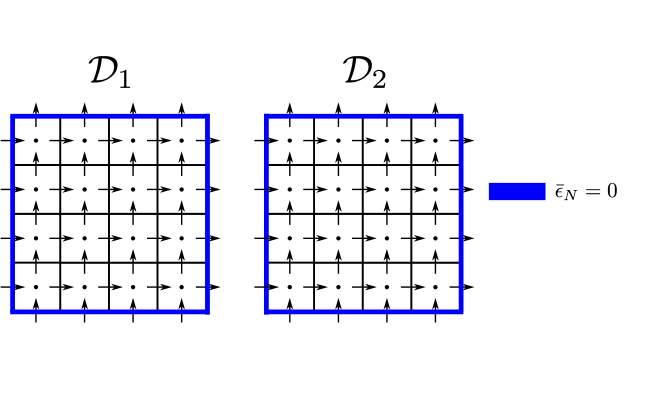
(a) The first step consists of solving two diffusion problems in parallel on $\mathcal{D}_{1}$ and $\mathcal{D}_{2}$, with Neumann boundary conditions.

(b) The second step also solves two diffusion problems, but with non-homogeneous Dirichlet boundary conditions: null flux boundary conditions on the external boundary of the domain and an average value of the flux at the inner interface.

Figure 4: Illustration of the PDSA method on a domain split in two.

This is a major shift from the classical DSA method, as we are no longer required to get the solution of the diffusion problem on the whole spatial domain. The first advantage of this method is that the explicit global synchronizations between the resolutions of the piecewise diffusion problems are largely reduced, hence allowing to fully parallelize the DSA method without efficiency loss. In addition, as we are going to see in section 4, the effectiveness of the PDSA method is comparable to that of the classical DSA method on a class of benchmarks.

3.3 Parallelization of the PDSA Method

Figure 5 illustrates a parallel implementation of the PDSA method in 2D, when the global domain is partitioned in two subdomains.

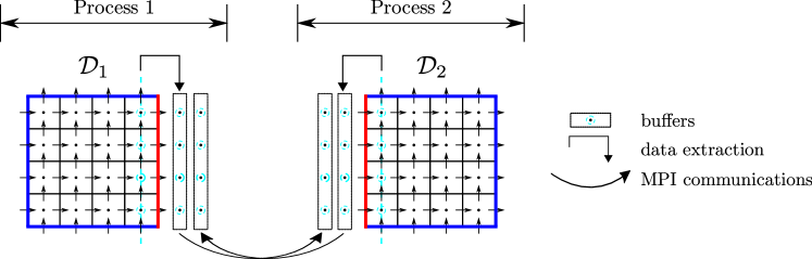
Figure 5: Illustration of the communication pattern in the PDSA method on a domain split in two. Two point-to-point communications are needed to exchange flux information at the interface between the two subdomains.

The partitioning of the global domain uses the same block data distribution as for the sweep operation. As we mentioned previously in section 3.1, the diffusion problem on each subdomain is solved using our ${\sc SP_{\text{N}}}$ solver Diabolo which is parallelized on shared memory systems using the Intel TBB framework.

Hence, by mapping each subdomain to a single process, the resolution of the diffusion problems on $\mathcal{D}_{1}$ and $\mathcal{D}_{2}$, when applying the PDSA method, is naturally performed in parallel. Moreover, for the first step, the use of Neumann boundary conditions requires no communication with the neighboring processes. However, in the second step, each process needs to have the average value of the scalar flux at the interfaces between its neighbors. Therefore, each process must perform send and receive operations to exchange data with its neighbors.

4 Performance of Domino

The performance and accuracy of the single-domain Domino implementation, based on standard DSA acceleration, has been assessed in [12] and [5] where comparisons with both reference Monte-Carlo and deterministic solvers have been conducted. In this section, we assess the performance of the present multi-domain Domino implementation based on the PDSA method for solving a set of PWR nuclear core benchmarks.

These benchmarks correspond to a PWR 900 MW core, and enable $2$, $8$ and $26$ energy groups calculations to be performed. A full description of these benchmarks is available in [20]. All benchmarks represent a simplified 3D PWR first core loaded with $3$ different types of fuel assemblies characterized by different Uranium-235 enrichment levels (low, medium and highly enriched uranium). There are no control rods inserted in this core model. Along the z-axis, the $360$ cm assembly is axially reflected with $30$ cm of water which results in a total core height of $420$ cm. The $3$ types of fuel assemblies appear on Figure 6a where the central assembly corresponds to the lowest enrichment, while the last row of fuel assemblies has the highest enrichment to flatten the neutron flux. Each fuel assembly is a $17\times 17$ array of fuel pins, with a lattice pitch of $1.26$ cm that contains $264$ fuel pins and $25$ water holes. The boundary condition associated with this benchmark problem is a pure leakage condition without any incoming angular flux. The associated nuclear data, $2$-group, $8$-group and $26$-group libraries are derived from a fuel assembly heterogeneous transport calculation performed with the cell code DRAGON [21]. As an example, figure 6b presents a visualization of the thermal flux in the central radial plane, as obtained from a 2-group calculation.

(a) Material Radial Map

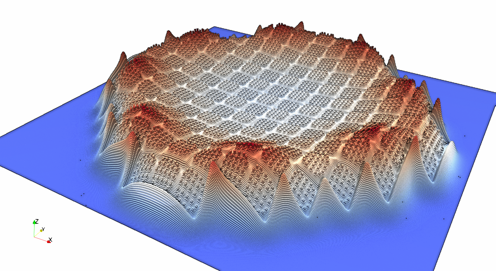
(b) Neutron Thermal Flux

Figure 6: Illustration of the 2-Group PWR 900 MW model [20]

Table 1 summarizes the discretization parameters for the considered benchmarks, where the following notations are used:

• ${N_{\text{G}}}$ is the number of energy groups.

• $N_{x}$, $N_{y}$ and $N_{z}$ define the number of spatial cells along the three dimensions of the spatial domain.

• $N_{\text{dir}}$ is the number of angular directions according to the order of angular quadrature in use.

• ${N_{\text{dof}}}$ is the number of degrees of freedoms (DoFs). The calculation of DoF numbers consider $3$ DoFs per cell, per energy group and per angular direction.

• Flops is the number of floating point operations required to perform a single complete sweep operation, for all energy groups. Note that the sweep of a single spatial cell for a single angular direction requires $25$ flops (see [1]).

• $A_{x}$, $A_{y}$ and $A_{z}$ define the MacroCell sizes along the three dimensions. Experimentally, $A_{x,y,z}=16$ was shown to be the most effective choice for the 2-group benchmark.

• $\epsilon_{k_{\text{eff}}}$ and $\epsilon_{\psi}$ define the thresholds used to check the stopping criteria at iteration $n+1$ of the power algorithm for the eigenvalue and on the fission source respectively as follows:

  $$\frac{|k_{\text{eff}}^{n+1}-k_{\text{eff}}^{n}|}{k_{\text{eff}}^{n}}<\epsilon_{k_{\text{eff}}},\quad\frac{||\mathcal{F}\psi^{n+1}-\mathcal{F}\psi^{n}||}{||\mathcal{F}\psi^{n}||}<\epsilon_{\psi}.$$ (9)

• $I_{g}$ is the fixed number of Gauss-Seidel iterations for the multigroup problem.

${N_{\text{G}}}$	$N_{x}$	$N_{y}$	$N_{z}$	$N_{\text{dir}}$	${N_{\text{dof}}}$	Flops	$A_{x,y,z}$	$\epsilon_{k_{\text{eff}}}$	$\epsilon_{\psi}$	$I_{g}$
					$\times 10^{12}$	$\times 10^{12}$
$2$	$578$	$578$	$756$	$168$	$0.254$	$2.12$	$16$	$10^{-6}$	$10^{-5}$	1
$8$	$578$	$578$	$168$	$80$	$0.108$	$0.90$	$20$	$10^{-5}$	$10^{-5}$	5
$26$	$578$	$578$	$140$	$288$	$1.051$	$8.75$	$20$	$10^{-5}$	$10^{-5}$	4

Table 1: Description of PWR benchmarks and calculation parameters.

Note that the spatial mesh used for the PWR benchmarks is based on a pin-cell mesh in the $x-y$ plane. Each pin-cell is then subdivided into $70$ (resp. $84$) slices in the $z$ direction for the $26$-group (resp. $2$-group and $8$-group). The spatial mesh is then further refined by $2\times 2\times 2$ for the $8$-group and $26$-group, and by $2\times 2\times 9$ for the $2$-group. The larger spatial mesh for the $2$-group case enables the study of the strong scalability of our implementation at high core count.

The experiments have been conducted on computing nodes (dual Intel Xeon E5-2697v2 processors) of the athos cluster at EDF. The theoretical peak performance of each node is 518 (resp. 1036) GFlop/s in double (resp. single) precision ($2\times 12$ AVX cores at 2.7 GHz). The following experiments were conducted by launching one MPI process per computing node and as many threads as available cores; keeping one core per node for the PaRSEC communication thread. All experiments were conducted in single precision. Computation times do not include setup (reading of cross-section files from the hard disk), but include all communications and stopping criterion checks. For all the experiments presented in the following sections, the setup time is less than a minute.

4.1 Strong scalability of $2$-group PWR $k_{\text{eff}}$ computation

In this section, we present full-core $k_{\text{eff}}$ computations using the $S_{12}$ $2$-group 3D PWR core model. From a preliminary study with a single subdomain, we found that the optimal number of ${\sc SP_{\text{N}}}$ iterations is one, for each of the three benchmarks. Therefore, all the following results are obtained using this value.

Figure 7a compares the convergence of the standard DSA method with one subdomain $(P1,Q1,R1)$ and those of PDSA with $4$, $16$, $32$ and $64$ subdomains. All the computations lead to the same $k_{\text{eff}}$ (1.019574) and to the same fluxes. The outer iteration number increases from $56$ for one subdomain, to $71$ for $64$ subdomains. This small increase demonstrates that the PDSA method is a suitable parallel acceleration technique for PWR core problems. Table 2 summarizes these DSA and PDSA results and compares them to the non-accelerated computation which requires $315$ outer iterations to reach the convergence criterion. Figure 7b illustrates Domino’s strong scalability. The total computing time evolution and its main components are displayed. The ${\sc SP_{\text{N}}}$ time, which corresponds to the time dedicated to solving all the PDSA diffusion subproblems in all subdomains, scales perfectly and remains negligible for all the parallel range. The global parallel efficiency decrease is mainly due to the scalability limitation of the sweep. These results show that the PDSA method allows Domino to achieve very good performance for PWR criticality computations.

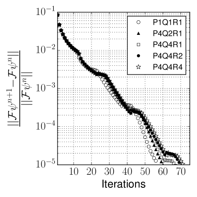
(a) PDSA convergence

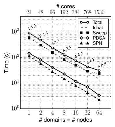
(b) PDSA timings

Figure 7: Convergence and elapsed CPU time of Domino using the $2$-group PWR benchmark for various multi-domain configurations. A $(P,Q,R)$ configuration divides the spatial domain in $P$ (resp. $Q$,$R$) slices in the $X$ (resp. $Y$,$Z$) direction.

($P$,$Q$,$R$)		$(1,1,1)$	$(1,1,1)$	$(4,2,1)$	$(4,4,1)$	$(4,4,2)$	$(4,4,4)$
Accel		No DSA	DSA	PDSA	PDSA	PDSA	PDSA
$N_{\text{cores}}$		$24$	$24$	$192$	$384$	$768$	$1536$
$N_{\text{outer}}$		315	$56$	$59$	$66$	$69$	$71$
${T_{\text{sweep}}}$	(s)	3610	$598.0$	$83.2$	$50.0$	$29.4$	$23.5$
${T_{\text{spn}}}$	(s)	-	$114.7$	$14.6$	$8.0$	$4.2$	$2.2$
$T_{\text{\tiny{Accel}}}$	(s)	-	$147.0$	$22.8$	$11.6$	$7.1$	$3.4$
${T_{\text{total}}}$	(s)	4547	$916.4$	$130.5$	$75.5$	$43.8$	$31.1$
$\%$ sweep		79	$65$	$64$	$66$	$67$	$75$

Table 2: Solution times for a $S_{12}$ $2$-group 3D PWR $k_{\text{eff}}$ computation on the athos platform.

The distributed memory nodes are efficiently used by this domain decomposition approach. Each multi-core node parallel potential is efficiently exploited by multi-threaded implementation of the sweep and mono-domain diffusion solvers. The core SIMD units, handling the third and innermost parallel level, are efficiently used to simultaneously compute several components of the angular flux. These three nested levels of parallelism allow Domino to exploit a large fraction of the computing power of the parallel platform. For this $S_{12}$ (resp. $S_{16}$) 2-group PWR Benchmark running on 768 cores, the performance of the sweep operation reaches 5.0 (resp. 6.6) TFlop/s which corresponds to $15\%$ (resp. $20\%$) of the peak performance of the corresponding 32 nodes.

4.2 PWR core mode with $8$ and $26$-groups

Table 3 presents performance results of $S_{8}$ $8$-group and $S_{16}$ $26$-group 3D PWR $k_{\text{eff}}$ computations using $64$ computing nodes of the athos cluster, partitioned into $(4,4,4)$.

3D PWR	$N_{\text{outer}}$	${T_{\text{sweep}}}$ (s)	${T_{\text{spn}}}$ (s)	$T_{\text{\tiny{PDSA}}}^{\text{comm}}$ (s)	${T_{\text{total}}}$ (s)
$S_{8}$ $8$-group	$65$	$91.53$	$7.84$	$0.86$	$128.85$
$S_{16}$ $26$-group	$126$	$2226.42$	$56.56$	$147.2$	$2763.52$

Table 3: Solution times for a $S_{12}$ $8$-group and $S_{16}$ $26$-group 3D PWR $k_{\text{eff}}$ computation on 64 cluster nodes (4,4,4).

The convergence on the 8-group benchmark is reached in $65$ external iterations, and the obtained eigenvalue is $k_{\text{eff}}=1.009408$. This number of external iterations is similar to what was obtained for a run with a single subdomain. The total computation time is $128.85$ s of which $91.53$ s comes from the sweep operation, illustrating that the sweep operation is still dominant ($71\%$ of the total time).

For the 26-group case, the convergence is reached in $126$ outer iterations, for a global solver time of $2763.52$ s. The obtained eigenvalue is $k_{\text{eff}}=1.008358$. As in the case with $8$-groups, we did not observe any increase in the number of external iterations as compared to a run with a single domain. This is a remarkable result, highlighting the perfect efficiency of the PDSA method on representative benchmarks of our target applications.

5 Conclusion

In this paper, we studied the performance of our massively parallel approach for solving the neutron transport equation according to the discrete ordinates method. We first presented our task-based implementation of the sweep with PaRSEC, as implemented in the Domino solver. Then we presented an application of PDSA, a new piecewise diffusion acceleration scheme for the scattering iterations. This is required to speed-up the convergence for strongly diffusive problems. The efficiency of the massively parallel PDSA approach has shown to be perfectly effective on different PWR nuclear core criticality computations where it matches the standard DSA convergence rate. The Cartesian transport solver Domino, implementing the PDSA scheme, exhibits three nested levels of parallelism and exploits a large fraction of the theoretical peak performance of thousands of SIMD computing cores. As a result, Domino can complete very large and accurate criticality computations involving more than $10^{12}$ degrees of freedom in less than an hour using 64 super-computer nodes.

This result allows us now to consider future fast and accurate 3D time-dependent transport solutions for diffusive problems.

References

- [1] S. Moustafa, M. Faverge, L. Plagne, P. Ramet, 3D Cartesian Transport Sweep for Massively Parallel Architectures with PaRSEC, in: Parallel and Distributed Processing Symposium (IPDPS), 2015 IEEE International, 2015, pp. 581–590. doi:10.1109/IPDPS.2015.75.
- [2] F. Févotte, PDSA: a piecewise diffusion synthetic acceleration scheme for neutron transport simulations in diffusive media, in preparation for submission to Journal of Computational Physics.
- [3] R. E. Alcouffe, Diffusion synthetic acceleration methods for the diamond-differenced discrete-ordinates equations, Nuclear Science and Engineering 64 (2) (1977) 344–355.
- [4] N. Martin, A. Hébert, A three-dimensional high-order diamond differencing discretization with a consistent acceleration scheme, Annals of Nuclear Energy 36 (11-12) (2009) 1787 – 1796. doi:10.1016/j.anucene.2009.08.014.
- [5] T. Courau, S. Moustafa, L. Plagne, A. Ponçot, DOMINO: A fast 3D Cartesian discrete ordiantes solver for reference pwr simulations and SPN validations, in: International Conference on Mathematics and Computational Methods Applied to Nuclear Science & Engineering (M&C 2013), USA, 2013.
-
[6]
S. Moustafa, I. Dutka-Malen, L. Plagne, A. Ponçot, P. Ramet,
Shared
memory parallelism for 3D Cartesian discrete ordinates solver, Annals of
Nuclear Energy 82 (2015) 179 – 187, joint International Conference on
Supercomputing in Nuclear Applications and Monte Carlo 2013, SNA + MC
2013. Pluri- and Trans-disciplinarity, Towards New Modeling and Numerical
Simulation Paradigms.
doi:http://dx.doi.org/10.1016/j.anucene.2014.08.034.
URL http://www.sciencedirect.com/science/article/pii/S0306454914004265 -
[7]
E. Jamelot, P. Ciarlet Jr,
Fast
non-overlapping Schwarz domain decomposition methods for solving the
neutron diffusion equation, Journal of Computational Physics 241 (2013) 445
– 463.
doi:http://dx.doi.org/10.1016/j.jcp.2013.01.026.
URL http://www.sciencedirect.com/science/article/pii/S0021999113000703 -
[8]
M. Barrault, B. Lathuilière, P. Ramet, J. Roman,