Two dimensional super QCD on a lattice

Abstract

We construct a lattice theory with one exact supersymmetry which consists of fields transforming in both the adjoint and fundamental representations of a U(Nc) gauge group. In addition to gluons and gluinos, the theory contains Nf flavors of fermion in the fundamental representation along with their scalar partners and is invariant under a global U(Nf) flavor symmetry. The lattice action contains an additional Fayet-Iliopoulos term which can be used to generate a scalar potential. We perform numerical simulations that corroborate the theoretical expectation that supersymmetry is spontaneously broken for Nf<Nc.

1 Introduction

A great deal of progress has occurred over the last decade in the construction of supersymmetric lattice theories. The key realization has been that in certain theories with extended supersymmetry it is possible to find linear combination(s) of the original supercharges that satisfy a nilpotent subalgebra of the full supersymmetry algebra which can be transferred intact to the lattice. The nature of this subalgebra is most clearly seen after the continuum theory is twisted - that is the theory is recast in a new set of variables that exposes a particular subgroup of the original global symmetries. This subgroup is the diagonal subgroup of the Lorentz and flavor symmetries - which are hence twisted or locked together. Details of these lattice constructions can be found in Sugino:2004qd ; Catterall:2004np ; physrep .  Initially the focus was on lattice actions that target pure super Yang-Mills theories in the continuum limit with a great deal of effort being devoted to ${\cal N}=4$ super Yang-Mills latsusy-1 ; latsusy-2 ; Catterall:2012yq ; Catterall:2011pd ; Catterall:2013roa .

In Matsuura and SuginoQuiver these formulations were extended using orbifold methods to the case of theories incorporating fermions transforming in the fundamental representation of the gauge group. These methods yield quiver gauge theories containing fields that transform as bi-fundamentals under a product gauge group $U(N_{c})\times U(N_{f})$.

In this work we derive these quiver actions by generalizing the existing twisted SYM lattice constructions in dimension $d+1$ to achieve a quiver theory and show how, in a certain limit, these reduce to a class of super QCD theory in dimension $d$. In practice we consider only the two dimensional case although it should be clear how this approach will generalize. We also discuss how to add a lattice supersymmetric Fayet-Illipoulos term to the action which will play a role in mediating spontaneous supersymmetry breaking. We have performed numerical simulations to test these ideas and our results show strong evidence for spontaneous susy breaking for $N_{f}<Nc$ as expected on general theoretical grounds.

2 Eight supercharge SYM on a 3d lattice

To target ${\cal N}=(2,2)$ SQCD in two dimensions we start from the continuum eight supercharge (${\cal Q}=8$) theory in three dimensions. Conventionally this is written as

$$S=\int d^{3}x\,\left(F_{ab}^{2}+\left(D_{a}B^{I}\right)^{2}+\left[B^{I},B^{J}\right]^{2}\right)+\;{\rm fermions}$$ (1)

Here the lowercase indices are spacetime indices while the uppercase indices denote flavor. All fields are in the adjoint representation of a $U(N_{c})$ gauge group $X=\sum_{a=1}^{N^{2}}X_{a}T_{a}$ and we will adopt an antihermitian basis for the generators $T_{a}$. After twisting this can be rewritten in terms of fields which are completely antisymmetric tensors in spacetime under the twisted SO(3) group given by

$$SO_{\rm twist}(3)={\rm diag}\left[SO_{\rm rot}(3)\times SO_{\rm flavor}(3)\right]$$ (2)

The original two Dirac fermions reappear in the twisted theory as the components of a Kähler-Dirac field $\Psi=\left(\eta,\psi_{a},\chi_{ab},\theta_{abc}\right)$. The bosonic sector of the twisted theory comprises a complexified gauge field ${\cal A}_{a}=A_{a}+iB_{a}$ containing the original gauge field $A_{a}$ and an additional vector field $B_{a}$. This additional field contains the original three scalars which, being vectors under the R symmetry, transform as the components of a vector field after twisting. The corresponding action $S=S_{\rm exact}+S_{\rm closed}$ becomes

$$S_{\rm exact} = \frac{1}{g^{2}}\;{\cal Q}\Lambda=\frac{1}{g^{2}}\;{\cal Q}\int d^{3}x{\rm Tr}\left[\chi_{ab}(x){\cal F}_{ab}(x)+\eta(x)\left[{\overline{\cal D}}_{a},{\cal D}_{a}\right]+\frac{1}{2}\eta(x)d(x)\right],$$ (3)

$$S_{\rm closed} = -\;\frac{1}{g^{2}}\int d^{3}x{\rm Tr}\left[\theta_{abc}(x){\overline{\cal D}}_{[c}\chi_{ab]}(x)\right].$$ (4)

where ${\cal D}_{a}$ and ${\overline{\cal D}}_{a}$ are the continuum covariant derivatives defined in terms of the complexified gauge fields as ${\cal D}_{a}=\partial_{a}+{\cal A}_{a}$ and ${\overline{\cal D}}_{a}=\partial_{a}+{\overline{\cal A}}_{a}$. The action of the scalar supersymmetry on the twisted fields is given by

$${\cal Q}{\cal A}_{a} = \psi_{a}$$

$${\cal Q}{\overline{\cal A}}_{a} = 0$$

$${\cal Q}\psi_{a} = 0$$

$${\cal Q}\chi_{ab} = -{\overline{\cal F}}_{ab}$$

$${\cal Q}\eta = d$$

$${\cal Q}\theta_{abc} = 0$$ (5)

Notice that we have included an auxiliary field $d(x)$ that allows the algebra to be off-shell nilpotent ${\cal Q}^{2}=0$. This feature then guarantees that $S_{\rm exact}$ is supersymmetric. The ${\cal Q}$-invariance of $S_{\rm closed}$ follows from the Bianchi identity

$$\epsilon_{abc}{\overline{\cal D}}_{c}{\overline{\cal F}}_{ab}=0.$$ (6)

To discretize this theory we place all fields on the links of a lattice. This 3d lattice consists of the usual hypercubic vectors plus additional face and body links. In detail these assignments are

continuum field	lattice link
${\cal A}_{a}(x)$	$x\to x+\hat{a}$
${\overline{\cal A}}_{a}(x)$	$x+\hat{a}\to x$
$\psi_{a}(x)$	$x\to x+\hat{a}$
$\chi_{ab}$	$x+\hat{a}+\hat{b}\to x$
$\eta(x)$	$x\to x$
$d(x)$	$x\to x$
$\theta_{abc}$	$x\to x+\hat{a}+\hat{b}+\hat{c}$

The lattice gauge field will be denoted ${\cal U}_{\mu}(x)$ in the following discussion. Notice that the orientation of a given fermion link field is determined by the even/odd character of its corresponding continuum antisymmetric form. The link character of a field determines its transformation properties under lattice gauge transformations eg. ${\cal U}_{a}(x)\to G(x){\cal U}_{a}(x)G^{\dagger}(x+\hat{a})$. To complete the construction of the lattice action it is necessary to replace continuum covariant derivatives by appropriate gauged lattice difference operators. The necessary prescription was described in physrep , twist2orb . It is essentially determined by the simultaneous requirements that the lattice difference agree with the continuum derivative as the lattice spacing is sent to zero and that it yields expressions that transform as the appropriate link field under lattice gauge transformations. For example the continuum derivative $D_{a}\psi_{b}$ becomes

$${\cal D}^{(+)}_{a}\psi_{b}(x)={\cal U}_{a}(x)\psi_{b}(x+\hat{a})-\psi_{b}(x){\cal U}_{a}(x+\hat{b})$$ (7)

This prescription yields a set of link paths which, when contracted with the link field $\chi_{ab}(x)$, yields a closed loop whose trace is gauge invariant:

$${\rm Tr}\;\left[\chi_{ab}(x)\left({\cal U}_{a}(x)\psi_{b}(x+\hat{a})-\psi_{b}(x){\cal U}_{a}(x+\hat{b})\right)\right]$$ (8)

The definition of the field tensor ${\cal F}_{ab}={\cal D}^{(+)}_{a}{\cal U}_{b}(x)$ follows similarly and guarantees an exact lattice Bianchi identity.

3 Quiver lattice gauge theories

Consider a typical term occurring in the 3d twisted action eg. eqn. 8 . Let’s do a gauge transformation

$${\rm Tr}\,\left[G(x+a+b)\chi_{ab}(x)G^{\dagger}(x)G(x)\psi_{a}(x)G^{\dagger}(x+a)G(x+a){\cal U}_{a}(x)G^{\dagger}(x+ab+b)\right]$$ (9)

where $G(x)$ denotes an element of $U(N_{c})$. It should be clear that this term remains invariant when we promote $\chi$ to be a bi-fundamental field transforming as $\chi(x)\to H(x+a+b)\chi(x)G^{\dagger}(x)$ where $H(x)$ takes values in another group $U(N_{f})$ provided we simultaneously transform ${\cal U}_{b}(x)$ as ${\cal U}_{b}(x)\to G(x){\cal U}_{b}(x)H^{\dagger}(x+b)$. In this case we can no longer think of ${\cal U}_{b}$ as a gauge field but instead we treat it as a bi-fundamental scalar connecting 2d lattice theories with distinct gauge groups $U(N_{c})$ and $U(N_{f})$. The resultant quiver lattice gauge theory clearly retains the original exact lattice supersymmetry of the 3d model.

Consider a lattice whose extent in the b-direction comprises just two 2d slices. Let us take $b=3$. Furthermore we shall assume free boundary conditions in the 3-direction so that these two slices are connected by just a single set of links in the 3-direction - those running from $x_{3}=0$ to $x_{3}=1$. Denoting directions on the 2d slices by Greek indices $\mu,\nu=1,2$ the fields living entirely on these lattices are given by

$$N_{c}\;\;\; : \;\;\;\Psi(x)=\left(\eta,\psi_{\mu},\chi_{\mu\nu}\right),\;\;\;{\cal U}_{\mu}=I_{N_{c}}+{\cal A}_{\mu},\qquad d$$ (10)

$$N_{f}\;\;\; : \;\;\;\hat{\Psi}(\overline{x})=\left(\hat{\eta},\hat{\psi}_{\mu},\hat{\chi}_{\mu\nu}\right),\;\;\;\hat{{\cal U}}_{\mu}=I_{N_{f}}+\hat{{\cal A}},_{\mu},\qquad\hat{d}$$ (11)

In these expressions $x(\overline{x})$ denotes the coordinates on the $N_{c}(N_{f})$ lattice and $1_{N_{c}(N_{f})}$ denote the $N_{c}(N_{f})\times N_{c}(N_{f})$ unit matrix respectively. Now consider fields that live on the links between the $N_{c}$ and $N_{f}$ lattice. These must necessarily transform as bi-fundamentals under $U(N_{c})\times U(N_{f})$. We have,

$$N_{c}\;\times\;N_{f}\;\;\; : \;\;\;\Psi_{\text{bi-fund}}(x,\overline{x})=\left(\psi_{3},\chi_{\mu 3},\theta_{\mu\nu 3}\right)=\left(\lambda,\lambda_{\mu},\lambda_{\mu\nu}\right),\qquad\phi$$ (12)

The second equality in the above equation is a mere change of variables and corresponds to labeling fields according to their two dimensional character. The complete field content of this model is summarized in the table below:

$N_{c}$-lattice	Bi-fundamental fields	$N_{f}$-lattice
$x$	$(x,\overline{x})$ , $(\overline{x},x)$	$\overline{x}$
${\cal A}_{\mu}(x)$	$\phi(x,\overline{x})$	$\hat{{\cal A}_{\mu}}(\overline{x})$
$\eta(x)$	$\lambda(x,\overline{x})$	$\hat{\eta}(\overline{x})$
$\psi_{\mu}(x)$	$\lambda_{\mu}(\overline{x}+\mu,x)$	$\hat{\psi}_{\mu}(\overline{x})$
$\chi_{\mu\nu}(x)$	$\lambda_{\mu\nu}(x,\overline{x}+\mu+\nu)$	$\hat{\chi}_{\mu\nu}(\overline{x})$

As before we will write $G(x)$ as a group element belonging to $U(N_{c})$ and $H(x)$ to $U(N_{f})$. The lattice gauge transformations for the bi-fundamental fields are as follows:

$$\phi(x) \rightarrow G(x)\phi(x)H^{\dagger}(\overline{x})$$

$$\lambda(x) \rightarrow G(x)\lambda(x)H^{\dagger}(\overline{x})$$

$$\lambda_{\mu}(x) \rightarrow H(\overline{x}+\mu)\lambda_{\mu}(x)G^{\dagger}(x)$$

$$\lambda_{\mu\nu}(x) \rightarrow G(x)\lambda_{\mu\nu}(x)H^{\dagger}(\overline{x}+\mu+\nu)$$ (13)

For example the 3d term given in eqn. 8 on the $N_{c}$ time slice ($x_{3}=0$) yields

$$\chi_{a3}{\cal D}_{a}\psi_{3} \to \lambda_{\mu}(x)\left({\cal U}_{\mu}(x)\lambda(x+\mu)-\lambda(x){\cal U}_{\mu}(x)\right)$$ (14)

$$\chi_{3a}{\cal D}_{3}\psi_{a} \to \lambda_{\mu}(x)\left(\phi(x)\psi_{\mu}(x)-\psi_{\mu}(x)\phi(x+\mu)\right)$$ (15)

We see that we obtain kinetic terms for the bi-fundamental fields and Yukawa interactions mediated by the bi-fundamental scalars between the adjoint and bi-fundamental fermions. Furthermore by construction these terms are invariant under the the generalized gauge transformations given in eqn. 13.

Thus, the above construction lends us a consistent lattice supersymmetric quiver gauge theory containing both adjoint and bi-fundamental fields transforming under a product $U(N_{c})\times U(N_{f})$ gauge group. At this point we can send the gauge coupling on the $N_{f}$ lattice to zero thereby driving the $N_{f}$ gauge links to unity up to gauge transformations and their superpartner fermions to zero. The original $U(N_{f})$ gauge symmetry now becomes a global flavor symmetry and the theory can be effectively truncated to a single 2d time slice. On this slice the bi-fundamental fields yield $N_{f}$ fermions and their scalar superpartners transforming in the fundamental of $U(N_{c})$ - super QCD. The SUSY transformations for the remaining adjoint and fundamental fields are:

Adjoint Fields	Fundamental fields
${\cal Q}{\cal A}_{\mu}=\psi_{\mu}$	${\cal Q}\phi=\lambda$
${\cal Q}{\overline{\cal A}}_{\mu}=0$	${\cal Q}{\overline{\phi}}=0$
${\cal Q}\psi_{\mu}=0$	${\cal Q}\lambda=0$
${\cal Q}\chi_{\mu\nu}=-{\overline{\cal F}}_{\mu\nu}$	${\cal Q}\lambda_{\mu}=-{\overline{\cal D}}_{\mu}{\overline{\phi}}$
${\cal Q}\eta=d$	${\cal Q}\lambda_{\mu\nu}=0$

At this point we have the freedom to add to the action one further supersymmetric and gauge invariant term - namely $r\sum_{x}{\rm Tr\;}d(x)=r{\cal Q}\sum_{x}{\rm Tr\;}\eta$. This is a Fayet-Iliopoulos term. Its presence changes the equation of motion for the auxiliary field

$$d(x)={\overline{\cal D}}^{(-)}_{\mu}{\cal U}_{\mu}(x)+\phi^{a}(x){\overline{\phi}}^{a}(x)-rI_{N_{c}}$$ (16)

with $I_{N_{c}}$ a $N_{c}\times N_{c}$ unit matrix. After integration over $d$ the Fayet-Iliopoulos term yields a scalar potential term which will play a crucial role in determining whether the system can undergo spontaneous supersymmetry breaking.

$$V=\frac{1}{2}\sum_{x}{\rm Tr}\left(\sum_{f}\phi^{f}(x){\overline{\phi}}^{f}(x)-\rm{rI_{Nc}}\right)^{2}$$ (17)

In practice we have also included the following soft SUSY breaking mass term in the action $S_{\rm soft}$ which lifts the flat directions associated with the adjoint scalars buried in the complex gauge fields ${\cal A}_{\mu}$.

$$S_{\rm soft}=\mu^{2}\left[\frac{1}{N_{c}}{\rm Tr\;}\left({\overline{\cal U}}_{\mu}{\cal U}_{\mu}\right)-1\right]^{2}.$$ (18)

4 Vacuum Structure and SUSY Breaking Scenarios

Supersymmetry will be spontaneously broken if the vacuum has non-zero energy $V>0$. Consider the case where $N_{f}<N_{c}$. Using $SU(N_{c})$ transformations one can diagonalize the $N_{c}\times N_{c}$ matrix $\phi{\overline{\phi}}$. In general it will have $N_{f}$ non-zero real, positive eigenvalues and $N_{c}-N_{f}$ zero eigenvalues. This immediately implies that there is no configuration of the fields $\phi$ where the potential is zero. Indeed the minimum of the potential will have energy $r^{2}(N_{c}-N_{f})$,and corresponds to a situation where $N_{f}$ scalars develop vacuum expectation values breaking the gauge group to $U(N_{c}-N_{f})$. The situation when $N_{f}\geq N_{c}$ is qualitatively different; now the rank of $\phi{\overline{\phi}}$ is at least $N_{c}$ and a zero energy vacuum configuration is possible. In such a situation $N_{c}$ scalars pick up vacuum expectation values and the gauge symmetry is completely broken.

5 Numerical Results

In this section, we contrast results from simulations with $N_{f}=2$, $N_{c}=3$ corresponding to the predicted susy breaking scenario with results from simulations with $N_{f}=3$, $N_{c}=2$ - the susy preserving case. We ran our simulations for three different values of the ‘t Hooft coupling, $\lambda=0.5,1.0$ and $1.5$ and observed the same qualitative behavior for the different values of $\lambda$. The results presented here correspond to $\lambda=1.0$. The FI parameter, r, is a free parameter and is set to 1.0 for the rest of the discussion.
As a first check, we compared the expectation value of the bosonic action with the theoretical value obtained using a supersymmetric Ward identity

$$<\kappa S_{\rm boson}>=\left(\frac{3}{2}N_{c}^{2}+N_{c}N_{f}\right)V.$$ (19)

Figure 1 shows a plot of the bosonic action for various values of the soft SUSY breaking coupling $\mu$. In principle we should take the limit $\mu\to 0$ although it should be clear from the plot that the $\mu$ dependence is in fact rather weak. Up to a constant the expectation value of the bosonic action is just the vacuum energy and the dotted lines in the plot show the value that corresponds to $E_{\rm vac}=0$. The red points at the bottom of the figure denote the SUSY preserving case and it can be observed that they are consistent with vanishing vacuum energy. This is to be contrasted with the case when $N_{f}<N_{c}$ denoted by the blue points which shows a large deviation from eqn. 19 and is the first sign that supersymmetry is spontaneously broken in this case.

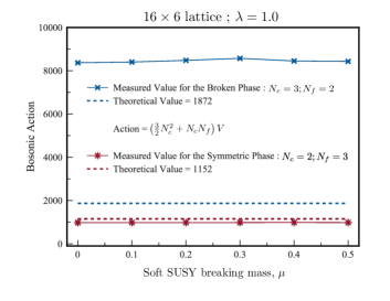
Figure 1: Normalized bosonic action vs soft breaking coupling $\mu$ for $\lambda=1.0$ for a 16x6 lattice

One of clearest signals of supersymmetry breaking can be obtained if one considers the equation of motion for the auxiliary field. We expect the susy preserving case to obey

$$\frac{1}{N_{c}}{\rm Tr\;}\left[\phi(x){\overline{\phi}}(x)\right]=1.$$ (20)

The red points, corresponding to ($N_{f}>N_{c}$) are consistent with this over a wide range of $\mu$. We attribute the small residual deviation as $\mu\to 0$ to our use of antiperiodic boundary conditions which inject explicit ${\cal Q}$ susy breaking into the system. The simulations with $N_{f}<N_{c}$ (blue points) however show a clear signal for spontaneous supersymmetry breaking with the value of this quantity deviating dramatically from its supersymmetric value even as $\mu\to 0$.

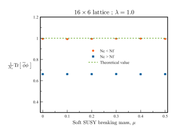
Figure 2: $\frac{1}{N_{c}}{\rm Tr}\phi{\overline{\phi}}$ vs $\mu$ for a ’t Hooft coupling of $\lambda=1.0$ on an 16x6 lattice

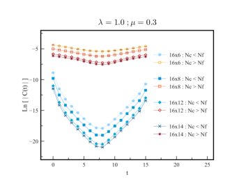
Figure 3: Correlation function C(t) for $\lambda=1.0$ and $\mu=0.3$ on various asymmetric lattices

Finally we turn to our results for a would be Goldstino. We search for this by computing the following two point correlation function

$$C(t)=\sum_{x,y}<O^{\prime}(y,t)O(x,0)>$$ (21)

where $O^{\prime}(y,t)$ and O(x,0) are fermionic operators given by:

$$O(x,0) = \psi_{\mu}(x,0){\cal U}_{\mu}(x,0)\left[\phi(x,0){\overline{\phi}}(x,0)-rI_{N_{c}}\right]$$ (22)

$$O^{\prime}(y,t) = \eta(y,t)\left[\phi(y,t){\overline{\phi}}(y,t)-rI_{N_{c}}\right].$$ (23)

In figure 3 we show the logarithm of this correlator as a function of temporal distance for a range of spatial lattice size, $L=6,8,12$ and 14. The anti-periodic boundary condition is applied along the temporal direction corresponding to T=16 for both $N_{f}>N_{c}$ and $N_{f}<N_{c}$. Clearly a light state with a strong coupling to the would be Goldstino is seen only for the case $N_{f}<N_{c}$.

6 Conclusions

In this talk we describe the construction and simulation of a lattice theory of 2d super QCD with gauge group $U(N_{c})$ and global $U(N_{f})$ flavor symmetry. The model in question possesses ${\cal N}=(2,2)$ supersymmetry in the continuum limit while our lattice formulation preserves a single exact supercharge for non zero lattice spacing. It is expected that the single supersymmetry will be sufficient to ensure that full supersymmetry is regained without fine tuning in the continuum limit. This constitutes the first lattice study of a supersymmetric theory containing fields which transform in both the fundamental and adjoint representations of the gauge group. Our lattice action also contains a ${\cal Q}$-exact Fayet-Iliopoulos term which yields a potential for the scalar fields. We see strong signals that the system is Higgsed and that supersymmetry is spontaneously broken for $N_{f}<N_{c}$ and $r>0$.

The lattice constructions discussed in this paper generalize Joseph:2013jya to three dimensional quiver theories leaving open the possibility of studying 3D super QCD using lattice simulations.

References

- (1) F. Sugino, SuperYang-Mills theories on the two-dimensional lattice with exact supersymmetry, JHEP 0403 (2004) 067, [hep-lat/0401017].
- (2) S. Catterall, A Geometrical approach to N=2 super Yang-Mills theory on the two dimensional lattice, JHEP 0411 (2004) 006, [hep-lat/0410052].
- (3) S. Catterall, D. B. Kaplan, and M. Unsal, Exact lattice supersymmetry, Phys.Rept. 484 (2009) 71–130, [arXiv:0903.4881].
- (4) A. G. Cohen, D. B. Kaplan, E. Katz, and M. Unsal, Supersymmetry on a Euclidean space-time lattice. 1. A Target theory with four supercharges, JHEP 0308 (2003) 024, [hep-lat/0302017].
- (5) A. G. Cohen, D. B. Kaplan, E. Katz, and M. Unsal, Supersymmetry on a Euclidean space-time lattice. 2. Target theories with eight supercharges, JHEP 0312 (2003) 031, [hep-lat/0307012].
- (6) D. B. Kaplan and M. Unsal, A Euclidean lattice construction of supersymmetric Yang-Mills theories with sixteen supercharges, JHEP 0509 (2005) 042, [hep-lat/0503039].
- (7) P. H. Damgaard and S. Matsuura, Classification of supersymmetric lattice gauge theories by orbifolding, JHEP 0707 (2007) 051, [arXiv:0704.2696].
- (8) M. Unsal, Twisted supersymmetric gauge theories and orbifold lattices, JHEP 0610 (2006) 089, [hep-th/0603046].
- (9) S. Catterall, D. Schaich, P. H. Damgaard, T. DeGrand, and J. Giedt, N=4 Supersymmetry on a Space-Time Lattice, Phys.Rev. D90 (2014), no. 6 065013, [arXiv:1405.0644].
- (10) S. Catterall and J. Giedt, Real space renormalization group for twisted lattice =4 super Yang-Mills, JHEP 1411 (2014) 050, [arXiv:1408.7067].
- (11) S. Catterall, P. H. Damgaard, T. Degrand, R. Galvez, and D. Mehta, Phase Structure of Lattice N=4 Super Yang-Mills, JHEP 1211 (2012) 072, [arXiv:1209.5285].
- (12) S. Catterall, E. Dzienkowski, J. Giedt, A. Joseph, and R. Wells, Perturbative renormalization of lattice N=4 super Yang-Mills theory, JHEP 1104 (2011) 074, [arXiv:1102.1725].
- (13) S. Catterall, J. Giedt, and A. Joseph, Twisted supersymmetries in lattice super Yang-Mills theory, JHEP 1310 (2013) 166, [arXiv:1306.3891].
- (14) S. Matsuura, Two-dimensional N=(2,2) Supersymmetric Lattice Gauge Theory with Matter Fields in the Fundamental Representation, JHEP 0807 (2008) 127, [arXiv:0805.4491].
- (15) F. Sugino, Lattice Formulation of Two-Dimensional N=(2,2) SQCD with Exact Supersymmetry, Nucl.Phys. B808 (2009) 292–325, [arXiv:0807.2683].
- (16) S. Catterall, From Twisted Supersymmetry to Orbifold Lattices, JHEP 0801 (2008) 048, [arXiv:0712.2532].
- (17) A. Joseph, Lattice formulation of three-dimensional N=4 gauge theory with fundamental matter fields, JHEP 1309 (2013) 046, [arXiv:1307.3281].