Efficient Reactive Brownian Dynamics

Abstract

We develop a Split Reactive Brownian Dynamics (SRBD) algorithm for particle simulations of reaction-diffusion systems based on the Doi or volume reactivity model, in which pairs of particles react with a specified Poisson rate if they are closer than a chosen reactive distance. In our Doi model, we ensure that the microscopic reaction rules for various association and dissociation reactions are consistent with detailed balance (time reversibility) at thermodynamic equilibrium. The SRBD algorithm uses Strang splitting in time to separate reaction and diffusion, and solves both the diffusion-only and reaction-only subproblems exactly, even at high packing densities. To efficiently process reactions without uncontrolled approximations, SRBD employs an event-driven algorithm that processes reactions in a time-ordered sequence over the duration of the time step. A grid of cells with size larger than all of the reactive distances is used to schedule and process the reactions, but unlike traditional grid-based methods such as Reaction-Diffusion Master Equation (RDME) algorithms, the results of SRBD are statistically independent of the size of the grid used to accelerate the processing of reactions. We use the SRBD algorithm to compute the effective macroscopic reaction rate for both reaction- and diffusion-limited irreversible association in three dimensions, and compare to existing theoretical predictions at low and moderate densities. We also study long-time tails in the time correlation functions for reversible association at thermodynamic equilibrium, and compare to recent theoretical predictions. Finally, we compare different particle and continuum methods on a model exhibiting a Turing-like instability and pattern formation. Our studies reinforce the common finding that microscopic mechanisms and correlations matter for diffusion-limited systems, making continuum and even mesoscopic modeling of such systems difficult or impossible. We also find that for models in which particles diffuse off lattice, such as the Doi model, reactions lead to a spurious enhancement of the effective diffusion coefficients.

I Introduction

It is widely appreciated that fluctuations affect reactive systems in important ways and should be retained, rather than averaged over, in reaction-diffusion modeling. In stochastic biochemical systems, such as reactions inside the cytoplasm, or in catalytic processes, some of the reacting molecules are present in very small numbers and therefore discrete stochastic models are necessary to describe the system BiochemicalDiffusionReaction_Review ; StochChemSpatialNature . In diffusion-limited reactive systems, such as simple coagulation $2A\rightarrow A_{2}$ or annihilation $A+B\rightarrow\emptyset$, spatial fluctuations in the concentration of the reactants grow as the reaction progresses and must be accounted for to accurately model the correct macroscopic behavior Annihilation_AplusB ; Coagulation_Renormalization ; LongTimeTails_ABC ; AsymptoticPowerLaw_ABC . In unstable systems, such as diffusion-driven Turing instabilities Turing_Fluctuations1 ; Turing_Fluctuations2 ; Turing_RDME ; Turing_RDME_2 ; Turing_MD , fluctuations are responsible for initiating the instability and have been shown to profoundly affect the patterns in ways relevant to morphogenesis Turing_Fluctuations1 ; Turing_Fluctuations2 . In systems with a marginally-stable manifold, fluctuations lead to a drift along this manifold that cannot be described by the traditional law of mass action; this has been suggested as being an important mechanism in the emergence of life MarginalStability_Brogioli ; MarginalStability_Brogioli2 ; MarginalStability_LMA .

Much of the work on modeling stochastic chemistry has been for homogeneous, “well-mixed” systems, but there is also a steady and growing interest in spatial models BiochemicalDiffusionReaction_Review ; StochChemSpatialNature ; RDME_Review_Erban . Reaction-diffusion problems are often studied using the Reaction Diffusion Master Equation (RDME) MalekRDME1975 ; KeizerBook ; GardinerBook ; vanKampen:07 , which extends the well-known Chemical Master Equation (CME) to spatially-varying systems. In the RDME, the system is subdivided into reactive subvolumes (cells) and diffusion is modeled as a discrete random walk by particles hopping between cells, while reactions are modeled using CMEs local to each cell RDME_Review_Erban . A large number of efficient and elaborate event-driven kinetic Monte Carlo algorithms for solving the CME and RDME, exactly or approximately, have been developed with many tracing their origins to the Stochastic Simulation Algorithm (SSA) of Gillespie GillespieSSAreview . Of particular importance to the work presented here is the next subvolume method NextSubvolumeMethod_MesoRD , which is an event-driven algorithm in which each cell independently schedules the next reactive or diffusive event to take place inside it. There are also a number of approximate techniques that speed the Monte Carlo simulation of the RDME when there are many particles per reactive cell, i.e., when the fluctuations are relatively weak. For example, in multinomial diffusion algorithms MultinomialDiffusion_Gillespie ; MultinomialDiffusion the diffusive hops between reactive cells are simulated by sampling the number of jumps between neighboring cells using a multinomial distribution. This can be combined with tau leaping for the reactions using time splitting, as summarized in Appendix A in FluctReactDiff , to give a method that does not simulate each individual event. One can take this one step further toward the continuum limit by switching to a real number rather than an integer representation for the number of molecules in each cell, and use fluctuating hydrodynamics to simulate diffusion FluctReactDiff , giving a method that scales efficiently to the deterministic reaction-diffusion limit.

The RDME, and related approaches based on local reactions inside each reactive cell, have a number of important drawbacks, such as the lack of convergence as the RDME grid is refined in the presence of binary reactions MesoRD_GridResolution ; RDME_Bimolecular_Petzold ; CRDME . This means that one must choose the cells to be not too large, so that spatial variations are resolved, nor too small, so that binary reactions do not disappear. In fact, the common justification for the RDME is to assume that each cell is well-mixed and homogeneous GillespieSSAreview , which is not true if one makes the cells too small or too large. Variants of the RDME have been proposed that improve or eliminate the lack of convergence as the grid is refined, the most relevant to this work being the convergent RDME (CRDME) of Isaacson CRDME , in which reactions can happen between molecules in neighboring cells as well. Another drawback of the RDME is the fact that the CME, and therefore the RDME, require as input the macroscopic or mesoscopic rates that enter in the law of mass action, rather than microscopic rates that define the reaction-diffusion process. The conversion from the microscopic to the macroscopic rates is nontrivial even for systems with only a single reaction, and even at very low densities ReactionDiffusion_Doi ; DoiModel_Erban , let alone at finite densities Coagulation_Renormalization_PRL ; Coagulation_Renormalization or for systems with many species and reactions. It is not correct, in general, to use the macroscopic law of mass action coefficients in the RDME, since this double counts fluctuations, as it is well-known that the reaction rates are renormalized by spatial fluctuations Coagulation_Renormalization_PRL ; Coagulation_Renormalization ; RenormalizationReactionDiffusion_Review . The conversion of microscopic to mesoscopic rates, i.e., rates that depend on the cell size, is to our knowledge a completely open problem. As clearly shown by the calculations of Erban and Chapman DoiModel_Erban , one can, alternatively, think of the RDME as a microscopic (rather than a mesoscopic or coarse-grained) model if the cell size is comparable to the reaction radius, as is rather common in physics where this is usually simply referred to as a “lattice model” of reaction-diffusion RenormalizationReactionDiffusion_Review . But when the cells are microscopic in size, the RDME suffers from large grid artifacts such as dependence on the exact shape of the cells and broken translational and rotational invariance.

An alternative approach, which removes all of the aforementioned drawbacks, is to use a particle model of reaction-diffusion systems. The main drawback of particle methods, which we address in this work, is their inefficiency relative to RDME-like coarse-grained descriptions. In particle-based models, molecules of each reactive species are tracked explicitly, and can appear, disappear or change species via reactions. This leads to a grid-free method that takes as input well-defined microscopic rates. Particle-based reaction-diffusion models are a combination of two models, a model of diffusion and a model of reaction. A typical diffusion model employed in biochemical modeling is that the individual particles diffuse as uncorrelated Brownian walkers, with each species $k$ having a specified diffusion coefficient $D_{k}$. While this model is not easily justified in either gases or liquids, it is commonly used and we will adopt it in this work, postponing further discussion to the Conclusions. There are three commonly-used reactive models, which we explain on the binary reaction $A+B\rightarrow C$ involving two reacting particles of species $A$ and $B$. Note that reactions involving more than two particles are microscopically extremely improbable and do not need to be considered. In the surface reactivity or Smoluchowski model, two particles of species $A$ and $B$ react as soon as they approach closer than a distance $R_{AB}$, which defines the reactive radius for a particular reaction. As explained in detail in the Introduction of DoiModel_Erban , matching this kind of microscopic reaction model to measured macroscopic reaction rates typically requires reaction radii that are too small; using a reactive radius comparable to the expected steric exclusion between molecules leads to a notable over-estimation of the reaction rate. Furthermore, the Smoluchowski model is difficult to make consistent with detailed balance (and thus all of equilibrium statistical mechanics) for reversible reactions. This is because microscopic reversibility requires that the reverse reaction $C\rightarrow A+B$ place the products at a distance exactly equal to $R_{AB}$, which would lead to their immediate reaction. One way to resolve this problem is to allow some contacts between particles $A$ and $B$ to be non-reactive, i.e., to replace the fully absorbing boundary conditions in the Smoluchowski model with partial absorption Robin boundaries, as proposed by Collins and Kimball DiffusionControlled_RobinBC , and studied in more detail and employed in simulations in a number of subsequent papers CollinsKimball_1 ; CollinsKimball_2 ; CollinsKimball_3 ; CollinsKimball_4 .

The volume reactivity or Doi model ReactionDiffusion_Doi ; DoiModel_Erban corrects the shortcomings of the surface reactivity models. Somewhat ironically, the model was proposed by Doi in his seminal work ReactionDiffusion_Doi only as a way to study the Smoluchowski model in a mathematically simpler way; recently Erban and Chapman DoiModel_Erban suggested that this model has a lot of merit on its own right. We employ the Doi model in this work and therefore it is important to formulate it precisely. In this model, all pairs of particles of species $A$ and $B$ that are closer than the reactive radius $R_{AB}$ can react with one another as a Poisson process of rate $\lambda$, that is, the probability that a pair of particles for which $r_{AB}\leq R_{AB}$ react during an infinitesimal time interval $dt$ is $\lambda\,dt$ . Since this model takes as input two rather than one parameter, one can adjust them independently to model experimental systems more realistically. Notably, the reactive radius can be chosen to have a realistic value corresponding to the physical size of the reacting molecules, and the reaction rate $\lambda$ can be tuned to reproduce measured macroscopic rates. Nevertheless, we admit that in practical applications the Doi model itself is a rather crude approximation of the actual molecular structure and reaction mechanisms, and it may be difficult to define precisely and measure accurately anything other than some effective macroscopic reaction rates. As we explain in more detail later, achieving microscopic reversibility (detailed balance) is quite straightforward in the Doi model. Furthermore, while the Smoluchowski model is inherently diffusion-limited, the Doi model can be used to study either reaction-limited ($\lambda$ small) or diffusion-limited systems ($\lambda$ large). In the limit of infinitely fast reactions, $\lambda\rightarrow\infty$, the Doi model becomes equivalent to the Smoluchowski model, whereas in the limit $\lambda\rightarrow 0$ one obtains a well-mixed model.

There are a number of existing particle-based algorithms for simulating reaction-diffusion systems. For the Smoluchowski model, an exact and efficient algorithm is the First Passage Kinetic Monte Carlo (FPKMC), first proposed by Oppelstrup et al. in FPKMC_PRL and then extended and improved in FPKMC1 ; FPKMC2 ; FPKMC_drift , and generalized to lattice models in FPKMC_lattice . The event-driven FPKMC algorithm is a combination of two key ideas: solving pair problems analytically as in the Green’s Function Reaction Dynamics (GFRD) GFRD ; GFRD_KMC , and using protective domains to ensure an exact breakdown of the multibody problem into pairwise problems , as in diffusion Monte Carlo methods used in quantum mechanics KLV_PRE . The FPKMC algorithm can, in principle, be generalized to the Doi model, but not without sacrificing its exactness. Namely, while for the Smoluchowski model the multibody reactive hard-sphere problem can always be broken into two-body problems, in the Doi model three or more particles can be within a reactive distance. However, FPKMC is not efficient at higher density, where it becomes more and more difficult to break the multibody problem into few-body problems. For these reasons, we pursue a different approach in this work, which is most efficient at higher densities and is rather straightforward to implement compared to FPKMC.

Prior approaches to simulating the Doi model have been based on time splitting between diffusion and reaction. Detailed algorithmic descriptions are missing in prior work, but the basic idea is as follows. Given a time step size $\Delta t$, the particles are first diffused over the time interval $\Delta t$, and then reactions are processed between pairs of particles within the reactive radius; this is similar to what is done in a number of popular software packages for particle modeling of reaction-diffusion such as Smoldyn Smoldyn_v2 and MesoRD MesoRD . Two main factors make such particle methods inefficient. The first one is the use of hopping in small intervals $\Delta t$ to bring particles to react; this is completely bypassed by the FPKMC method FPKMC_PRL at the expense of algorithmic complexity. The second factor is that at every time step, one must do neighbor searches in order to identify pairs of particles that may react during the time step. This is a necessary cost when reaction-diffusion is combined with molecular dynamics BD_MD_ReaDDy , but, as we show here, is a superfluous cost when simulating simple reaction-diffusion processes. Furthermore, even with the expensive neighbor searches performed, the algorithm used by Robinson et al. DoiNumerics_Erban employs some approximations when processing reactions, which can introduce uncontrolled bias. For example, the reactions are processed in turn in the same order, and it is assumed that the probability of reaction during the time interval is small, $\lambda\,\Delta t\ll 1$.

In this paper, we develop Split Reactive Brownian Dynamics (SRBD) as an efficient algorithm for simulating the Doi model with controlled accuracy. Our algorithm still uses time splitting between diffusion and reaction, and therefore, will be less efficient at low densities. However, unlike existing methods, it bypasses the need to find pairs of nearby particles at each time step. In this sense, SRBD gains efficiency not by increasing $\Delta t$ as FPKMC does, but rather, by reducing the cost of one time step. Notably, if the reaction rate is small and reactions are infrequent, the algorithm adds a minimal cost per time step for processing the reactions, on top of the cost of diffusing the particles. If the reaction rate is large and a particle can undergo more than one reaction per time step, the algorithm correctly accounts for this. The only error introduced is the splitting error, and therefore the error can be controlled easily by reducing the time step so that particles diffuse only a fraction of the reactive radius per time step.

In Section II we present the microscopic reactive model used in SRBD, along with algorithmic details of how diffusion and reaction are handled in the SRBD time stepping scheme. In Section III, we use the SRBD algorithm to study the differences between reaction-limited and diffusion-limited regimes for irreversible dissociation, reversible association, and a pattern-forming system. We offer some conclusions and a discussion of open problems in Section IV.

II Stochastic Reactive Brownian Dynamics

In SRBD, we cover the domain with a regular grid of cells. However, unlike the reactive cells in RDME, and like cells used in other particle algorithms such as molecular dynamics, in SRBD the cells are only used to help efficiently identify pairs of particles that are closer than their reactive distance, and the size of the cells only affects the computational efficiency but does not affect the results. We denote the largest reactive distance among all possible binary reactions with $R_{\max}$. The only condition on the cell size in SRBD is that all cells must be larger than $R_{\max}$ in each dimension. This ensures that only particles that are in neighboring cells (we count a given cell as a neighbor of itself) can be within a reactive distance of one another. If the set of possible reactions changes with time and at some point $R_{\max}$ exceeds the current cell size, one can simply re-generates the grid of cells at the beginning of the next time step.

The SRBD algorithm itself is a combination of the key ideas behind two existing methods. The first one is the next subvolume method NextSubvolumeMethod_MesoRD for solving the RDME exactly, and the second one is the Isotropic Direct Simulation Monte Carlo (I-DSMC) method for simulating a stochastic hard sphere dynamics model of a fluid SHSD_PRL ; SHSD . Unlike the next subvolume method, which treats diffusion using a master equation as just one more reactive channel, we treat diffusion separately from reaction. This allows one to substitute the “motion module” from simple diffusion of uncorrelated walkers to something more realistic, such as hydrodynamically correlated walkers DiffusionJSTAT . Following the diffusive propagation of the particles, we process reactions between reactive pairs using an exact event-driven algorithm in which reactions are scheduled in an event queue and processed one by one. As in the next subvolume method, reactive events are scheduled per cell rather than per particle as in FPKMC. As in the I-DSMC method (and also the CRDME method), reactions can take place between molecules in two disjoint neighboring cells, using rejection to correct for the fact that pairs of particles chosen to react may not actually be within the reactive distance.

In this section we give a complete description of the SRBD algorithm, as implemented in Fortran in a code that is available freely at https://github.com/stochasticHydroTools/SRBD. We assume periodic boundary conditions throughout this paper. We will focus the algorithmic description on the handling of binary reactions involving two species, $A+B\rightarrow\dots$, or involving the same species $A+A\rightarrow\dots$. However, it should be clear that the algorithm can be trivially generalized to handle reaction networks containing many competing reaction channels and many species (as done in our code).

For comparison, in our code and in the results reported here, we have also studied a method in which the diffusion model is the same as in SRBD (independent Brownian walkers), but the reactions are performed using a grid of cells as in the RDME. The difference with the RDME is that the particles diffuse via a continuous random walk instead of a jump process. This kind of model was proposed and studied in BD_RDME , and an algorithm was developed based on time splitting of reaction and diffusion. We modify the method described in BD_RDME in order to improve translational (Galilean) invariance. Namely, before performing reactions, we randomly shift the grid of reactive cells by an amount uniformly distributed in $[-h/2,h/2)$, where $h$ is the grid spacing, along each dimension. This is commonly done in a number of other particle methods MPCD_Review in periodic domains. We will refer to this approach as Split Brownian Dynamics with Reaction Master Equation (S-BD-RME). In S-BD-RME, we employ the same microscopic reaction rules given in Section II.1.1 for SRBD, replacing “within distance $R$” by “in the same reactive cell,” and replacing “uniformly in a sphere centered at the $A$ with radius $R$” with “in the same reactive cell”. This makes all reactions in S-BD-RME local to a reactive cell, making it possible to parallelize the algorithm straightforwardly.

Also for comparison, we will include in a number of our tests the traditional RDME approach. We solve the RDME not by using the expensive next reaction method, but rather, by using an efficient (easily parallelizable) but approximate algorithm described in detail in Appendix A in FluctReactDiff . This algorithm is based on time splitting of diffusion and reaction and treating diffusion using the multinomial diffusion algorithm proposed in MultinomialDiffusion ; the only source of error in this algorithm is the finite size of the time step size $\Delta t$, and we have confirmed that reducing $\Delta t$ in half does not statistically change the results reported here. One can use the S-BD-RME algorithm to simulate the RDME simply by replacing the continuous random walks by discrete jumping on a lattice, and not performing random grid shifts. However, this defeats the key efficiency of the RDME over particle methods, namely, that one does not have to track individual particles. Instead, in the RDME one only keeps track of the total number of particles of each species in each reactive cell. This can be a great saving if there are many particles per cell, but will be less efficient than particle tracking if there are on average fewer than one molecule per reactive cell.

II.1 Microscopic Model

We denote the time-dependent positions of particle $i$ with species $s(i)$ by $\boldsymbol{q}_{i}\left(t\right)\in\mathbb{R}^{d}$, where the dimension $d$ is a small integer (typically 1, 2 or 3), and $i=1,\dots,N_{p}$, where $N_{p}(t)$ is the total number of particles at time $t$. As explained in the Introduction, in this work we use the simplest model of diffusion: each particle is treated as a sphere with only translational degrees of freedom and diffuses as a Brownian walker (i.e., performs a continuous random walk) independently of any other particles. We assume that all particles of species $k$ diffuse with the same coefficient $D_{k}$, $k=1,\dots,N_{s}$. As also explained in the Introduction, we use the Doi model DoiModel_Erban for binary reactions: each pair of particles of species $A$ and $B$ (respectively, $A)$ that are closer than the reactive radius $R_{AB}$ (respectively, $R_{AA}$) can react with one another as a Poisson process of rate $\lambda$. Different reactions $r$, $r=1,\dots,N_{r}$, have different rates $\lambda_{r}$ (with units of inverse time) specified as input parameters. In this work we assume an additive hard-sphere model,

$$R_{AB}=R_{A}+R_{B},\quad\mbox{ and similarly,}\quad R_{AA}=2R_{A},$$

where the radius $R_{k}$ of particles of species $k$ is an input parameter. This can easily be relaxed, and a different reaction distance can be specified for each binary reaction.

A proper microscopic reaction model requires complete specification of what happens when a chemical reaction occurs. Specifically, it requires one to specify which reactant particles change species or disappear, and which product particles are created and where. We have constructed a list of microscopic reactive rules implemented in our code by following the principle of microscopic reversibility or detailed balance. We explain this in some detail because of its importance to having a reaction-diffusion model consistent with equilibrium thermodynamics and statistical mechanics DiffusionLimited_NonDB , which we believe to be of utmost importance. To our knowledge, few prior works have paid close attention to this condition; for example, the Doi model of a reversible reaction $A+B\leftrightarrow C$ proposed in DoiModel_Reversible_Erban is not consistent with detailed balance.

II.1.1 Detailed Balance

We postulate, consistent with a long tradition of works in statistical mechanics KeizerBook ; GardinerBook ; vanKampen:07 , that chemical reactions do not alter the state of thermodynamic equilibrium. Instead, the state of thermodynamic equilibrium is set by chemical potentials only. For an ideal solution/gas of non-interacting particles, the desired equilibrium distribution is given by a product Poisson measure, i.e., the probability of finding any given molecule (particle) is uniform over the domain and independent of other molecules. The principle of detailed balance then requires that, starting from a configuration sampled from the equilibrium state, the probability of observing a forward reaction is equal to that of the reverse reaction. That is, the reaction-diffusion Markov process should be time reversible with respect to an equilibrium distribution given by a product Poisson invariant measure .

Satisfying detailed balance with respect to such a simple equilibrium measure is straightforward and simply requires making each reverse reaction be the microscopic reverse of the corresponding forward reaction. For each forward reaction, we define a specific mechanism that we believe is physically sensible, but note that this choice is not unique. However, once the forward mechanism is chosen the reverse mechanism is uniquely determined by detailed balance. We summarize the forward/reverse reaction rules we have used in our code in Appendix A.

It is important to note that we do not require that each reaction be reversible nor do we require the existence of a thermodynamic equilibrium. Our method can be used without difficulty to model systems that never reach equilibrium or violate detailed balance. For example, for a reaction $A\rightarrow B+C$, one can treat the maximum possible distance between the product particles $R_{BC}$ as an input parameter (unbinding radius) potentially different from the Doi reactive radius (binding radius) for the reverse reaction. However, by adopting microscopically reversible reaction rules we guarantee that if all reactions are reversible (with the same binding and unbinding radius), there exists a unique state of thermodynamic equilibrium given by a uniform product Poisson measure; furthermore, the equilibrium dynamics will be time reversible. This makes our model fully consistent with the fundamental principles of equilibrium statistical mechanics; for example, as we show in Section III.3, the equilibrium constants (concentrations) will be independent of kinetics (rates).

II.1.2 Enhancement of diffusion coefficients by reaction

It is important here to point out a somewhat unphysical consequence of the microscopic Doi reaction model for reversible reactions: increased species diffusion due to reactions. For specificity, let us consider the reversible reaction $A+B\leftrightarrow C$ and denote the number densities of the reactants with $\boldsymbol{n}=\left(n_{A},n_{B},n_{C}\right)$. In the RDME model, reacting particles have effectively the same position, since they need to be on the same lattice site to react. Similarly, the reverse reaction creates particles at the same site. This implies that if one constructs, for example, the linear combination $\tilde{n}=n_{A}+n_{B}+2n_{C}$, the reaction strictly preserves $\tilde{n}$ locally. This means that $\tilde{n}$ evolves by diffusion only.

In the SRBD or S-BD-RME models, however, the positions of the reacting particles are off lattice. This means that, even in the absence of explicit particle diffusion, the quantity $\tilde{n}$ will evolve due to reactions. In particular, assume that an $A$ and a $B$ particle react and the $B$ becomes a $C$, and thereafter the $C$ decays via the reverse reaction into a $B$ and creates an $A$ within a reactive radius of the original $B$. This net consequence of this sequence of successive forward and reverse reactions is that the $A$ particle has randomly displaced, from one position inside a reactive sphere centered at the $B$ particle, to a new position within this sphere. This is an effective diffusive jump of the $A$ particle and leads to an enhancement of the diffusion coefficient of the quantity $\tilde{n}$ on the order of $R_{AB}^{2}/\tau$, where $\tau$ is a reactive time for the sequence $A+B\rightarrow C\rightarrow A+B$. This effective enhancement can become important when $R_{AB}$ is large, and lead to different physical behavior between the RDME and the SRBD or S-BD-RME models, as we will demonstrate explicitly in Sections III.3 and III.4, and discuss further in the Conclusions.

II.2 Time Splitting

The only approximation we make in our SRBD algorithm is that diffusion and reaction are handled separately by using time splitting. We use the well-known second-order Strang splitting method, and then solve the diffusion and reaction subproblems exactly. Specifically, one time step of duration $\Delta t$ going from time level $n$ to $n+1$ is performed as described in Algorithm 1. The errors induced in expectation values (observables) by the Strang splitting are of order $O\left(\Delta t^{2}\right)$.

1. Diffuse all particles $i$ present at time $t^{n}$ for half a time step

   $$\boldsymbol{q}_{i}^{n+\frac{1}{2}}=\boldsymbol{q}_{i}^{n}+\sqrt{D_{s(i)}\Delta t}\,\boldsymbol{\mathcal{N}}\left(0,1\right),$$

   where $\boldsymbol{\mathcal{N}}\left(0,1\right)$ denotes a Gaussian random variate of mean zero and unit variance, sampled independently for each particle and at each time step.

2. Process reactions exactly over a time interval $\Delta t$ during which the particles do not diffuse (i.e., they stay in place) using Algorithm 2. If using S-BD-RME, choose a grid of cells to perform the reactions in, potentially randomly shifted from a reference grid to improve translational invariance, and then process reactions in each cell independently using the traditional SSA algorithm.

3. Diffuse all remaining and newly-created particles $i$ for half a time step

   $$\boldsymbol{q}_{i}^{n+1}=\boldsymbol{q}_{i}^{n+\frac{1}{2}}+\sqrt{D_{s(i)}\Delta t}\,\boldsymbol{\mathcal{N}}\left(0,1\right).$$

Algorithm 1 Split time step of the SRBD or S-BD-RME algorithms.

II.3 Processing Reactions in SRBD

We now turn our attention to the core of the SRBD algorithm, processing reactions over a time interval $\Delta t$ during which the particles do not diffuse. We perform this reaction-only step exactly, i.e., we sample from the correct Markov process without any approximations. We focus here on processing binary reactions since reactions involving zero or one reactants are trivial to handle.

A naive algorithm would proceed as follows. First, for each binary reaction, create a list of all pairs of particles that could react because they are within a reactive distance of each other (note that one pair can in principle participate in a number of different reactions). Let the number of potential pairs for reaction $r$ be $N_{pr}$. Set the propensity (rate) for reaction $r$ to $N_{pr}\lambda_{r}$, and select the next reaction to happen and increment the time counter (if less than $\Delta t$) using the traditional SSA algorithm. Once a specific reaction is selected, select one of the $N_{pr}$ pairs for that reaction uniformly at random, and process the reaction using the microscopic reaction rules described in Appendix A. Update the list of pairs and repeat the process until a time $\Delta t$ has elapsed. This algorithm, while clearly correct, is very inefficient due to the need to search for pairs of overlapping particles at each step, and to update this list after each reaction is processed. In Algorithm 2 we summarize an algorithm that is identical in law. In other words, the algorithm selects pairs of particles with the correct probability rates, without ever explicitly searching for pairs within a reactive distance. We detail the various steps in subsequent sections.

Note that the algorithm presented here requires having efficient dynamic spatial data structures that enable finding all particles that are in a given cell, as well as keeping an accurate count of the number of particles of each species in each cell. The most efficient, in both storage and time, and simplest data structure that can be used for this purpose is what we will refer to as linked-list cells (LLCs) AED_Review . These are essentially integer-based linked lists, one list for each cell and each species, that stores an integer identifier for all particles of the given species in the given cell, see the book Allen_Tildesley_book for implementation details. Additionally, one requires a data structure for managing the event queue; our implementation uses a heap of fixed size equal to the number of cells for this purpose.

1. Prepare: Build linked-list cells (LLCs) and reset the event queue.

2. Sample the time to the next reaction for each cell $i$ (see Algorithm 3) $\delta t_{i}$ and compute the scheduled next reaction time $t_{i}=t+\delta t_{i}$. If the scheduled time $t_{i}\leq t^{n}+\Delta t$, insert the scheduled reaction event into the event queue with time stamp $t_{i}$.

3. Event loop: Until the event queue is empty, do:

   1. Select cell $i$ on top of the queue with time stamp $t_{i}$, $t^{n}\leq t_{i}\leq t^{n}+\Delta t$, and advance the global time to $t=t_{i}$.

   2. Select next reaction to happen in cell $i$ using a traditional KMC/SSA method.

   3. If the reaction is unary, select a particle in cell $i$ to undergo the chosen reaction. If the reaction is binary, select a pair of particles, one in cell $i$ and the other in one of its neighboring cells, to undergo the chosen reaction. For binary reactions, if particles do not overlap, i.e., they are not within a reactive radius of each other, then skip to step 3e.

   4. Process the reaction (see Algorithm 4), creating/destroying particles and updating the LLCs as necessary.

   5. For each cell $j$ that is a neighbor of cell $i$ (including cell $i$) that was (potentially) affected by the reaction, reschedule the time to the next reaction $\delta t_{j}$ (see Algorithm 3). If $t_{j}=t+\delta t_{j}<t+\Delta t$ schedule the next event for cell $j$ at time $t_{j}$ and update the event queue, otherwise delete cell $j$ from the queue.

Algorithm 2 Summary of the SRBD reaction step 2 in Algorithm 1 during the $n$-th time step.

II.3.1 Scheduling reactions

For unary reactions such as decay $A\rightarrow\dots$, what we mean by a reaction occurring in cell $i$ is that the particle undergoing the reaction is in cell $i$. For binary hetero-reactions with different reactants $A+B\rightarrow...$ with Doi rate $\lambda$, we schedule separately the two ordered reactions $A+B\rightarrow...$ and $B+A\rightarrow...$, i.e., we distinguish one of the two particles as the “first” particle and the other as the “second” particle. Each of these two reactions occurs with half the rate of the original (unordered) reaction. We associate a given binary reaction to the cell in which the first particle is located. For binary reactions with a single species, $A+A\rightarrow\dots$, we also order the two reacting particles into a first and a second particle, and associate the reaction with the cell of the first particle. The effective rate of the ordered reactions is again half of the original rate because each pair is scheduled for reaction twice. A little thought reveals that no special treatment is needed for a homo-reaction $A+A\rightarrow\dots$, where both of the particles are in the same cell except for rejecting self-reactions; each pair of particles can again be selected twice.

Scheduling the time $\delta t$ until the next reaction to occur in a given cell is done by computing the total reaction rate (called propensity in the SSA literature) $\alpha$ over all reactions associated with that cell, and sampling an exponentially-distributed time lag $\delta t$ with mean $\alpha^{-1}$, as detailed in Algorithm 3. Note that the computation in Algorithm 3 over-estimates the actual rate for binary reactions since it does not account for whether the particles actually overlap; we correct for this using rejection. Specifically, if a pair selected to react does not overlap, we reject the pair. Similarly, for homo-reactions $A+A\rightarrow\dots$ we correct for the fact that we compute the number of pairs of particles of species $A$ as $N_{A}^{2}/2$ instead of $N_{A}\left(N_{A}-1\right)/2$ by rejecting reactions of a particle with itself.

• For each binary reaction $r$ for cell $i$, $A+B\rightarrow...$ where we allow for the possibility that $B=A$ and the order of the reactants matters if $B\neq A$, compute the rate in cell $i$ as

  $$\alpha_{r}=\frac{\lambda}{2}N_{A}N_{B}^{\prime}$$

  where $N_{A}$ is the number of $A$ particles in cell $i$, and $N_{B}^{\prime}$ is the total number of $B$ particles in the neighborhood of $i$.

• Add the rates of all possible reactions, $\alpha=\sum_{r=1}^{N_{r}}\alpha_{r}$ (as in ordinary SSA).

• Sample an exponentially distributed random number $\delta t_{i}$ with mean $\alpha^{-1}$.

Algorithm 3 Algorithm used to schedule the time to the next reaction $\delta t_{i}$ for cell $i$ during steps 2 and 3e in Algorithm 2.

II.3.2 Processing binary reactions

Once a given cell is chosen to have a reaction occur in it, one must select one (for unary reactions) or two (for binary reactions) particles to participate in the reaction, randomly and uniformly from among all particles of the required species that are in the given cell or one of its neighboring cells. This step is made efficient by using LLCs and the counts of the number of particles of each species in each cell. We give additional details of the processing of binary reactions in Algorithm 4.

• Randomly and uniformly select a particle of species $A$ that is in cell $i$, and another particle of species $B$ from a cell $j$ that neighbors cell $i$. Note that this can select the same particle twice if $B=A$; when this happens, skip the remaining steps.

• Test if the two particles are within their reactive distance, and if not, skip the remaining steps.

• Otherwise, process the reaction by deleting and adding particles depending on the reaction products, following the microscopic reaction rules explained in Appendix A. While processing the reactions, keep the LLCs up to date and keep track of whether any reaction changes the population of cell $i$ (number of particles of each species in that cell), and also whether the population of cell $j$ changes.

• Reschedule the time to the next reaction $\delta t_{i}$ for cell $i$ using Algorithm 3. If $t_{i}=t+\delta t_{i}<t+\Delta t$ schedule the next event for cell $i$ at time $t_{i}$ and update the event queue, otherwise delete cell $i$ from the queue.

• If the population of cell $i$ changed, update the event prediction for all neighbor cells of $i$.

• If the population of cell $j$ changed, update the event prediction for all cell neighbors of $j$ that are not also neighbors of $i$.

Algorithm 4 Algorithm used in steps 3d and 3e of Algorithm 2 to process a binary reaction $A+B\rightarrow\dots$ (where it may be that $B=A$) associated with cell $i$ at global time $t$.

III Examples

In this section we apply the SRBD algorithm to a number of reaction-diffusion problems, and compare the numerical results to theoretical predictions and results obtained using RDME, as well as S-BD-RME. First, in Section III.1, we explore the relationship between microscopic reaction rates and the effective macroscopic rates for reaction- and especially diffusion-limited irreversible bimolecular reactions in three dimensions. In Section III.2 we briefly discuss how the choice of the grid cell size in the SRBD algorithm affects the computational efficiency of the algorithm. In Section III.3 we study the dynamics of concentration fluctuations at thermodynamic equilibrium for diffusion-limited reversible association in two dimensions. Lastly, in Section III.4 we study the formation of Turing-like patterns in a reaction-limited two-dimensional system.

III.1 Conversion from microscopic to macroscopic reaction rates

One of the key issues when comparing different methods, such as SRBD and RDME, is ensuring that the parameters in the two models are both consistent with the same effective macroscopic model at length scales much larger than the discretization scale (i.e., reactive distances in SRBD or grid size in RDME), and time scales much larger than the microscopic ones. This is especially difficult to do because the effective macroscopic model is non-trivial to obtain for reaction-diffusion problems, and is not always given by a simple deterministic reaction-diffusion partial differential equation. In particular, a large body of literature has emerged over the past several decades showing that the macroscopic behavior is unusual for diffusion-limited systems, i.e., systems in which reactions happen quickly once reactants find each other in physical proximity AsymptoticPowerLaw_ABC ; LongTimeTails_ABC ; RelaxationTime_ABC ; Coagulation_Renormalization ; Coagulation_Renormalization_PRL ; DiffusionLimited_NonDB ; DiffusionLimitedAnnihilation . For example, the traditional law of mass action is known to break down in simple diffusion-limited coagulation even in three dimensions Coagulation_Renormalization ; Coagulation_Renormalization_PRL , making it impossible to even define what is meant by an effective or macroscopic reaction rate. Even when the law of mass action is formally recovered for the instantaneous reaction rate, long-term memory effects appear in the long-time dynamics AsymptoticPowerLaw_ABC ; LongTimeTails_ABC . In general, in diffusion-limited systems nontrivial correlations between fluctuations of the number densities of different species appear at molecular scales, and diffusion coefficients enter in the macroscopic “reaction rates” in addition to the microscopic reaction rates. This is to be contrasted with the much simpler behavior for reaction-limited systems, where diffusion dominates and uniformly mixes the reactants, thus eliminating microscopic spatial correlations between different species.

To illustrate these subtle physical effects and confirm that the SRBD model and algorithm produce the correct results both in reaction-limited and diffusion-limited settings, we study here two simple examples for which analytical predictions are available. The first is a one-species model of coagulation, $A+A\rightarrow A$, and the second one is a two-species model of annihilation, $A+B\rightarrow B$, both of which we study in three dimensions. We define an effective macroscopic binary reaction rate $k$ as follows. We insert particles of species $A$ randomly and uniformly into the system via the reaction $\emptyset\underset{k_{i}}{\rightarrow}A$, and wait until a steady state is established at a given average (over space and time) number density $n_{A}$. The effective forward rate for the binary reaction at the steady state number density (observe that the average number density of $B$ molecules is unchanged by the reaction $A+B\rightarrow B$) is then defined as $k=k_{i}/\left(n_{A}n_{B}\right)$ for $A+B\rightarrow B$, and $k=k_{i}/n_{A}^{2}$ for $A+A\rightarrow A$.

III.1.1 Reaction-Limited versus Diffusion-Limited Rates

For sufficiently low packing densities $\phi$ (defined precisely later), one can estimate the effective (macroscopic) association or forward reaction rate $k_{0}=\lim_{\phi\rightarrow 0^{+}}k$ for binary reactions in SRBD by generalizing the approach originally proposed by Smoluchowski for the Doi reactivity model. In this approach, many-body effects are neglected, as later justified by Doi ReactionDiffusion_Doi . Details can be found in the work of Erban and Chapman DoiModel_Erban ; here we summarize the important results. For a single reaction $A+B\rightarrow\dots$ or $A+A\rightarrow\dots$ in three dimensions, at low densities, the macroscopic reaction rate $k_{0}$ (units $\text{m}^{3}/\text{s}$) is predicted to be related to the microscopic rate $\lambda$ (units $\text{s}^{-1})$ and the reactive radius $R$ in the Doi model via DoiModel_Erban

$$k_{0}=s\left(4\pi DR\right)\left[1-\sqrt{\frac{D}{\lambda R^{2}}}\;\tanh\left(\sqrt{\frac{\lambda R^{2}}{D}}\right)\right],$$ (1)

where $s=1$, $D=D_{AB}=D_{A}+D_{B}$ and $R=R_{AB}=R_{A}+R_{B}$ for $A+B\rightarrow\dots$, and $s=1/2$, $D=2D_{A}$ and $R=R_{AA}=2R_{A}$ for $A+A\rightarrow\dots$.

Let us define a dimensionless number

$$r=\frac{\lambda R^{2}}{D},$$

which compares the reaction rate to the diffusion rate. First, note that for all values of $r$ we have $k_{0}<4\pi DR$. If $r\gg 1$, the system is diffusion-limited, and $k_{0}\approx k_{S}^{\text{SRBD}}$ approaches the Smoluchowski rate $k_{S}^{\text{SRBD}}=4\pi DR$, i.e., the rate that would be obtained if particles reacted upon first touching. For $r\ll 1$, the system is reaction-limited, and we obtain

$$k_{0}\approx k_{\text{mix}}=s\frac{4\pi}{3}R^{3}\lambda.$$ (2)

This result has a very simple physical interpretation. In the limit $r\ll 1$, the particle positions are uncorrelated, i.e., the system is “uniformly mixed” at microscopic scales. Therefore, to find the instantaneous reaction rate one can simply multiply by $\lambda$ the total number of overlapping particle pairs $V_{r}n_{A}n_{B}$ (taking $n_{B}\equiv n_{A}$ for the one-species case), where $V_{r}=4\pi R^{3}/3$ is the reactive volume, which gives the total reaction rate as $k_{0}n_{A}n_{B}\approx\lambda V_{r}n_{A}n_{B}.$ The formula (2), unlike (1), applies at all densities, i.e., $k\approx k_{0}$ independent of the density for reaction-limited systems. Furthermore, while it is not possible to generalize (1) to two dimensions, there is no problem in generalizing (2) to any dimension, simply by using the corresponding formula for the volume of the reactive sphere $V_{r}$. Lastly, while (1) does not generalize to the case of many species and reactions, (2) continues to apply for each reaction in reaction-limited systems. This emphasizes the fact that reaction-limited systems are much simpler to model than diffusion-limited ones. We will use this in Section III.4 when studying Turing-like pattern formation in a reaction-limited system.

One can argue that, in general, if a system is well described by (deterministic or fluctuating) hydrodynamics, it should be in the reaction-limited regime unless the reactants are very dilute. For a generic binary reaction $A+B\rightarrow\dots$, an important characteristic length scale is the so-called penetration depth, i.e., the typical distance a molecule travels between successive reactions,

$$L_{p}=\sqrt{\frac{D_{AB}}{kn_{AB}}},\quad\mbox{where}\quad n_{AB}=n_{A}+n_{B}.$$

This length scale should be macroscopic, which means that the number of molecules in a penetration volume $N_{L}=n_{AB}L_{p}^{3}\gg 1$; otherwise a hydrodynamic-level description would not be appropriate on length scales of order $L_{p}$. Let us also define the packing fraction $\phi=\left(4\pi/3\right)n_{AB}R_{AB}^{3}.$ Under this condition we see that unless $\phi\ll 1$,

$$\frac{k}{R_{AB}D_{AB}}=\frac{1}{N_{L}}\left(\frac{L_{p}}{R_{AB}}\right)\sim\left(\phi N_{L}^{2}\right)^{-\frac{1}{3}}\ll 1,$$

which implies that the reaction is reaction-limited, $r\ll 1$. Before we return to a reaction-limited system in Section III.4, we focus on the harder case of diffusion-limited systems, in which a particle-level description is required to capture the nontrivial spatial correlations among the reactants.

III.1.2 Diffusion-Limited Reactions

Erban and Chapman DoiModel_Erban have computed the conversion from microscopic to macroscopic rates for RDME; the same formulas have also been computed by Winkler and Frey in Coagulation_Renormalization_PRL ; Coagulation_Renormalization . Specifically, in three dimensions the effective macroscopic rate is related to the input (microscopic) rate $k_{\text{RDME}}$ that enters in the RDME and the grid spacing $h$ via DoiModel_Erban ; Coagulation_Renormalization_PRL

$$\frac{1}{k_{0}}=\frac{1}{k_{\text{RDME}}}+\frac{\beta=0.25273}{hD},$$ (3)

where $D=D_{AB}$ for $A+B$ and $D=D_{A}$ for $A+A$. This formula contains the same physics as (1), with $h$ playing the role of $R_{AB}$, and $k_{\text{RDME}}/h^{3}$ playing the role of $\lambda$. The appropriate definition of the dimensionless number is now $r=k_{\text{RDME}}/\left(hD\right)$. For reaction-limited systems, $r\ll 1$, the effective rate $k\approx k_{0}\approx k_{\text{RDME}}$ is the same as the microscopic rate. For diffusion-limited systems, $r\gg 1$, we have $k_{0}\approx k_{S}^{\text{RDME}}=hD/\beta$, which is the RDME equivalent of the Smoluchowski/Doi formula $k_{S}^{\text{SRBD}}=4\pi DR$, and no longer involves the precise value of $k_{\text{RDME}}$. If one keeps $k_{\text{RDME}}$ and $D$ fixed but reduces the grid spacing $h$, one gets $k_{0}\rightarrow 0$, i.e., binary reactions are lost because reactants can no longer find each other by diffusion MesoRD_GridResolution ; RDME_Bimolecular_Petzold ; CRDME .

The simple analytical results (1) and (3) are limited to low densities since they neglect all many-body effects. The only theory we are aware of for non-vanishing densities is the renormalization group analysis of Winkler and Frey Coagulation_Renormalization_PRL ; Coagulation_Renormalization for the coagulation reaction $A+A\rightarrow A$ in three dimensions. The nontrivial computation detailed in Coagulation_Renormalization predicts that the leading order correction to (3) is given by the non-analytic correction (see (33) in Coagulation_Renormalization )

$$\frac{k}{k_{0}}=1+\alpha\left(\frac{k_{0}}{D_{A}}\right)^{\frac{3}{2}}n_{A}^{\frac{1}{2}}=1+\gamma\left(\frac{k_{0}}{k_{S}^{\text{RDME}}}\right)^{3/2}\phi^{\frac{1}{2}},$$ (4)

where $k_{0}=\lim_{\phi\rightarrow 0}k$ is given by (3), $n_{A}$ is the number density of $A$ molecules with $\phi=n_{A}h^{3}$ being the packing density, $\alpha=\left(2\pi\sqrt{2}\right)^{-1}$ is a universal constant for some set of models that are invariant under the renormalization group Coagulation_Renormalization_PRL , and $\gamma=\alpha/\beta^{3/2}$ is a constant. We expect a similar formula to apply to SRBD as well, defining the packing fraction as $\phi=n_{A}\cdot\left(4\pi R_{AA}^{3}/3\right)$; however, the renormalization group analysis performed in Coagulation_Renormalization_PRL does not apply to the Doi reactivity model, and a different coefficient $\gamma$ is expected. We are not aware of any finite-density theory for a reaction involving two different species.

In order to confirm that our SRBD algorithm correctly reproduces these rigorous theoretical results, we perform simulations of diffusion-limited coagulation and annihilation reactions. First, we consider a system with only one species and two reactions, $A+A\rightarrow A$ and $\emptyset\underset{k_{i}}{\rightarrow}A$. We have confirmed that the results presented here are not affected by finite-size artifacts by increasing the system size (i.e., the number of particles) up to as many as $128^{3}$ cells (for both SRBD and RDME, where in SRBD we set the cell size to $h=R$) . In arbitrary units, the SRBD parameters chosen are $R=R_{AA}=2R_{A}=1$ and $\lambda=0.4775$ (corresponding to $k_{\text{mix}}=1.0$), and $D_{A}=0.03255$, giving $r\approx 7.33$ and therefore $f=k_{0}/k_{S}^{\text{SRBD}}=0.6340$. For the RDME, we set $h=1$, $D_{A}=0.25272$ and set the microscopic binary reaction rate to $k_{\text{RDME}}=1$, giving $f=k_{0}/k_{S}^{\text{RDME}}=0.5$.

Our results for $k/k_{0}-1$ as a function of $\phi$ are shown in the left panel of Fig. 1 for both SRBD and RDME. Based on our numerical confirmation (not shown) that the temporal discretization errors in SRBD are quadratic in $\Delta t$, we also show estimated result for $\Delta t\rightarrow 0$ obtained by extrapolating the numerical results for two different time step sizes $\Delta t$. For the RDME runs, we use $\Delta t=0.5$. The results demonstrate that the SRBD results are in agreement with the known theoretical results. In particular, we see that the extrapolated curve would pass through the origin, indicating that $k\rightarrow k_{0}$ as $\phi\rightarrow 0$, as it must. The results for SRBD are consistent with a non-analytic $\phi^{1/2}$ dependence for small $\phi$, but it is difficult to say anything more quantitative due to the lack of a theoretical prediction for the dependence on density. For RDME, we see agreement with the theory of Winkler and Frey Coagulation_Renormalization_PRL for small but finite densities, although it is clear that higher-order terms are non-negligible for $\phi\gtrsim 0.5$.

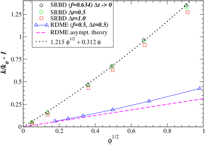
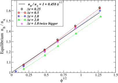
Figure 1: Conversion from microscopic to macroscopic reaction rates for (partially) diffusion-limited systems ($f=k_{0}/k_{S}\sim 1/2$) at finite packing densities $\phi$. Error bars are smaller or comparable to symbol size. (Left) Correction to the low-density rate $k_{0}$, given by (1) for SRBD and by (3) for RDME, for coagulation, $A+A\rightarrow A$ and $\emptyset\rightarrow A$. For SRBD, we use two different time step sizes (see legend) and extrapolate to the exact result without splitting errors. For the RDME an exact renormalization calculation gives the leading order non-analytic $\phi^{1/2}$ correction Coagulation_Renormalization_PRL ; Coagulation_Renormalization , which matches our numerical results for sufficiently small densities. For SRBD the result is well-fit by the empirical fit $k/k_{0}=1+1.215\phi^{1/2}+0.312\phi$ (dotted black line). (Right) Deviation $k/k_{0}=n_{B}/n_{A}$ from the low-density rate $k_{0}$ given by (1) for SRBD for annihilation, $A+B\rightarrow B$ and $\emptyset\rightarrow A$, for several time step sizes (see legend). For $\Delta t=1$ we show results obtained using a system that is twice larger (i.e., eight times the number of particles) and see no measurable finite-size effects. There is no theory for finite densities but the result is consistent with the empirical fit $k/k_{0}\approx 1+0.458\phi^{1/2}$.

For annihilation we consider a system with two species and the reactions $A+B\rightarrow B$ (i.e., conserved number of $B$ molecules) and $\emptyset\underset{k_{i}}{\rightarrow}A$. We change the number density of B molecules $n_{B}$ and wait until a steady state is reached at a specific average density $n_{A}$ of $A$ molecules. In this case we define a packing density as $\phi=\left(n_{A}+n_{B}\right)\cdot\left(4\pi R_{AB}^{3}/3\right)$. We set $R_{AB}=1$ and $\lambda=0.2387$ (giving $k_{\text{mix}}=1$), and $D_{A}=D_{B}=0.03255$, giving $r\approx 3.67$ and therefore $f=k_{0}/k_{S}^{\text{SRBD}}=0.5$. We set the rate of (random) insertion $k_{i}$ of $A$’s into the system to $k_{i}=k_{0}n_{B}^{2}$, so that if $k=k_{0}$ it would be that $n_{A}=n_{B}$ at equilibrium. Therefore, $kn_{A}n_{B}=k_{0}n_{B}^{2}$, giving $k/k_{0}=n_{B}/n_{A}$. In the right panel of Fig. 1 we compute the deviation of the measured reaction rate from the low-density prediction (1) via the ratio $n_{B}/n_{A}$ at several packing densities and for several values of the time step size. Again the results are consistent with a splitting error of order $O\left(\Delta t^{2}\right)$ (not shown), and for sufficiently small $\Delta t$ and $\phi\rightarrow 0$ the results are in perfect agreement with the theory (1). For finite densities, there is no known theory but we expect that for fixed composition (4) will hold with a different coefficient $\gamma$; indeed, the results appear to be consistent with a non-analytic $\phi^{1/2}$ dependence for small $\phi$.

III.2 Optimal Cell Size

We recall that, as far as accuracy is concerned, the choice of the grid cell size $h$ in SRBD is arbitrary beyond requiring $h\geq R_{\max}$. However, the choice of $h$ is crucial to the efficiency of the algorithm. We expect that there will be an optimal choice $h_{\text{opt}}$ that balances the increased costs of maintaining and building the grid data structures versus the benefits of reducing the number of particle pairs that need to be checked for overlap. If $h_{\text{opt}}<R_{\max}$ then we must set $h=R_{\max}$ in order to ensure correctness of the algorithm.

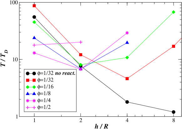
Figure 2: Ratio of SRBD computational time $T$ needed to simulate a reaction-diffusion process and the computational time $T_{D}$ needed to simulate diffusion-only process, as a function of cell size relative to reactive radius, for annihilation $A+B\rightarrow B$ and $\emptyset\rightarrow A$. We use the same parameters as used to produce Fig. 1, and set $\Delta t=1$, and employ system sizes ranging from 15.5 to 62 thousand particles. For low densities, an optimal cell size is observed ranging from $h=4R$ to $h=2R$. For densities $\phi\geq 1/2$, the minimum cost occurs for $h=R$ and the optimal grid size is the smallest possible one. For comparison, we include for $\phi=1/32$ results for the case when the reaction rates are set to zero so that they are still scheduled but never actually happen.

In Fig. 2 we show some empirical results on the cost of the SRBD algorithm as a function of the grid spacing. As a comparison, we use the computational time $T_{D}$ needed to diffuse the particles only, without processing any reactions. When we set the reaction rates to zero so that no reactions actually happen, managing the LLCs and event queue used to process reactions in SRBD (even though empty), increases the cost and it is optimal to set $h=L$, where $L$ is the system size. However, when reactions do happen, we see that the computational time is very sensitive to the choice of grid size $h$ and there is an optimal value $h_{\text{opt}}$ that minimizes the cost. As expected, for dilute systems it is best to set the cell size to be larger than the reactive radius, $h_{\text{opt}}>R_{\max}$, so that the cost is dominated by diffusion as particles try to find reactive partners, rather than being dominated by managing the grid-based data structures used in the SRBD algorithm. For larger densities however, the optimal choice is to make the cells as small as possible, $h_{\text{opt}}=R_{\max}$. The exact optimal value of $h$ will depend not only on details of the computational implementation and system size, but also on the reaction rates and densities in a nontrivial way, and we recommend that empirical testing is the best way to choose the optimal cell size in practice.

III.3 Long-time tails for reversible association $A+B\leftrightarrow C$

In this section we continue investigating diffusion-limited reactions at thermodynamic equilibrium in two dimensions. We focus here on the reversible association reaction $A+B\underset{k}{\rightarrow}C$ and $C\underset{\tilde{k}}{\rightarrow}A+B$, where the ratio of the forward and backward rate is chosen to give an equilibrium steady state with average number densities $\left\langle n_{A}\right\rangle=\left\langle n_{B}\right\rangle=\left\langle n_{C}\right\rangle=n$. In fact, SRBD reaches not just a steady state but a time-reversible state of true thermodynamic equilibrium. Recall that the microscopic association and dissociation mechanisms chosen in our Doi model formulation (see Section II.1.1) ensure detailed balance with respect to a uniformly mixed equilibrium distribution. This means that the steady state is a thermodynamic equilibrium state in which the $A$, $B$ and $C$ molecules are uniformly mixed in the domain and uncorrelated with one another. This implies that the forward reaction rate for the association is $k=\pi R_{AB}^{2}\lambda$ as if the system were reaction-limited and thus locally well-mixed. This holds independently of the value of $\lambda$, i.e., independently of whether the reaction is actually diffusion-limited or reaction-limited.

However, the unusual macroscopic behavior of the system for diffusion-limited parameters becomes evident if one considers not the static or instantaneous rate, but rather, the dynamics of the fluctuations around the equilibrium values. In particular, it has been known for some time that the microscopic reaction mechanism affects the autocorrelation function (ACF) of the fluctuations in the number density,

$$\text{ACF}(t)=\left\langle\left(n_{C}(\tau+t)-n\right)\left(n_{C}(\tau)-n\right)\right\rangle,$$

where $n_{C}(t)=N_{C}(t)/V$ is the instantaneous number density averaged over the spatial extent of the domain. If the system were reaction-limited and the usual law of mass action kinetics applied, the ACF would show exponential decay, $\text{ACF}\left(t\right)\sim\exp\left(-3knt\right)$. However, when the reaction is diffusion-limited, one observes a long-time power-law tail in the ACF LongTimeTails_ABC ; AsymptoticPowerLaw_ABC ,

$$\text{ACF}\left(t\right)\approx\frac{5}{216n\pi Dt}\,\text{ACF}\left(0\right),$$ (5)

where for simplicity we have assumed equal diffusion coefficient for all species, $D_{A/B/C}=D$. The fundamental physics behind this long-time tail is the fact that the reaction locally conserves $\tilde{n}=n_{A}+n_{B}+2n_{C}$, which can only relax by slow diffusion. It is important to note that the asymptotic behavior (5) is independent of the reaction rate, i.e., independent of $\lambda$. Therefore, the ACF switches at some characteristic time $\tau$ from exponential behavior $\text{ACF}\left(t\ll\tau\right)\sim\exp\left(-3knt\right)$ with decay rate independent of $\lambda$, to an inverse time decay (5) with coefficient independent of $\lambda$ at long times. The value of $\lambda$ determines the value of $\tau$. For slow reactions, i.e., the reaction-limited case, exponential decay dominates over most of the decay. For fast reactions, i.e., the diffusion-limited case, the exponential decay lasts for only a very short amount of time, and the majority of the decay of the ACF is much slower than exponential.

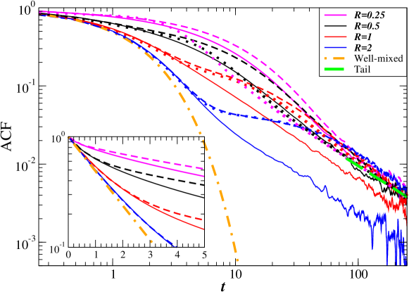
Figure 3: Autocorrelation function of the total number of $C$ molecules in a two-dimensional system undergoing the reversible association $A+B\leftrightarrow C$. Solid lines show results for SRBD with different values for the reactive radius $R$ (see legend), and dashed lines of the same color are for RDME with reactive grid spacing $h=2R$. The dotted lines are theoretical predictions for RDME based on fluctuating hydrodynamics LongTimeTails_ABC . The thick dashed dotted orange line shows the exponential decay predicted for a perfectly mixed system, and the thick dashed green line shows the theoretical tail (5). The inset focuses on early times and uses a linear scaling of the $x$ axis in order to emphasize the exponential decay observed in reaction-limited systems. Note that the long-time tail has non-negligible statistical noise compared to the signal when the ACF drops below $10^{-2}$.

In Fig. 3 we show the ACF for SRBD (solid lines) for several values of the reactive radius $R=R_{AB}=2R_{A}=2R_{B}$, for $n=0.23873$ particles per unit (two-dimensional) area, $D=0.032549$, $k=1$, $\tilde{k}=n$, for a square domain of length $L=64$ and time step size $\Delta t=0.25$. For each $R$, we show in the same color for comparison RDME (dashed lines) with a grid spacing $h=2R=4R_{A/B}$, which was determined empirically to lead to an excellent matching between SRBD and RDME at short to intermediate times. The inset in the figure focuses on short times and shows that $\text{ACF}\left(t\rightarrow 0^{+}\right)$ decays exponentially as predicted for a well-mixed (reaction-limited) system (orange dashed-dotted line). This is because SRBD reaches a steady state of thermodynamic equilibrium consistent with an ideal solution (gas) of $A$, $B$ and $C$ molecules. We have confirmed (not shown) that the two-particle (second order) correlation functions of our system are consistent with an ideal gas mixture to within statistical uncertainty.

For later times however, all of the ACFs shown in Fig. 3 show a much slower $t^{-1}$ decay than predicted for a well-mixed system. For RDME we see that the ACF has the same universal tail given by (5), shown as a thick dashed green line, independent of the value of the grid spacing $h$, as predicted by the theory. However, for SRBD, different values of the reactive distance $R$ lead to the same $t^{-1}$ decay at long times, but with a different coefficient. Empirically we find that fitting the SRBD tails with (5) gives an effective diffusion coefficient $D_{\text{eff}}=D+0.13knR^{2}.$ As already discussed in Section II.1.2, this enhancement of the effective diffusion coefficient by reactions comes because a sequence of association/dissociation reactions in SRBD leads to displacements of $A$ and $B$ molecules. Quite generally, we expect to see enhancement of the diffusion coefficients on the order of $\sim R^{2}/\tau$, where $\tau$ is a reactive time for the sequence $A+B\rightarrow C\rightarrow A+B$, but the exact dependence is difficult to compute analytically.

In LongTimeTails_ABC ; AsymptoticPowerLaw_ABC , Gopich et al. developed a perturbative (one-loop) renormalization theory for the tail of the ACF based on fluctuating hydrodynamics. In this theory, one assumes that the fluctuations are weak and solves the fluctuating hydrodynamics equations linearized around the equilibrium state, and then evaluates the nonlinear term due to the binary reactions to quadratic order in the fluctuations in order to estimate the leading-order corrections due to fluctuations. The theory is a continuum theory, but can be easily modified to account for the spatial discretization in RDME. Specifically, we have replaced the spectral (negative) Laplacian $q^{2}$ with the modified (negative) Laplacian $\sin^{2}\left(qh/2\right)/\left(h/2\right)^{2}$ in Eq. (3) in LongTimeTails_ABC , and replaced the integral over wavenumbers $\boldsymbol{q}$ in Eq. (11) in LongTimeTails_ABC with a sum over the discrete Fourier modes supported on the periodic RDME grid. The integral over time in Eq. (11) in LongTimeTails_ABC can be performed analytically, and the resulting sum over wavenumbers evaluated numerically. This gives a complete theory for $\text{ACF}(t)$, not just the tail computed explicitly in LongTimeTails_ABC . In Fig. 3 we show this theory with dotted lines for different values of the RDME grid spacing $h$. The improved theory is found to be in excellent agreement with the numerical data for $h=4$ (dark blue lines), with the agreement becoming progressively worse for smaller $h$, i.e., as the system becomes more and more diffusion-limited. By increasing the number density, i.e., the number of molecules per cell, we have confirmed that the mismatch with the theory for intermediate times for diffusion-limited reactions cannot be blamed on the fact that the fluctuations are not weak enough for the perturbation analysis to apply. Instead, it appears that the theory is missing some of the microscopic correlations that develop in diffusion-limited systems, revealing once again the difficulty of quantitative continuum modeling of such systems.

III.4 Pattern formation

In this section we study a two-dimensional reaction-limited system with three species $U$, $V$ and $W$, undergoing seven reactions according to the Baras-Pearson-Mansour (BPM) model Baras1990 ; Baras1996 ,

$$U+W \rightarrow V+W$$

$$V+V \leftrightarrows W$$

$$V \leftrightarrows 0$$

$$U \leftrightarrows 0.$$

The reaction rates are chosen to give a limit cycle for the reaction in the absence of diffusion, and the diffusion coefficient of the $U$ species is chosen to be very different, $D_{V}=D_{W}=D_{U}/10$, which leads to the formation of Turing-like spot patterns forming a hexagonal or a monoclinic structure (see Fig. 5 in FluctReactDiff ). A typical quasi steady-state pattern obtained for the parameters we use is illustrated in Fig. 4.

Figure 4: Typical Turing-like quasi-steady patterns for the BPM model at time $t=10^{4}$, illustrated here by color plots of the number densities for $U$ molecules. Left panel is for RDME, middle panel is for S-BD-RME, and right panel is for SRBD. The reactive distance is set to $R=h=0.125$, i.e., a $256^{2}$ grid, but the images were produced using a $64^{2}$ grid to compute local number densities, in order to reduce the fluctuations.

This system was studied using the RDME and fluctuating hydrodynamics by some of us in FluctReactDiff , and it was concluded that fluctuations accelerate the initial formation of a disordered spot pattern, and also accelerate the subsequent annealing of defects to form a lattice of spots. Here we repeat the same computations but using SRBD and S-BD-RME, in order to understand the importance of the microscopic model to the pattern formation. We have studied systems that are either initialized in a uniformly mixed state corresponding to a point on the limit cycle, which leads to initial oscillations of the average concentrations which get damped until a fixed Turing pattern is established, as well as systems initialized to be at the unstable fixed point of the limit cycle, so that fluctuations kick it onto the limit cycle via growing oscillations until eventually a fixed pattern forms. Here we focus on the setup studied in FluctReactDiff and initialize the system on the limit cycle; initially the particles of all three species are uniformly and randomly distributed throughout the domain.

We use the same reaction parameters as reported in Section VB in FluctReactDiff . Although the system is two-dimensional we think of it as a three-dimensional system with a small thickness $\Delta z=0.5$ in the third dimension , so that number densities are still expressed in units of particles per unit volume rather than per unit area. For simplicity, in SRBD we set $R_{U}=R_{V}=R_{W}=R/2$, where $R$ is the reactive distance. The chosen reaction rates and diffusion coefficients are such that the system is reaction-limited, so that we can easily obtain the effective macroscopic reaction rate for any binary reaction from the two-dimensional equivalent of (2) ,

$$k=s\left(\pi R^{2}\Delta z\right)\lambda.$$ (6)

This allows to obtain $\lambda$ for each reaction from the knowledge of the desired effective reaction rate $k$ for each of the three binary reactions in the BPM model. For S-BD-RME and RDME, we can simply use the desired effective rates $k$ as input microscopic rates, independent of the reactive cell size $h$. We vary $R$ and $h$ while keeping the overall system size fixed at $L_{x}=L_{y}=32$.

In SRBD we use the minimal possible grid spacing $h=R$ for sampling reactions, in order to maximize computational efficiency; in what follows we will use $h$ when comparing SRBD and RDME/S-BD-RME simulations but we remind the reader that $h$ has no physical meaning for SRBD. We change the grid size $N_{x}=N_{y}=L_{x}/h$ from $N_{x}=64$ to $N_{x}=512$; for the chosen rate parameters we would need grids larger than $1024\times 1024$ to enter the diffusion-limited regime. Our RDME computations are performed using the split scheme described in Appendix A of FluctReactDiff . The time step size $\Delta t$ for all methods is limited by the fast diffusion of $U$ molecules, and we set the diffusive Courant number to $D_{U}\Delta t/h^{2}\approx 0.3$. The total number of molecules (particles) in the system can be as large as $2.5\cdot 10^{6}\Delta z$, i.e., about a million particles for our setup. As a rough idea of the computational effort involved, we note that for $N_{x}=256$, the total running time up to physical time $T=10^{4}$ on a 3GHz Intel Xeon processor was 4.5h for RDME, 12h for S-BD-RME, and 19h for SRBD. For $N_{x}=512$, the running time was 54h for S-BD-RME and 48h for SRBD, which decreased to 43h when a $256^{2}$ grid was used to process the reactions in SRBD (see discussion in Section III.2).

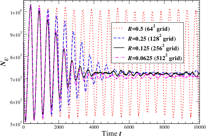
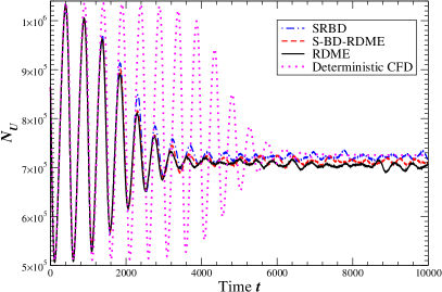
Figure 5: Total number $N_{U}\left(t\right)$ of $U$ molecules in a pattern-forming BPM reaction-diffusion model in two dimensions. Initially $N_{U}$ oscillates on the limit cycle of the reaction-only model, until a Turing-like spatial instability leads to the formation of a quasi-steady spot pattern. (Left) Results for SRBD for different values of the reactive distance $R$ (see legend). The computations used a grid (size shown in legend) of spacing $h=R$ for processing reactions. (Right) Comparison between SRBD with $R=0.125$ to S-BD-RME and RDME with reactive grid spacing $h=R=0.125$. The pattern formation is delayed for deterministic CFD FluctReactDiff on a grid of spacing $h=0.125$, initialized with a statistically indistinguishable initial condition.

In Fig. 5, we show the total number of $U$ molecules as a function of physical time. This number oscillates according to the limit cycle for a while, until a quasi-steady pattern is formed. The types of “steady” Turing-like patterns obtained using SRBD and S-BD-RME are visually indistinguishable from those obtained using RDME, as illustrated in Fig. 4. In the presence of fluctuations the final patterns are not strictly stationary and the Turing spots can diffuse, however, this happens on a slow time scale not studied here. Of main interest to us is the typical time it takes for the Turing pattern to emerge.

In the left panel of Fig. 5, we show results for SRBD for four different values of the particle diameter $R$. Somewhat unexpectedly, the results for S-BD-RME with grid spacing $h=R$ were found to be visually indistinguishable from those for SRBD with reactive radius $R$. For SRBD or S-BD-RME, we do not see a Turing pattern emerging even after $t=10^{5}$ when $R=0.5$. By contrast, a pattern is formed in less time even if the deterministic reaction-diffusion equations (corresponding to the limit $\Delta z\rightarrow\infty$) are solved using standard computational fluid dynamics (CFD) techniques FluctReactDiff starting from a random initial condition. A pattern does form for SRBD for $R=0.25$, and it forms faster yet for $R=0.125$, and no noticeable change happens when we reduce the reactive distance even further to $R=0.0625$. Somewhat surprisingly, the results for RDME were found to be rather independent of the grid size, as also observed in Fig. 7 in FluctReactDiff , and are statistically hard to distinguish from those obtained using SRBD or S-BD-RME for $R\leq 0.125$, as illustrated in the right panel of Fig. 5.

We can explain the difference between RDME and SRBD/S-BD-RME by the observation that diffusion is enhanced by reactions in methods in which diffusion takes place off lattice, as we discussed in Section II.1.2 and quantified in Section III.3. Indeed, the formation of the pattern can be suppressed also by enlarging the diffusion coefficients of the particles in RDME. Since the effective enlargement of the diffusion coefficients in SRBD/S-BD-RME is proportional to $R^{2}$, using smaller reactive radii makes the effect smaller.

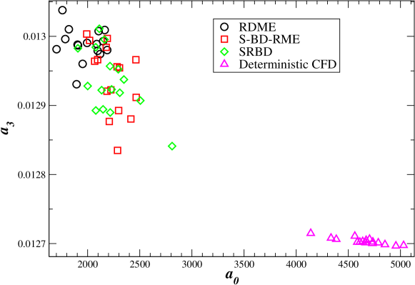
Figure 6: Scatter plot of the fitting coefficients $a_{0}$ and $a_{3}$ in the empirical fit (7) for the dynamics of pattern formation in the BPM model, for 16 statistically independent simulations using one of four different methods (see legend).

We can make the comparison between the different methods for $R=0.125$ more quantitative by fitting the total number of $U$ molecules as a function of time to the empirical fit (see Eq. (41) in FluctReactDiff )

$$N_{U}(t)=\left(1-\tanh\left((t-a_{0})/a_{2}\right)\right)\left(a_{1}\,\sin(a_{3}t+a_{4})+a_{5}\right)+a_{6},$$ (7)

and comparing the distribution of the fitting parameters for the different methods over a set of statistically-independent runs. This comparison is shown in Fig. 6. In this figure we show the values of the fitting parameters $a_{0}$, which represents the onset time for the pattern formation, and $a_{3}$, which represents the frequency of the oscillation, for 16 samples initialized using statistically independent random configurations and using different random number streams, for RDME, S-BD-RME, SRBD and deterministic CFD. Each of the methods forms a cluster in this plane, and it is clear that deterministic CFD is quite distinct in both the onset time and the frequency (note, however, that the range of the $y$ axis is rather small) from the methods that account for fluctuations. All methods that include fluctuations are relatively similar in this comparison, but the RDME cluster is seen to be somewhat separated from SRBD and S-BD-RME, which are themselves not distinguishable in this statistical test. We believe that the small difference between RDME and SRBD/S-BD-RME stems from the slightly enhanced diffusion in the Doi model compared to lattice-based models.

IV Conclusions and Future Directions

We described a novel method for simulating the Doi or volume reactivity model of reaction-diffusion systems. The SRBD algorithm is based on time splitting of diffusion and reaction, and uses an event-driven algorithm to schedule and process reactions during a time step without any approximations. This makes the method robust from the reaction-limited to the diffusion-limited case, and allows one to easily control the numerical error in SRBD by reducing the time step size. Unlike simpler algorithms for incorporating thermal fluctuations in reaction-diffusion models, such as the widely-used RDME, a grid is only used in SRBD to dramatically improve computational efficiency, without affecting physical observables. The SRBD method is therefore a true particle method that maintains Galilean invariance and isotropy, just like molecular dynamics.

Our studies of irreversible association in Section III.1 showed the complexity of the conversion from microscopic to effective macroscopic rates for diffusion-limited reactions. Such conversion is in fact not possible in two dimensions, and even in three dimensions the corrections to the effective rate depend non-analytically on the density Coagulation_Renormalization_PRL ; Coagulation_Renormalization . This brings into question the law of mass action kinetics for diffusion-limited systems, even at macroscopic length and time scales, casting doubts on any attempt to model such systems using local in space and time reaction-diffusion equations. Our studies of diffusion-limited reversible association in Section III.3 indicated that even though a simple law of mass action kinetics can model the instantaneous macroscopic reaction rate, long-lived temporal correlations of the fluctuations lead to effective memory in the dynamics RelaxationTime_ABC . Furthermore, we numerically demonstrated that by ensuring reversibility of the microscopic reaction rules we achieve a state of true thermodynamic equilibrium DiffusionLimited_NonDB .

For reaction-limited systems, diffusion is fast enough to mix the reactants at microscopic and mesoscopic scales, and the conversion from microscopic to macroscopic rates is much simpler. Indeed, in Section III.4 we found a good matching between the simpler and more efficient RDME model and SRBD/S-BD-RDME for sufficiently small reactive distances, for a system undergoing a pattern-forming Turing-like instability. Nevertheless, we found that when finite-range reactions are combined with off-lattice diffusion, reversible reactions increase the effective diffusion coefficient by an amount on the order of $R^{2}/\tau$, where $R$ is the typical reactive distance, and $\tau$ is the typical duration of a binding-unbinding sequence.

One can argue that the enhancement of the diffusion coefficients by reactions that we observed in the Doi model is unphysical, since one considers reaction and diffusion to be separate physical processes that cannot couple by the Curie principle. At the same time, for diffusion-limited systems reaction and diffusion are intimately coupled, and it is not in fact obvious that the traditional reaction-diffusion partial differential equation, in which reaction and diffusion are completely decoupled, is appropriate (even once rates are renormalized). Since diffusion affects macroscopic reaction rates, it is perhaps natural to expect that reactions should in turn affect diffusion on macroscopic scales.

The enhanced diffusion in the Doi model occurs because of the simplifications of actual reactive mechanisms. Notably, all molecules are considered to be point-like particles and only identified by a species label. When a forward reaction $A+B\rightarrow C$ takes place, all information about the original reactant particles is lost, and is subsequently stochastically re-created by the reverse reaction. This is equivalent to saying that once the $C\equiv AB$ complex forms, it rotates and rearranges internally on a much faster time scale than it diffuses, which is unphysical. In an actual reaction, however, the $A$ or $B$ will denote atomic units or molecular subunits that will retain their identity via the reaction, and a more physically-realistic model may treat the $C$ as a combination $A+B$ of units that are bonded by an elastic or rigid bond, thus retaining the rotational diffusion of the $C$ molecule (molecular complex), and the finite time scales of the internal dynamics of this complex. Developing more physically realistic microscopic models is well beyond the scope of the present work, but remains an important topic for future study. It should be noted that the key algorithmic ideas developed in this work can find use well beyond just the specific Doi model we employed in this work.

A key disadvantage of event-driven algorithms such as FPKMC and SRBD is the difficulty of parallelization of event loops without making uncontrolled approximations. The diffusion step in SRBD can be trivially parallelized since each particle diffuses independently of other particles. The parallelizaton of the reactive step, however, requires sophisticated “time-warp” technology only recently employed for kinetic Monte Carlo simulation Parallel_KMC_Bulatov . Future work should explore whether it is possible to parallelize SRBD using simpler techniques by using the fact that the time step size provides an upper bound on the maximum time to the next event.

In the SRBD model used in this work, we assumed that the particles are independent Brownian walkers. It is well-known that this model is not appropriate for particles diffusing in a liquid, because of the importance of long-ranged hydrodynamic correlations (often called hydrodynamic interactions) mediated by momentum transport in the solvent. The time splitting used in SRBD makes it very easy to use recently-developed linear-scaling Brownian Dynamics with Hydrodynamic Interactions (BD-HI) SpectralRPY to diffuse particles. This would enable studies of the importance of hydrodynamics to reaction-diffusion processes in crowded fluid environments such as the cell cytoplasm.

While the SRBD method is most powerful and efficient at higher densities, by changing the size of the grid used to accelerate the reaction handling one can also reasonably efficiently handle lower densities, as shown in Section III.2. Nevertheless, at very low densities the majority of the computing effort will be spent diffusing molecules, which will take a long time to find other molecules to react with. The problem of diffusing molecules rapidly over large distances without incurring any approximation errors is already elegantly solved by the FPKMC algorithm FPKMC_PRL ; FPKMC1 ; FPKMC2 . It is in fact possible to combine the FPKMC idea of propagating particles inside protective regions when they are far from other particles they could react with, with the SRBD handling for particles when they come close to each other. This can be accomplished relatively easily by adding to FPKMC a new kind of event, an SRBD time step, which is scheduled in regular intervals of $\Delta t$ to update those particles not protected by a domain by a time step of the SRBD algorithm. This kind of algorithm obviates the need for the complex handling of particle pairs in FPKMC while still retaining the key speedup of the FPKMC algorithm, and works naturally with the Doi reaction model even in regions of high densities. We leave such generalizations of the SRBD algorithm for future work.

Appendix

Appendix A Microscopic Reaction Rules

In this work, we adopt the following microscopic reaction rules based on classifying each reaction into one of several categories:

1. Death: $A\rightarrow\emptyset$. Every particle of species $A$ can disappear with rate $\lambda$ per unit time.

2. Birth: $\emptyset\rightarrow A$. With rate $\lambda$, a particle $A$ is created randomly and uniformly inside the domain. This reaction is the reverse of death.

3. Conversion: $A\rightarrow B$. Every particle of species $A$ has a rate $\lambda$ of changing species into $B$. This reaction is its own reverse (swapping the roles of $A$ and $B$).

4. Annihilation: $A+B\rightarrow\emptyset$ with rate $\lambda$ if within distance $R_{AB}$, where $B$ can be equal to $A$. Both particles disappear.

5. Production: $\emptyset\rightarrow A+B$. The particle of species $A$ is born randomly and uniformly in the domain (as for birth), and the particle of species $B$ is born with a random position uniformly distributed within a reactive sphere of radius $R_{AB}$ around the position of the particle of species $A$. This reaction is the reverse of annihilation.

6. Catalytic death: $A+B\rightarrow A$ with rate $\lambda$ if the $A$ and $B$ molecules are within distance $R_{AB}$. The particle of species $B$ disappears.

7. Catalytic birth: $A\rightarrow A+B$. Every particle of species $A$ has a rate $\lambda$ of splitting per unit time. A new particle of species $B$ is born with a random position uniformly distributed within a reactive sphere of radius $R_{AB}$ around the position of the particle of species $A$. This reaction is the reverse of catalytic death.

8. Binding: $A+B\rightarrow C$ with rate $\lambda$ if the $A$ and $B$ molecules are within distance $R_{AB}$, where we allow for $B$ to be equal to $A$, or for both $B$ and $C$ to be equal to $A$ (for example, as in coagulation $2A\rightarrow A_{2}$). One of the two reactants of species $A$ or $B$, chosen at random with probability $1/2$, changes species into $C$, and the other reactant particle disappears. Note that in specific applications it may be more appropriate to always convert the $A$ into $C$ instead of the random choice we implement here.

9. Unbinding: $A\rightarrow B+C$, where $B$ and/or $C$ can be equal to $A$. Every particle of species $A$ has a rate $\lambda$ of splitting per unit time. The particle of species $A$ becomes a product particle of species $B$ or $C$, chosen randomly with probability $1/2$ (see comment for binding about changes of this rule), and the second product particle is born randomly uniformly in a sphere centered at the $A$ with radius $R_{BC}$. This reaction is the reverse of coagulation.

10. Catalytic conversion: $A+B\rightarrow A+C$ with rate $\lambda$ if the $A$ and $B$ molecules are within distance $R_{AB}$, where $C$ can be equal to $A$. The particle of species $B$ changes species into $C$. This reaction is its own reverse.

11. Transformation: $A+B\rightarrow C+D$, with rate $\lambda$ if the $A$ and $B$ molecules are within distance $R_{AB}$. Here $B$ can be equal $A$, and $C$ and $D$ can both be equal to $A$ (i.e., the case of catalysis is excluded). One of the two reactant particles, chosen randomly with probability $1/2$, changes species into $C$, and the other reactant particle changes species into $D$. This reaction is its own reverse. Note that in specific applications it may be more appropriate to always convert the $A$ into $C$ and the $B$ into a $D$ instead of the random choice we implement here.

We note that we have combined here rules that could be simplified when some of the product/reactant species are identical for the sake of brevity. For example, one could give a more condensed reaction rule (and our code implements such condensed rules for efficiency) for reactions such as $A+A\leftrightarrow A$ or $A+A\leftrightarrow A+B$.

References

- (1) M. Dobrzynski, J.V. Rodriguez, J.A. Kaandorp, and J.G. Blom. Computational methods for diffusion-influenced biochemical reactions. Bioinformatics, 23(15):1969, 2007.
- (2) Anel Mahmutovic, David Fange, Otto G Berg, and Johan Elf. Lost in presumption: stochastic reactions in spatial models. Nature methods, 9(12):1163–1166, December 2012.
- (3) K. Kang and S. Redner. Scaling approach for the kinetics of recombination processes. Phys. Rev. Lett., 52:955–958, 1984.
- (4) Anton A. Winkler and Erwin Frey. Long-range and many-body effects in coagulation processes. Phys. Rev. E, 87:022136, Feb 2013.
- (5) Irina V Gopich, Alexander A Ovchinnikov, and Attila Szabo. Long-time tails in the kinetics of reversible bimolecular reactions. Phys. Rev. Lett., 86(5):922, 2001.
- (6) Irina V Gopich and Attila Szabo. Asymptotic relaxation of reversible bimolecular chemical reactions. Chemical physics, 284(1):91–102, 2002.
- (7) A Lemarchand and B Nowakowski. Do the internal fluctuations blur or enhance axial segmentation? EPL (Europhysics Letters), 94(4):48004, 2011.
- (8) P Dziekan, L Signon, B Nowakowski, and A Lemarchand. Reaction-diffusion approach to prevertebrae formation: Effect of a local source of morphogen. The Journal of chemical physics, 139(11):114107, 2013.
- (9) Yang Cao and Radek Erban. Stochastic turing patterns: analysis of compartment-based approaches. Bulletin of mathematical biology, 76(12):3051–3069, 2014.
- (10) Fu Zheng-Ping, Xu Xin-Hang, Wang Hong-Li, and Ouyang Qi. Stochastic simulation of turing patterns. Chinese Physics Letters, 25(4):1220, 2008.
- (11) Piotr Dziekan, J. S. Hansen, and Bogdan Nowakowski. Nanoscale turing structures. The Journal of Chemical Physics, 141(12):–, 2014.
- (12) Doriano Brogioli. Marginally stable chemical systems as precursors of life. Phys. Rev. Lett., 105:058102, 2010.
- (13) Doriano Brogioli. Marginal stability in chemical systems and its relevance in the origin of life. Phys. Rev. E, 84:031931, 2011.
- (14) Doriano Brogioli. Violation of the mass-action law in dilute chemical systems. The Journal of Chemical Physics, 139(18):184102, 2013.
- (15) Radek Erban, Jonathan Chapman, and Philip Maini. A practical guide to stochastic simulations of reaction-diffusion processes. arXiv preprint arXiv:0704.1908, 2007.
- (16) M. Malek-Mansour and G. Nicolis. A master equation description of local fluctuations. Journal of Statistical Physics, 13(3):197–217, 1975.
- (17) J. Keizer. Statistical thermodynamics of nonequilibrium processes. Springer, 1987.
- (18) C. W. Gardiner. Handbook of stochastic methods: for physics, chemistry & the natural sciences, volume Vol. 13 of Series in synergetics. Springer, third edition, 2003.
- (19) N. G. van Kampen. Stochastic Processes in Physics and Chemistry. Elsevier, third edition, 2007.
- (20) Daniel T. Gillespie. Stochastic simulation of chemical kinetics. Annual Review of Physical Chemistry, 58(1):35–55, 2007.
- (21) Johan Hattne, David Fange, and Johan Elf. Stochastic reaction-diffusion simulation with mesord. Bioinformatics, 21(12):2923–2924, 2005.
- (22) S. Lampoudi, D.T. Gillespie, and L.R. Petzold. The multinomial simulation algorithm for discrete stochastic simulation of reaction-diffusion systems. J. Chem. Phys., 130:094104, 2009.
- (23) Ariel Balter and Alexandre M Tartakovsky. Multinomial diffusion equation. Physical Review E, 83(6):061143, 2011.
- (24) C. Kim, A. J. Nonaka, A. L. Garcia, J. B. Bell, and A. Donev. Stochastic simulation of reaction-diffusion systems: A fluctuating-hydrodynamics approach. J. Chem. Phys., 146(12), 2017. Software available at https://github.com/BoxLib-Codes/FHD_ReactDiff.
- (25) David Fange, Otto G Berg, Paul Sjöberg, and Johan Elf. Stochastic reaction-diffusion kinetics in the microscopic limit. Proceedings of the National Academy of Sciences, 107(46):19820–19825, 2010.
- (26) Stefan Hellander, Andreas Hellander, and Linda Petzold. Reaction rates for mesoscopic reaction-diffusion kinetics. Phys. Rev. E, 91:023312, 2015.
- (27) Samuel A. Isaacson. A convergent reaction-diffusion master equation. The Journal of Chemical Physics, 139(5):–, 2013.
- (28) Masao Doi. Stochastic theory of diffusion-controlled reaction. Journal of Physics A: Mathematical and General, 9(9):1479, 1976.
- (29) Radek Erban and S Jonathan Chapman. Stochastic modelling of reaction–diffusion processes: algorithms for bimolecular reactions. Physical biology, 6(4):046001, 2009.
- (30) Anton A. Winkler and Erwin Frey. Validity of the law of mass action in three-dimensional coagulation processes. Phys. Rev. Lett., 108:108301, 2012.
- (31) Uwe C Täuber, Martin Howard, and Benjamin P Vollmayr-Lee. Applications of field-theoretic renormalization group methods to reaction–diffusion problems. Journal of Physics A: Mathematical and General, 38(17):R79, 2005.
- (32) Frank C Collins and George E Kimball. Diffusion-controlled reaction rates. Journal of colloid science, 4(4):425–437, 1949.
- (33) Noam Agmon. Diffusion with back reaction. The Journal of Chemical Physics, 81(6):2811–2817, 1984.
- (34) Hyojoon Kim and Kook Joe Shin. Exact solution of the reversible diffusion-influenced reaction for an isolated pair in three dimensions. Physical review letters, 82(7):1578, 1999.
- (35) Mauricio J del Razo and Hong Qian. A discrete stochastic formulation for reversible bimolecular reactions via diffusion encounter. Communications in Mathematical Sciences, 14(6):1741–1772, 2016.
- (36) Thorsten Prüstel and Martin Meier-Schellersheim. Exact green’s function of the reversible diffusion-influenced reaction for an isolated pair in two dimensions. The Journal of chemical physics, 137(5):054104, 2012.
- (37) T. Oppelstrup, V. V. Bulatov, G. H. Gilmer, M. H. Kalos, and B. Sadigh. First-Passage Monte Carlo Algorithm: Diffusion without All the Hops. Phys. Rev. Lett., 97(23):230602, 2006.
- (38) T. Oppelstrup, V. V. Bulatov, A. Donev, M. H. Kalos, G. H. Gilmer, and B. Sadigh. First-Passage Kinetic Monte Carlo Method. Phys. Rev. E, 80(6):066701, 2009.
- (39) A. Donev, V. V. Bulatov, T. Oppelstrup, G. H. Gilmer, B. Sadigh, and M. H. Kalos. A First-Passage Kinetic Monte Carlo Algorithm for Complex Diffusion-Reaction Systems. J. Comp. Phys., 229(9):3214–3236, 2010.
- (40) Ava J Mauro, Jon Karl Sigurdsson, Justin Shrake, Paul J Atzberger, and Samuel A Isaacson. A first-passage kinetic monte carlo method for reaction–drift–diffusion processes. J. Comp. Phys., 259:536–567, 2014.
- (41) Andri Bezzola, Benjamin B Bales, Richard C Alkire, and Linda R Petzold. An exact and efficient first passage time algorithm for reaction–diffusion processes on a 2d-lattice. J. Comp. Phys., 256:183–197, 2014.
- (42) Jeroen S. van Zon and Pieter Rein ten Wolde. Simulating biochemical networks at the particle level and in time and space: Green’s function reaction dynamics. Phys. Rev. Lett., 94:128103, 2005.
- (43) J. S. van Zon and P. R. ten Wolde. Green’s-function reaction dynamics: A particle-based approach for simulating biochemical networks in time and space. J. Chem. Phys., 123(23):234910, 2005.
- (44) M. H. Kalos, D. Levesque, and L. Verlet. Helium at zero temperature with hard-sphere and other forces. Phys. Rev. A, 9(5):2178–2195, 1974.
- (45) Steven S. Andrews, Nathan J. Addy, Roger Brent, and Adam P. Arkin. Detailed simulations of cell biology with smoldyn 2.1. PLoS Comput Biol, 6(3):e1000705, 03 2010.
- (46) David Fange, Anel Mahmutovic, and Johan Elf. Mesord 1.0: Stochastic reaction-diffusion simulations in the microscopic limit. Bioinformatics, 28(23):3155–3157, 2012.
- (47) Johann Biedermann, Alexander Ullrich, Johannes Schöneberg, and Frank Noé. Readdymm: Fast interacting particle reaction-diffusion simulations using graphical processing units. Biophysical journal, 108(3):457–461, 2015.
- (48) Martin Robinson, Mark Flegg, and Radek Erban. Adaptive two-regime method: application to front propagation. The Journal of chemical physics, 140(12):124109, 2014.
- (49) A. Donev, A. L. Garcia, and B. J. Alder. Stochastic Hard-Sphere Dynamics for Hydrodynamics of Non-Ideal Fluids. Phys. Rev. Lett, 101:075902, 2008.
- (50) A. Donev, A. L. Garcia, and B. J. Alder. A Thermodynamically-Consistent Non-Ideal Stochastic Hard-Sphere Fluid. J. of Statistical Mechanics: Theory and Experiment, 2009(11):P11008, 2009.
- (51) A. Donev, T. G. Fai, and E. Vanden-Eijnden. A reversible mesoscopic model of diffusion in liquids: from giant fluctuations to Fick’s law. Journal of Statistical Mechanics: Theory and Experiment, 2014(4):P04004, 2014.
- (52) TaiJung Choi, Mano Ram Maurya, Daniel M Tartakovsky, and Shankar Subramaniam. Stochastic operator-splitting method for reaction-diffusion systems. The Journal of chemical physics, 137(18):184102, 2012.
- (53) G. Gompper, T. Ihle, D. Kroll, and R. Winkler. Multi-Particle Collision Dynamics: A Particle-Based Mesoscale Simulation Approach to the Hydrodynamics of Complex Fluids. Advanced Computer Simulation Approaches for Soft Matter Sciences III, pages 1–87, 2009.
- (54) R Voituriez, M Moreau, and G Oshanin. Reversible diffusion-limited reactions:“chemical equilibrium” state and the law of mass action revisited. EPL (Europhysics Letters), 69(2):177, 2005.
- (55) Jana Lipková, Konstantinos C Zygalakis, S Jonathan Chapman, and Radek Erban. Analysis of brownian dynamics simulations of reversible bimolecular reactions. SIAM Journal on Applied Mathematics, 71(3):714–730, 2011.
- (56) A. Donev. Asynchronous event-driven particle algorithms. SIMULATION: Transactions of The Society for Modeling and Simulation International, 85(4):229–242, 2008.
- (57) M. P. Allen and D. J. Tildesley. Computer Simulations of Liquids. Oxford Science Publications, 1987.
- (58) Irina V. Gopich and Attila Szabo. Kinetics of reversible diffusion influenced reactions: The self-consistent relaxation time approximation. The Journal of Chemical Physics, 117(2):507–517, 2002.
- (59) D. Zhong, R. Dawkins, and D. ben Avraham. Large-scale simulations of diffusion-limited n-species annihilation. Phys. Rev. E, 67(4):040101, 2003.
- (60) F. Baras, J. E. Pearson, and M. Malek Mansour. Microscopic simulation of chemical oscillations in homogeneous systems. The Journal of Chemical Physics, 93(8):5747–5750, 1990.
- (61) F. Baras, M. Malek Mansour, and J. E. Pearson. Microscopic simulation of chemical bistability in homogeneous system s. The Journal of Chemical Physics, 105(18):8257–8261, 1996.
- (62) Tomas Oppelstrup, David R Jefferson, Vasily V Bulatov, and Luis A Zepeda-Ruiz. Spock: Exact parallel kinetic monte-carlo on 1.5 million tasks. In Proceedings of the 2016 annual ACM Conference on SIGSIM Principles of Advanced Discrete Simulation, pages 127–130. ACM, 2016.
- (63) A. M. Fiore, F. Balboa Usabiaga, A. Donev, and J. W. Swan. Rapid sampling of stochastic displacements in brownian dynamics simulations. J. Chem. Phys., 146(12):124116, 2017. Software available at https://github.com/stochasticHydroTools/PSE.
- (64) Koichi Takahashi, Sorin Tănase-Nicola, and Pieter Rein Ten Wolde. Spatio-temporal correlations can drastically change the response of a mapk pathway. Proceedings of the National Academy of Sciences, 107(6):2473–2478, 2010.