A New Proof for a Triple Product Formula for Plane Partitions

Abstract

Stanley generalized MacMahon’s classical theorem by proving a product formula for the norm-trace generating function for plane partition with unbounded parts. In his recent work on biothorgonal polynomials, Kamioka proved a finite analogue of Stanley’s formula for plane partitions with bounded parts (arXiv:1508.01674). In this paper, we use techniques from the enumeration of tilings to give a new proof for Kamioka’s formula.

Keywords: plane partitions, perfect matchings, lozenge tilings, dual graphs, graphical condensation.

1 Introduction

A partition $\lambda$ of $n$ to be non-increasing sequence of positive integers $(\lambda_{1},\lambda_{2},\dotsc,\lambda_{r})$ such that $\lambda_{1}+\lambda_{2}+\dotsc+\lambda_{r}=n$. Given a partition $\lambda=(\lambda_{1},\lambda_{2},\dotsc,\lambda_{r})$ of $n$, a plane partition of $n$ with the shape $\lambda=(\lambda_{1},\lambda_{2},\dotsc,\lambda_{r})$ is an array of non-negative integers of the form

$$\pi=\begin{tabular}[]{rccccccccc}$\pi_{1,1}$&$\pi_{1,2}$&$\pi_{1,3}$&$\dotsc$&$\dotsc$&$\dotsc$&$\pi_{1,\lambda_{1}}$\\ \vskip 3.0pt plus 1.0pt minus 1.0pt\vskip 3.0pt plus 1.0pt minus 1.0pt\cr$\pi_{2,1}$&$\pi_{2,2}$&$\pi_{2,3}$&$\dotsc$&$\dotsc$&$\pi_{2,\lambda_{2}}$&\\ \vskip 3.0pt plus 1.0pt minus 1.0pt\vskip 3.0pt plus 1.0pt minus 1.0pt\cr$\vdots$&$\vdots$&$\vdots$&$\vdots$&\reflectbox{$\ddots$\quad}&&\\ \vskip 3.0pt plus 1.0pt minus 1.0pt\vskip 3.0pt plus 1.0pt minus 1.0pt\cr$\pi_{r,1}$&$\pi_{r,2}$&$\pi_{r,3}$&$\dotsc$&$\pi_{r,\lambda_{r}}$&&\\ \vskip 3.0pt plus 1.0pt minus 1.0pt\vskip 3.0pt plus 1.0pt minus 1.0pt\cr\end{tabular},$$ (1.1)

where all rows and columns are weakly decreasing from left to right and from top to bottom, respectively. The norm (or the volume) $|\pi|$ of the plane partition $\pi$ is defined to be the sum of all entries in $\pi$. The entries in $\pi_{i,j}$ are called the parts of $\pi$.

Denote by $\mathcal{P}(r,c,n)$ the set of all plane partitions having at most $r$ rows, $c$ columns, and the maximal part $\pi_{1,1}$ at most $n$. MacMahon [10] showed that the norm generating function of plane partitions in $\mathcal{P}(r,c,n)$ is given by the following triple product

$$\sum_{\pi\in\mathcal{P}(r,c,n)}q^{|\pi|}=\prod_{i=1}^{r}\prod_{i=1}^{c}\prod_{i=1}^{n}\frac{1-q^{i+j+k-1}}{1-q^{i+j+k-2}}.$$ (1.2)

By letting $n\rightarrow\infty$, we obtain the norm generating function for the plane partitions with unbounded parts

$$\sum_{\pi\in\mathcal{P}(r,c)}q^{|\pi|}=\prod_{i=1}^{r}\prod_{i=1}^{c}\frac{1}{1-q^{i+j-1}},$$ (1.3)

where $\mathcal{P}(r,c)$ denotes the set of plane partitions with at most $r$ rows and $c$ columns.

Stanley [11] generalized (1.3) by introducing the trace of the plane partition $\pi$

$$\operatorname{tr}(\pi):=\sum_{i=1}\pi_{i,i}$$ (1.4)

and proving a closed form product formula for the norm-trace generating function

$$\sum_{\pi\in\mathcal{P}(r,c)}q^{|\pi|}a^{\operatorname{tr}(\pi)}=\prod_{i=1}^{r}\prod_{i=1}^{c}\frac{1}{1-aq^{i+j-1}}.$$ (1.5)

A Young diagram $[\lambda]$ of a partition $\lambda=(\lambda_{1},\lambda_{2},\dotsc,\lambda_{r})$ (or of shape $\lambda=(\lambda_{1},\lambda_{2},\dotsc,\lambda_{r})$) is a collection of unit squares $(i,j)$ on a square grid $\mathbb{Z}^{2}$, with $1\leqslant i\leqslant r$ and $1\leqslant j\leqslant\lambda_{i}$ (see Figure 1.1(a)). We usually write the entries of a plane partition in a Young diagram of the same shape (see Figure 1.1(b)).

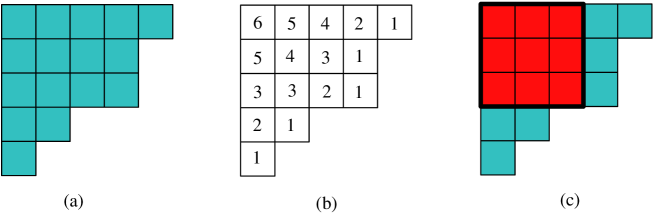
Figure 1.1: (a) Young diagram of shape (5,4,4,2,1). (b) A plane partition of the same shape. (c) Durfee square of a Young diagram.

The largest square $D=\{(i,j),1\leqslant i,j\leqslant r\}$ fitting in the Young diagram $[\lambda]$ is called the Durfee square of the Young diagram $[\lambda]$ (or of the partition $\lambda$) (see the square restricted by the bold contour in Figure 1.1(c))

For a plane partition $\pi$ of shape $\lambda$ and a number $1\leqslant k\leqslant\pi_{1,1}$, we define the $k$-truncation $\pi^{(k)}$ of $\pi$ to be the plane partition obtained from $\pi$ by removing all parts less than $k$ (see the plane partitions restricted in the contour in the left pictures in Figures 1.2(a)–(e)). We call the partition corresponding to the shape $\lambda$ of the plane partition $\pi^{(k)}$ the $k$-cross section of $\pi$, denoted by $\lambda^{(k)}(\pi)$ (see the right pictures in Figures 1.2(a)–(e) for $k=2,3,4,5,6$, respectively). It is obvious that $\pi^{(1)}=\pi$ and $\lambda^{(1)}(\pi)=\lambda$.

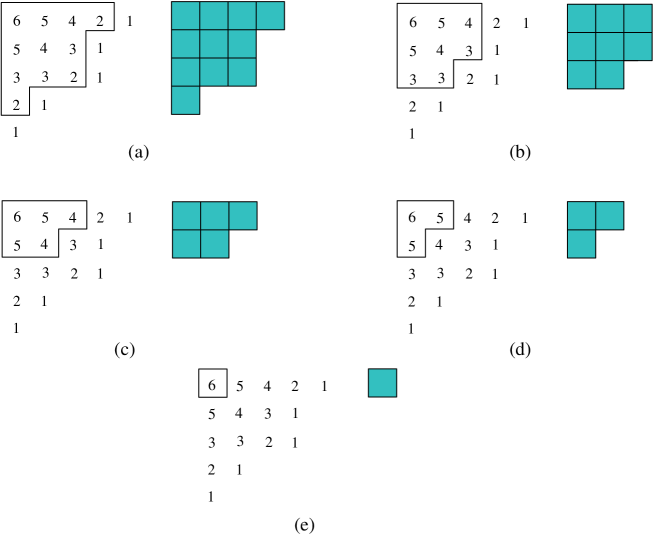
Figure 1.2: The $k$-truncations and the corresponding Young diagram of the $k$-cross sections of the plane partition in Figure 1.1, for (a) $k=2$, (b) $k=3$, (c) $k=4$, (d) $k=5$, and (e) $k=6$.

Recently, Kamioka [6] uses biorthogonal polynomials and lattice paths to prove a striking finite analogue of Stanley’s formula (1.5) for plane partitions in $\mathcal{P}(r,c,n)$.

Theorem 1.1.

Assume that $r,c,n$ are nonnegative integers. Then

$$\sum_{\pi}q^{|\pi|}a^{\operatorname{tr}(\pi)}\prod_{k=1}^{\pi_{1,1}}\frac{(q^{n-k+1};q)_{D_{k}(\pi)}}{(aq^{n-k+1};q)_{D_{k}(\pi)}}=\prod_{i=1}^{r}\prod_{j=1}^{c}\prod_{k=1}^{n}\frac{1-aq^{i+j+k-1}}{1-aq^{i+j+k-2}},$$ (1.6)

where

$$(x;q)_{N}=(1-x)(1-xq)\dots(1-xq^{N-1})$$

and where $D_{k}(\pi)$ is the size of the Durfee square of the $k$-truncation $\lambda^{(k)}(\pi)$ of $\pi$.

One readily sees that Kamioka’s formula also implies MacMahon’s classical formula (1.2) by specifying $a=1$.

The plane partitions in $\mathcal{P}(r,c,n)$ can be viewed as piles (or stacks) of unit cubes fitting in a $r\times c\times n$ box (see Figures 1.3(a)–(c)). The latter in turn are in bijection with the lozenge tilings of a semi-regular hexagon $H_{r,c,n}$ of sides $r,c,n,r,c,n$ (in cyclic order) on the triangular lattice (see Figures 1.3(c) and (d)). Here a lozenge is the union of any two unit equilateral triangles sharing an edge, and a lozenge tiling of a region is a covering of the region by lozenges so that there are no gaps and overlaps. In the view of this, MacMahon’s identity (1.2) and Kamioka’s identity (1.6) give triple product formulas for weighted sums of lozenge tilings of the semi-regular hexagon $H_{r,c,n}$. We refer the reader to [9] and [8] for more similar generalizations of the MacMahon formula (1.2).

The goal of this paper is using techniques in enumeration of tilings, in particular the graphical condensation introduced by Eric Kuo [7], to give a new proof for the triple-product formula (1.6).

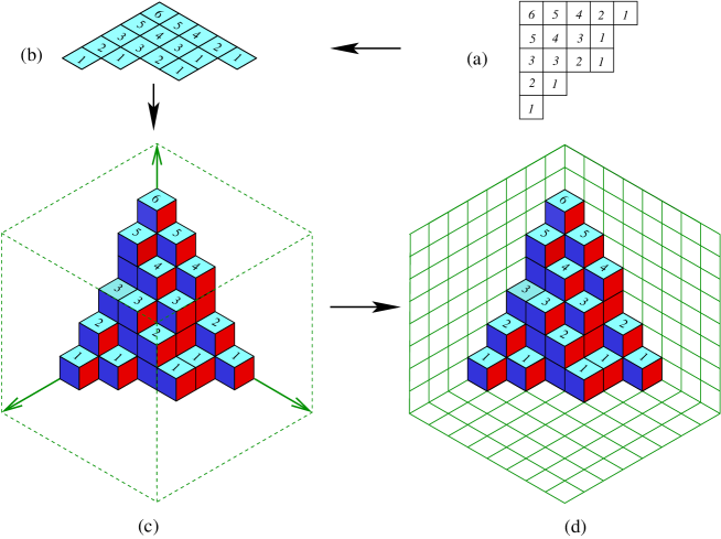
Figure 1.3: Bijection between plane partitions in $\mathcal{P}(8,8,8)$ and lozenge tilings of the hexagon $H_{8,8,8}$.

2 Preliminaries

Lozenges of a region can carry weights; and we define the weight of a lozenge tiling of the region to be the weight product of its lozenges. In the weighted case, we use the notation $\operatorname{M}(R)$ for the sum of weights of all lozenge tilings in $R$. We call $\operatorname{M}(R)$ a tiling generating function of $R$.

A forced lozenge of a region is the lozenge contained in any tiling of the region. Assume that one removes several forced lozenges $\ell_{1},\ell_{2},\dots,\ell_{k}$ from a region $R$ whose weights are $\operatorname{\textbf{wt}}(\ell_{1}),\operatorname{\textbf{wt}}(\ell_{2}),\dots,\operatorname{\textbf{wt}}(\ell_{k})$. We get a new region $R^{\prime}$ and obtain

$$\operatorname{M}(R)=\operatorname{M}(R^{\prime})\prod_{i=1}^{k}\operatorname{\textbf{wt}}(\ell_{i}).$$ (2.1)

A (perfect) matching of a graph $G$ is a collection of edges that cover each vertex exactly once. The dual graph $G$ of a region $R$ on the triangular lattice is the graph whose vertices are the unit triangles in $R$ and whose edges connect precisely two unit triangles sharing an edge. If lozenges in $R$ are weighted, we assign to each edge in the dual graph $G$ the same weight as that of its corresponding lozenge. Thus, one can identify the tilings of $R$ with the matchings of its dual graph $G$. In the view of this, we use the same notation $\operatorname{M}(G)$ for the sum of weights of all matchings in $G$, where the weight of a matchings is the weight product of its edges. We usually call $\operatorname{M}(G)$ a matching generating function of $G$.

In 2004, Eric Kuo [7] used a combinatorial interpretation of the well-known Dodgson condensation (or Desnanot-Jacobi identity, see e.g. [1]) to (re)prove the Aztec diamond theorem by Elkies, Kuperberg, Larsen and Propp [2, 3]. In particular, he proved the following condensation:

Theorem 2.1 (Theorem 5.1 in [7]).

Let $G=(V_{1},V_{2},E)$ be a (weighted) planar bipartite graph with $|V_{1}|=|V_{2}|$. Assume that $u,v,w,s$ are four vertices appearing in a cyclic order on a face of $G$. Assume in addition that $u,w\in V_{1}$ and $v,s\in V_{2}$. Then

$$\operatorname{M}(G)\operatorname{M}(G-\{u,v,w,s\})=\operatorname{M}(G-\{u,v\})\operatorname{M}(G-\{w,s\})+\operatorname{M}(G-\{u,s\})\operatorname{M}(G-\{v,w\}).$$ (2.2)

This theorem is the key of our proof in the next section.

3 New proof of Theorem 1.1

Lozenges have three orientations: left, right and horizontal as in Figure 3.1. We call the vertical line passing the north vertex of the semi-regular hexagon $H_{r,c,n}$ the axis of the hexagon (see the dotted line in Figure 3.5).

Figure 3.1: Three orientations of lozenges.

We first encode each plane partition $\pi$ in $\mathcal{P}(r,c,n)$ as a lozenge tiling of the semi-regular hexagon $H_{r,c,n}$ whose weight is $a^{\operatorname{tr}(\pi)}q^{|\pi|}$ as follows. View $\pi$ as a pile of $|\pi|$ unit cubes fitting in a $r\times c\times n$ box as in Figure 1.3. Here, each horizontal lozenge in the tiling corresponding to $\pi$ is pictured as the top of a column of unit cubes. We assign to each horizontal lozenge a weight $q^{h}$, where $h$ is the height of its corresponding column, except for the ones on the axis that are assigned a weight $(aq)^{h}$. All remaining lozenges are weighted by $1$. It is easy to see that the weight of the tiling is $a^{\operatorname{tr}(\pi)}q^{|\pi|}$. This weight assignment is called the natural $q$-weight assignment of the lozenge tiling.

For each horizontal lozenge $\ell$, we draw the vertical line passing the top and the bottom vertices of $\ell$. Assume that this vertical line passing $t$ other vertical lozenges above $\ell$ before meeting the northeast or northwest side of the hexagon. We say that $t$ is the depth of the horizontal lozenge $\ell$ (see Figure 3.2). It is easy to see that the depth $t$ of a horizontal lozenge on the $i$ lattice path and the height $h$ of the corresponding column of unit cubes are related by the following identity

$$t=n-h+(i-1).$$

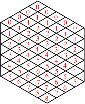
Figure 3.2: The depth of the lozenges in a hexagon.

One readily sees that the above weight assignment depends on the choice of the tilings. We would like to modify this weight assignment as follows.

First, we encode each tiling as a $r$-tuple of non intersecting lozenge paths connecting the northwest and southeast sides of the hexagon (see Figure 3.3; the lozenge paths consisting horizonal and right lozenges running along the dotted paths). Multiply the weight of horizontal lozenges on the $i$-th path (ordered from top to bottom) by $q^{-n-i+1}i$, the one intersect the vertical axis by $(aq)^{-n-i+1}$. Second, we multiply the weight of a horizontal lozenge on the $i$-th path that is passed through by the vertical axis by $\frac{(q^{n};q^{-1})_{n-t_{i}}}{(aq^{n};q^{-1})_{n-t_{i}}}$, where $t_{i}$ is the depth the lozenge. This way each horizontal lozenge is weighted by $q^{-t}$, and the one on the axis is weighted by $(aq)^{-t}\frac{(q^{n};q^{-1})_{n-t}}{(aq^{n};q^{-1})_{n-t}}$, where $t$ is the distance between the top of the horizontal lozenge and the southwest side of the hexagon. We denote by $\operatorname{\textbf{wt}}$ this new weight assignment; and this weight assignment does not depend on the choice of tiling.

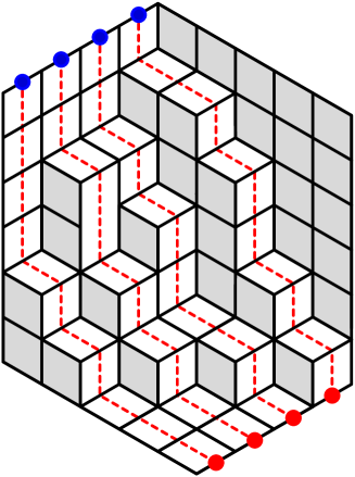
Figure 3.3: Encode each lozenge tiling of the hexagon $H_{3,5,6}$ as a $3$-tuples of distinct lozenge paths.

Lemma 3.1.

Let $\pi$ be any plane partition in $\mathcal{P}(r,c,n)$, and $T_{\pi}$ be the lozenge tiling of the hexagon $H_{r,c,n}$ corresponding to $\pi$. Then

$$A\operatorname{\textbf{wt}}(T_{\pi})=a^{-d(d+1)/2-(n+1)d}q^{-c(r(r+1)/2+(n-1)r)}q^{|\pi|}a^{tr(\pi)}w_{n}(\pi;a;q),$$ (3.1)

where $w_{n}(\pi,;a;q)=\prod_{k=1}^{\pi_{1,1}}\frac{(q^{n-k+1};q)_{D_{k}(\pi)}}{(aq^{n-k+1};q)_{D_{k}(\pi)}}$ as defined in Kamioka’s Theorem 1.1, $d=\min(r,c)$ is the number of horizontal lozenges on the vertical axis, and

$$A=\prod_{i=1}^{d}\frac{(aq^{n+i-1};q^{-1})_{i-1}}{(q^{n+i-1};q^{-1})_{i-1}}.$$

Proof.

We first assign the natural weight assignment on the lozenges of the tiling $T_{pi}$. The weight of the tiling $T_{\pi}$ is now $q^{|\pi|}a^{tr(\pi)}$. Next, we investigate how the weight of $T_{\pi}$ changes when we convert the natural weight of $T_{\pi}$ into the weight assignment $\operatorname{\textbf{wt}}$.

Consider the $r$-tuple of lozenge paths corresponding to the tiling $T_{\pi}$. Each lozenge path has exactly $c$ right lozenges, in which there is exactly one passed through by the vertical axis. Thus, the factor for the first step in the above weight modification is $a^{-d(d+1)/2-(n+1)d}q^{-c(r(r+1)/2+(n-1)r)}$.

Let us consider the factor for the second step. We write each factor $\frac{(q^{n-k+1};q)_{D_{k}(\pi)}}{(aq^{n-k+1};q)_{D_{k}(\pi)}}$ in $w_{n}(\pi,;a;q)$ as

$$w_{n}(\pi,a,q) =\prod_{k=1}^{\pi_{1,1}}\frac{(q^{n-k+1};q)_{D_{k}(\pi)}}{(aq^{n-k+1};q)_{D_{k}(\pi)}}=\prod_{k=1}^{\pi_{1,1}}\prod_{i=1}^{D_{k}(\pi)}\frac{1-q^{n-k+i}}{1-aq^{n-k+i}}$$

$$=\prod_{i=1}^{d}\prod_{k=1}^{h_{i}}\frac{1-q^{n-k+i}}{1-aq^{n-k+i}}=\prod_{i=1}^{d}\frac{(q^{n+i-1};q^{-1})_{h_{i}}}{(aq^{n+i-1};q^{-1})_{h_{i}}},$$ (3.2)

where $h_{i}$ the height of the column corresponding to the $i$-th horizontal lozenge on the vertical axis (ordered from the top to the bottom).

There are exactly $d=\min(r,c)$ right lozenges on the axis . The $i$-th one ($i=1,2,\dotsc,d$) from the top has weight

$$\frac{(aq^{n};q^{-1})_{n-t_{i}}}{(aq^{n};q^{-1})_{n-t_{i}}}=\frac{(q^{n+i-1};q^{-1})_{h_{i}}}{(aq^{n+i-1};q^{-1})_{h_{i}}}\cdot\frac{(aq^{n+i-1};q^{-1})_{i-1}}{(q^{n+i-1};q^{-1})_{i-1}}.$$ (3.3)

This implies that product of all the $d$ horizontal lozenges along the vertical axis is exactly $w_{n}(\pi,a,q)\times A$, where $A=\prod_{i=1}^{d}\frac{(aq^{n+i-1};q^{-1})_{i-1}}{(q^{n+i-1};q^{-1})_{i-1}}$.

Combining the factors in the two steps, we get

$$wt(T_{\pi})=Aa^{-d(d+1)/2-(n+1)d}q^{-c(r(r+1)/2+(n-1)r)}q^{|\pi|}a^{tr(\pi)}w_{n}(\pi;a;q)$$

∎

By the above lemma, in order to prove Kamioka’s theorem, we need to show that the tiling generating function of the hexagon $H_{r,c,n}$ weighted by $\operatorname{\textbf{wt}}$ is given by

$$\operatorname{M}(H_{r,c,n})=a^{-d(d+1)/2-(n+1)d}q^{-c(r(r+1)/2+(n-1)r)}A\prod_{i=1}^{r}\prod_{j=1}^{c}\prod_{k=1}^{n}\frac{1-aq^{i+j+k-1}}{1-aq^{i+j+k-2}}.$$ (3.4)

We prove (3.4) by induction on $r+c+n$. The base cases are the situations when at least one of $r,c,n$ equals to $0$. When $c=0$ or $r=0$, then $d=0$. It implies that all terms in the right-hand side of (3.4) are 1, and it is easy to see that the left-hand side is also 1. When $n=0$, the hexagon $H_{r,c,0}$ has only one tiling consisting all horizontal lozenges. Then the right-hand side of (3.4) is simply the weight product of all the horizontal lozenges, which is

$$a^{-d(d+1)/2-(n-1)d}q^{-c(r(r+1)/2+(n-1)r)} \prod_{i=1}^{d}\frac{(aq^{n+i-1};q^{-1})_{i-1}}{(q^{n+i-1};q^{-1})_{i-1}}$$ (3.5)

$$=a^{-d(d+1)/2-(n+1)d}q^{-c(r(r+1)/2+(n-1)r)}A.$$ (3.6)

This verifies the formula (3.4) in this case.

For induction step, we assume that (3.4) holds for any hexagon $H(r,c,n)$ in which the $r$-, $c$- and $n$-parameters are positive and whose sum is strictly less than $r+c+n$.

We apply Kuo condensation Theorem 2.1 to the dual graph $G$ of the hexagon $H_{r,c,n}$ weighted by $\operatorname{\textbf{wt}}$ as in Figure 3.4; the black triangles indicate the unit triangles corresponding to the four vertices $u,v,w,s$. In particular, the $u$-triangle is the black one on the southwest corner of the hexagon, and the $v$-, $w$-, and $s$-triangles are the black ones appearing respectively when we go counter-clockwise from the $u$-triangle.

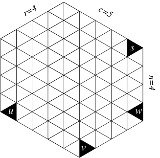
Figure 3.4: How we apply Kuo condensation.

Let us consider the region corresponding to the graph $G-\{u,v,w,s\}$. It has several forced lozenges. All of the forced lozenges have weight 1, except for $r-1$ horizontal ones long the southeast side of the hexagon, whose weights are $q^{-n},q^{-(n+1)},\dotsc,q^{-(n+r-2)}$ as they appear from right to left. Removing these forced lozenges, we get the hexagon $H_{r-1,c-1,n}$ weighted by $\operatorname{\textbf{wt}}$ (see Figure 3.5(b); the hexagon $H_{r-1,c-1,n}$ is indicated the the one with bold contour). Thus, we get

$$\operatorname{M}(G-\{u,v,w,s\})=q^{-(2n+r-2)(r-1)/2}\operatorname{M}(H_{r-1,c-1,n}).$$ (3.7)

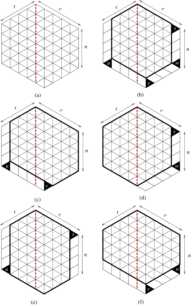
Figure 3.5: Obtaining the recurrence.

Similar, we remove the forced lozenges (which have all weight 1) in the region corresponding to $G-\{u,v\}$ and get a the hexagon $H_{r-1,c,n}$ weighted by $\operatorname{\textbf{wt}}$ (see Figure 3.5(c)).

$$\operatorname{M}(G-\{u,v\})=\operatorname{M}(H_{r-1,c,n}).$$ (3.8)

Next, if we remove forced lozenges with weight product $q^{-(2n+r-1)r}$ from the region corresponding to the graph $G-\{w,s\}$, we get the hexagon $H_{r,c-1,n}$ weighted by $\operatorname{\textbf{wt}}$ (see Figure 3.5(d)).

$$\operatorname{M}(G-\{w,s\})=q^{-(2n+r-1)r}\operatorname{M}(H_{r,c-1,n}).$$ (3.9)

The removal of forced lozenges (with weight 1) in the region corresponding to $G-\{u,s\}$ gives us the hexagon $H_{r-1,c-1,n+1}$ (illustrated in Figure 3.5(e)). Next, we divide the weight of each horizontal lozenges along the vertical axis by $\frac{(1-aq^{n+1})}{(1-q^{n+1})}$ to get the weight assignment $\operatorname{\textbf{wt}}$. Since each lozenge tiling of $H_{r-1,c-1,n+1}$ has exactly $d-1$ horizontal lozenges along the vertical axis, this changes the weight of each tiling of by a factor $\frac{(1-aq^{n+1})^{d-1}}{(1-q^{n+1})^{d-1}}$. Then we gat

$$\operatorname{M}(G-\{u,s\})=\frac{(1-aq^{n+1})^{d-1}}{(1-q^{n+1})^{d-1}}\operatorname{M}(H_{r-1,c-1,n+1}).$$ (3.10)

Finally, we get a weighted hexagon $H_{r,c,n-1}$ from the removal of forced lozenges from the region corresponding to $G-\{v,w\}$ (shown in Figure 3.5(f)). The weight product of the forced lozenges is $q^{-(2n+r-2)(r-1)/2}$. Next, we divide the weight of each horizontal lozenge on the vertical axis by $\frac{(1-q^{n})}{(1-aq^{n})}$ and get back the weight assignment $\operatorname{\textbf{wt}}$. Thus, we obtain

$$\operatorname{M}(G-\{v,w\})=q^{-(2n+r-2)(r-1)/2}\frac{(1-q^{n})^{d}}{(1-aq^{n})^{d}}\operatorname{M}(H_{r,c,n-1}).$$ (3.11)

Substituting the equations (3.7)–(3.11) into the equation (2.2) of Kuo’s Theorem 2.1, we have a recurrence on the tiling generating functions of the hexagons:

$$\operatorname{M}(H_{r,c,n})\operatorname{M}(H_{r-1,c-1,n})= q^{-n-r+1}\operatorname{M}(H_{r-1,c,n})\operatorname{M}(H_{r,c-1,n})$$

$$+\frac{(1-aq^{n+1})^{d-1}}{(1-q^{n+1})^{d-1}}\frac{(1-q^{n})^{d}}{(1-aq^{n})^{d}}\operatorname{M}(H_{r-1,c-1,n+1})\operatorname{M}(H_{r,c,n-1}).$$ (3.12)

Our final work is verifying that the expression on the right-hand side of (3.4) satisfies the same recurrence (3). Let $\phi(r,c,n)$ denote this expression, then we need to show that

$$\phi(r,c,n)\phi(r-1,c-1,n)= q^{-n-r+1}\phi(r-1,c,n)\phi(r,c-1,n)$$

$$+\frac{(1-aq^{n+1})^{d-1}}{(1-q^{n+1})^{d-1}}\frac{(1-q^{n})^{d}}{(1-aq^{n})^{d}}\phi(r-1,c-1,n+1)\phi(r,c,n-1)$$ (3.13)

or

$$q^{-n-r+1}\frac{\phi(r-1,c,n)}{\phi(r,c,n)} \frac{\phi(r,c-1,n)}{\phi(r-1,c-1,n)}$$

$$+\frac{(1-aq^{n+1})^{d-1}}{(1-q^{n+1})^{d-1}}\frac{(1-q^{n})^{d}}{(1-aq^{n})^{d}}\frac{\phi(r,c,n-1)}{\phi(r,c,n)}\frac{\phi(r-1,c-1,n+1)}{\phi(r-1,c-1,n)}=1.$$ (3.14)

We first simplify the fraction $\frac{\phi(r-1,c,n)}{\phi(r,c,n)}$ in the first term on the left-hand side of (3) as

$$\frac{\phi(r-1,c,n)}{\phi(r,c,n)} =\frac{q^{-c(r(r-1)/2+(n-1)(r-1))}}{q^{-c(r(r+1)/2+(n-1)r)}}\prod_{j=1}^{c}\prod_{k=1}^{n}\frac{1-aq^{r+j+k-2}}{1-aq^{r+j+k-1}}$$

$$=q^{c(n+r-1)}\prod_{j=1}^{c}\prod_{k=1}^{n}\frac{1-aq^{r+j+k-2}}{1-aq^{r+j+k-1}}.$$ (3.15)

Working similarly on the faction $\frac{\phi(r,c-1,n)}{\phi(r-1,c-1,n)}$ of the first term and multiplying the two fraction up, we obtain

$$\frac{\phi(r-1,c,n)}{\phi(r,c,n)}\frac{\phi(r,c-1,n)}{\phi(r-1,c-1,n)} =q^{n+r-1}\prod_{k=1}^{n}\frac{1-aq^{r+c+k-2}}{1-aq^{r+c+k-1}}$$

$$=q^{n+r-1}\frac{1-aq^{r+c-1}}{1-aq^{r+c+n-1}}.$$ (3.16)

We now simplify the fraction $\frac{\phi(r,c,n-1)}{\phi(r,c,n)}$ in the second term on the left-hand side of (3) as

$$\frac{\phi(r,c,n-1)}{\phi(r,c,n)} =a^{d}q^{cr}\prod_{i=1}^{d}\frac{1-aq^{n}}{1-aq^{n+i-1}}\frac{1-q^{n+i-1}}{1-q^{n}}$$

$$\times\prod_{i=1}^{r}\prod_{j=1}^{c}\frac{1-aq^{i+j+n-2}}{1-aq^{i+j+n-1}}.$$ (3.17)

Working similarly on the faction $\frac{\phi(r-1,c-1,n+1)}{\phi(r-1,c-1,n)}$ of the second term and multiplying these two fraction up, we get

$$\frac{\phi(r,c,n-1)}{\phi(r,c,n)}\frac{\phi(r-1,c-1,n+1)}{\phi(r-1,c-1,n)} =aq^{r+c-1}\frac{(1-aq^{n})^{d-1}}{(1-q^{n})^{d-1}}\frac{(1-q^{n+1})^{d-1}}{(1-aq^{n+1})^{d-1}}$$

$$\times\prod_{i=1}^{r}\prod_{j=1}^{c}\frac{1-aq^{i+j+n-2}}{1-aq^{i+j+n-1}}\prod_{i=1}^{r-1}\prod_{j=1}^{c-1}\frac{1-aq^{i+j+n}}{1-aq^{i+j+n-1}}$$

$$=aq^{r+c-1}\frac{(1-aq^{n})^{d-1}}{(1-q^{n})^{d-1}}\frac{(1-q^{n+1})^{d-1}}{(1-aq^{n+1})^{d-1}}\frac{(1-aq^{n})}{(1-aq^{r+c+n-1})}.$$ (3.18)

By (3) and (3), we now have

$$q^{-n-r+1}\frac{\phi(r-1,c,n)}{\phi(r,c,n)} \frac{\phi(r,c-1,n)}{\phi(r-1,c-1,n)}$$

$$+\frac{(1-aq^{n+1})^{d-1}}{(1-q^{n+1})^{d-1}}\frac{(1-q^{n})^{d}}{(1-aq^{n})^{d}}\frac{\phi(r,c,n-1)}{\phi(r,c,n)}\frac{\phi(r-1,c-1,n+1)}{\phi(r-1,c-1,n)}$$

$$=\frac{1-aq^{r+c-1}}{1-aq^{r+c+n-1}}+aq^{r+c-1}\frac{1-q^{n}}{1-aq^{r+c+n-1}}$$

$$=1.$$ (3.19)

This verifies (3) and finishes our proof.

4 Concluding Remarks

Gansner [4, 5] generalized Stanley’s trace formula by introducing the $\ell$-traces of the plane partition as $tr_{\ell}(\pi)=\sum_{i-j=\ell}\pi_{i,j}$. He showed that

$$\sum_{\pi\in\mathcal{P}(r,c)}\prod_{-r<\ell<c}=\prod_{i=0}^{r-1}\prod_{j=0}^{c-1}\left(1-\prod_{\ell=-i}^{j}q_{\ell}\right)^{-1}.$$ (4.1)

Kamioka also proved a finite analogue of Ganser’s formula (Theorem 17 in [6]). I believe that our method can be used to prove this theorem of Kamioka.

References

[1] C. L. Dodgson, Condensation of determinants, Proc. Roy. Soc. London
15 (1866), 150–155.
[2]
N. Elkies, G. Kuperberg, M. Larsen, and J. Propp,
Alternating-sign matrices and domino tilings (Part I), J. Algebraic Combin. 1 (1992), 111–132.
[3]
N. Elkies, G. Kuperberg, M. Larsen, and J. Propp,
Alternating-sign matrices and domino tilings (Part II), J. Algebraic Combin. 1 (1992), 219–234.
[4]
E. Gansner, The enumeration of plane partitions via the Burge correspondence, Illinois J. Math. 25 (1981), 533–554.
[5]
E. Gansner, The Hillman-Grassl correspondence and the enumeration of reverse plane partition, J. Comnbin. Theory Set. A 30 (1981), 71–89.
[6]
S. Kamioka, Plane partitions with bounded size of parts and biorthogonal polynomials (2015), Preprint arxiv:1508.01674. The preliminary version was published as “A triple product formula for plane partitions derived from biorthogonal polynomials”, DMTCS proc. BC, 2016, 671–682.
[7]
E. H. Kuo,
Applications of Graphical Condensation for Enumerating Matchings and Tilings,
Theor. Comput. Sci. 319 (2004),
29–57.
[8]
T. Lai,
A -enumeration of lozenge tilings of a hexagon with three dents, Adv. Applied Math 82 (2017), 23–57.
[9]
T. Lai,
A -enumeration of lozenge tilings of a hexagon with four adjacent triangles removed from the boundary, European J. Combin. 64 (2017), 66–87.
[10]
P. A. MacMahon,
Combinatory Analysis, Vol. 1 and 2,
Cambridge Univ. Press, 1916, reprinted by Chelsea, New York, 1960.
[11] R. Stanley, The conjugate trace and trace of a plane partition, J. Combin. Theory Ser. A 14 (1973), 53–65.