Goodness-of-fit tests for complete spatial randomness based on Minkowski functionals of binary images

Abstract

We propose a class of goodness-of-fit tests for complete spatial randomness (CSR). In contrast to standard tests, our procedure utilizes a transformation of the data to a binary image, which is then characterized by geometric functionals. Under a suitable limiting regime, we derive the asymptotic distribution of the test statistics under the null hypothesis and almost sure limits under certain alternatives. The new tests are computationally efficient, and simulations show that they are strong competitors to other tests of CSR. The tests are applied to a real data set in gamma-ray astronomy, and immediate extensions are presented to encourage further work.

Keywords: Poisson point process, geometric functionals, nonparametric methods, thresholding procedure, astroparticle physics

1 Introduction

The statistical analysis of spatial point pattern data in a given study area $S$ (often called the observation window) is a classical task in many applications, including biostatistics (e.g. structure analysis, Dazzo et al., (2015)), astronomy (e.g. detection of gamma-ray sources, Göring et al., (2013)), military (e.g. mine field detection, Lake and Keenan, (1995)) and medicine (e.g. cluster detection in leukemia incidence, Wheeler, (2007)). A main objective is to characterize possible departures from so-called complete spatial randomness (CSR) of point patterns, which characterizes the absence of structure in data. CSR models the non-occurrence of dependence of point events within a given study area $S$, and it is synonymous with a homogeneous spatial Poisson point process (PPP). For an introduction to the concept of CSR we refer to Cressie, (1993), Section 8.4, and Okabe et al., (1992), Chapter 8. To be precise, we model the observed data by

$${\cal P}_{\lambda}:=\{X_{1},\ldots,X_{N_{\lambda}}\},$$

where $\lambda>0$, $(X_{j})_{j\geq 1}$ is a sequence of independent identically distributed random vectors taking values in $S$, and $N_{\lambda}$ is a nonnegative integer-valued random variable, independent of $(X_{j})_{j\geq 1}$, with a distribution that depends on some parameter $\lambda>0$. All random elements are defined on the same probability space $(\Omega,{\cal A},\mathbb{P})$. For ${\cal P}_{\lambda}$ to be CSR the $(X_{j})_{j\geq 1}$ are uniformly distributed on $S$, and $N_{\lambda}$ has a Poisson distribution with expectation $\lambda$. The assumption of CSR will be called the null hypothesis $H_{0}$, and our aim is to test $H_{0}$ against general alternatives.

The problem has been considered in the literature, for a good overview of the existing methods, see e.g. Cressie, (1993); Illian et al., (2008); Møller and Waagepetersen, (2003). Different approaches to construct a test of CSR include quadrat counts, distance methods (e.g. nearest neighbor and empty spaces), second-order characteristics like the $K$- or the $L$-function, or other measures of dependence. The related problem of testing for uniformity of point patterns with a fixed number of points (i.e. if $\mathbb{P}(N_{\lambda}=n)=1$ for some $n$) has been extensively investigated in the univariate case (see Marhuenda et al., (2005) for a survey), but also in the multivariate setting, see Berrendero et al., (2012, 2006); Ebner et al., (2016); Justel et al., (1997); Liang et al., (2001); Tenreiro, (2007).

Our novel idea to test for CSR is to convert the point data within the observation window $S$ into a binary image, and then to evaluate this random image by means of the so-called Minkowski functionals from integral geometry, see Schneider and Weil, (2008). Such functionals encompass standard geometric parameters, such as volume, (surface) area, perimeter, and the Euler characteristic, which are robust and efficient shape descriptors that have already been successfully applied to a variety of applications, see Schröder-Turk et al., (2011); Klatt, (2016) and the references therein. These data driven and hence random functionals are examined under the assumption of an homogeneous PPP. We determine the mean values and their variance-covariance structure, which opens the ground for different test statistics. Moreover, we analyze an experimental data set by the Fermi Gamma-ray Space Telescope, see Acero et al., (2015). The Fermi sky map includes features whose physical causes are still unknown. New statistical methods could help to clarify some of these open questions.

The paper is organized as follows. In the next section we explain the transition of the data to a binary image using a binning and a threshold procedure. Section 3 deals with calculating the Minkowski functionals in an efficient way, while Section 4 provides the mean values and the variance structure under the hypothesis. In Section 5 we propose different test statistics and derive their $H_{0}$-asymptotics under some suitable limiting regime. The complete covariance structure between the functionals as well as statistics using more than one functional are presented in Section 6. Section 7 is devoted to questions of the behaviour of the tests under an inhomogeneous Poisson Process alternative. In Section 8 and Section 9, simulation results as well as a data example illustrate the efficiency of the presented methods. We finally state possible extensions and open problems in Section 10.

2 Transition to a binary digital image

We consider bivariate random point data $X_{1},\ldots,X_{N_{\lambda}}$ in a square observation window that without loss of generality is taken to be the unit square $S=[0,1]^{2}$. In a first step, we divide $[0,1]^{2}$ into $m^{2}$ pairwise disjoint squares

$$C_{i,j}^{(m)}:=\left[\frac{i-1}{m},\frac{i}{m}\right\ulrcorner\times\left[\frac{j-1}{m},\frac{j}{m}\right\ulrcorner,\quad i,j\in\{1,\ldots,m\},$$ (1)

that are termed cells or bins. Here, the symbol ”$\ulrcorner$” stands for a closing round bracket if $i<m$ and/or $j<m$ and for a closing squared bracket if $i=m$ and/or $j=m$. Here and in the sequel we assume $m\geq 3$. We thus have $\bigcup_{i,j=1}^{m}C_{i,j}^{(m)}=[0,1]^{2}$. Denote by $\mathbf{1}\{A\}$ the indicator function of an event $A$, and let $Y=(Y_{i,j})_{1\leq i,j\leq m}$ be the random ($m\times m$)-matrix having entries

$$Y_{i,j}=Y_{i,j}^{(m)}:=\sum_{\ell=1}^{N_{\lambda}}\mathbf{1}\{X_{\ell}\in C_{i,j}^{(m)}\}.$$ (2)

Realizations of $Y$ can be visualized by a counts map, as seen in Figure 1 (left).

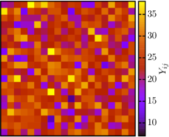
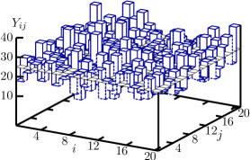
Figure 1: Counts map of a realization of a homogeneous Poisson process (left) and visualization of the threshold procedure (right)

In dependence of a threshold parameter $c\in\mathbb{N}$, we introduce a random $(m+2)\times(m+2)$-matrix $Z=(Z_{i,j})_{i,j=0,\ldots,m+1}$, which is called the digital or binary image. Here,

$$Z_{i,j}=Z_{i,j}^{(m)}(c):=\mathbf{1}\{Y_{i,j}^{(m)}\geq c\}\quad\mbox{if }i,j\in\{1,\ldots,m\}$$

and $Z_{0,j}=Z_{m+1,j}=Z_{i,0}=Z_{i,m+1}=0$ for $i,j=1,\ldots,m$. If we color a cell $C_{i,j}^{(m)}$ black or white according to whether $Z_{i,j}=1$ or $Z_{i,j}=0$, we obtain a binary (black and white) image, as given in Figure 2. Notice that, by definition, there is a white border around the cells $C_{i,j}^{(m)}$, $1\leq i,j\leq m$, which is needed for the sake of comparability of the Minkowski functionals. The concept of binary images has wide applications in computer science and image analysis, see Klette and Rosenfeld, (2004); Kong and Rosenfeld, (1996). In this respect, many algorithmic tools have been developed which are useful in simulations, see for instance Legland et al., (2007).

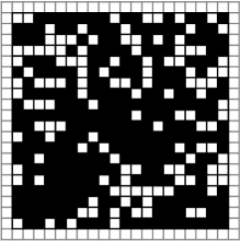
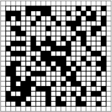
Figure 2: Two binary images of an underlying homogeneous Poisson process for different threshold parameters $c$ (left $c=23$, right $c=27$) and fixed cell number parameter $m=20$

3 Minkowski Functionals and Local Dependency

The main idea underlying the new tests of CSR is to evaluate the resulting binary image by means of geometric functionals. In the bivariate case, there are three Minkowski functionals, namely the area, the perimeter, and the Euler characteristic. Knowledge of the values of these functionals does not characterize the binary image. Nevertheless, Hadwiger’s characterization theorem states that every functional acting on nonempty compact convex subsets of $\mathbb{R}^{d}$, $d\in\mathbb{N}$, that is additive, continuous and invariant under rigid motions can be written as a linear combination of the Minkowski functionals, for details see Schneider and Weil, (2008), p. 628.

A natural question is: Given a $m\times m$ binary image with white border, how can these functionals be computed in an efficient way? Obviously, we can calculate the area by simply counting the black cells, but the answer for the other functionals is more involved. However, results from image analysis allow to establish a look-up table like Table 1 (even in higher dimensions), see Gray, (1971); Mantz et al., (2008); Mecke, K. and Stoyan, D. , 2000 (Eds.) for early versions in two dimensions and Kong and Rosenfeld, (1989) for a survey.

Table 1: Look-up table for Minkowski functionals: the functional values of the area $A$, the perimeter $P$, and the Euler characteristic $\chi$ are assigned to each $2\times 2$-combination of pixels. The unit of length is the edge-length of a pixel.

Configuration		$A$	$P$	$\chi$	Configuration		$A$	$P$	$\chi$
1		0	0	0	9		1/4	1	1/4
2		1/4	1	1/4	10		1/2	2	-1/2
3		1/4	1	1/4	11		1/2	1	0
4		1/2	1	0	12		3/4	1	-1/4
5		1/4	1	1/4	13		1/2	1	0
6		1/2	1	0	14		3/4	1	-1/4
7		1/2	2	-1/2	15		3/4	1	-1/4
8		3/4	1	-1/4	16		1	0	0

Here, we move a small $(2\times 2)$-window over the whole digital image (from top left to bottom right) and sum up the values given in the table according to the observed configuration. A basic feature of the structure underlying the look-up table is that each cell can only have an effect on the 8 neighboring cells, which implies a local dependency structure. Given a random digital image $Z$, we thus define

$$A_{m,c}:=\frac{1}{m}\sum_{i,j=1}^{m}Z_{i,j}$$ (3)

as the (scaled) total area covered by ’non-border’ cells, the counts of which exceed the threshold $c$, and the perimeter

$$P_{m,c}:=\frac{1}{m}\sum_{i,j=1}^{m}\psi(Z_{i,j}),$$ (4)

where, for $i,j\in\{1,\ldots,m\}$,

$$\psi(Z_{i,j}):=\left\{\begin{array}[]{cc}0,&\mbox{if}\;Z_{i,j}=0,\\ 4-(Z_{i-1,j}+Z_{i+1,j}+Z_{i,j-1}+Z_{i,j+1}),&\mbox{if}\;Z_{i,j}=1.\end{array}\right.$$

Motivated by look-up Table 1, we finally study the (scaled) Euler characteristic

$$\chi_{m,c}:=\frac{1}{m}\sum_{i,j=1}^{m}W_{i,j},$$ (5)

where, putting $S_{i,j}:=Z_{i,j}+Z_{i+1,j}+Z_{i,j+1}+Z_{i+1,j+1}$,

$$W_{i,j}:=\left\{\begin{array}[]{ll}1/4,&\text{ if }S_{i,j}=1,\\ -1/4,&\text{ if }S_{i,j}=3,\\ -1/2,&\text{ if }S_{i,j}=2\text{ and }Z_{i,j}Z_{i+1,j+1}=1\text{ or }Z_{i+1,j}Z_{i,j+1}=1,\\ 0,&\text{ otherwise }.\end{array}\right.$$ (6)

Each of these functionals is a sum of random variables that depend on the color of the cells $C_{i,j}^{(m)}$. Notice that the summands figuring in (4) and (5) are neither independent nor identically distributed.

In view of the $(2\times 2)$ observation window that is moved over the binary picture, one can compute each functional as a weighted sum of indicators. As an example, the product

$$(1-Z_{i,j})(1-Z_{i,j+1})(1-Z_{i+1,j})Z_{i+1,j+1}$$

is the indicator of the occurrence of configuration 2 of the look-up Table 1 at (top left bin) position $(i,j)$. Implementing the look-up table and summing up over all positions with the appropriate weights, one obtains an alternative representation of each of the functionals. For instance, the (scaled) Euler characteristic takes the form

$$\chi_{m,c} = \frac{1}{m}\sum_{i,j=1}^{m}\frac{1}{4}\left(Z_{i,j}^{(m)}+Z_{i,j+1}^{(m)}+Z_{i+1,j}^{(m)}+Z_{i+1,j+1}^{(m)}\right)$$ (7)

$$-\frac{1}{2}\left(Z_{i,j}^{(m)}Z_{i+1,j}^{(m)}+Z_{i,j}^{(m)}Z_{i,j+1}^{(m)}+Z_{i,j+1}^{(m)}Z_{i+1,j+1}^{(m)}+Z_{i+1,j}^{(m)}Z_{i+1,j+1}^{(m)}\right.$$

$$\left.+2Z_{i,j}^{(m)}Z_{i+1,j+1}^{(m)}+2Z_{i,j+1}^{(m)}Z_{i+1,j}^{(m)}\right)+Z_{i,j}^{(m)}Z_{i,j+1}^{(m)}Z_{i+1,j}^{(m)}$$

$$+Z_{i,j}^{(m)}Z_{i,j+1}^{(m)}Z_{i+1,j+1}^{(m)}+Z_{i,j}^{(m)}Z_{i+1,j}^{(m)}Z_{i+1,j+1}^{(m)}+Z_{i,j+1}^{(m)}Z_{i+1,j}^{(m)}Z_{i+1,j+1}^{(m)}$$

$$-Z_{i,j}^{(m)}Z_{i,j+1}^{(m)}Z_{i+1,j}^{(m)}Z_{i+1,j+1}^{(m)}.$$

This representation will be used in the proof of Theorem 7.3.

4 Mean and Variance under $H_{0}$

To establish a test statistic for CSR we need some characteristics like the mean, the variance and the covariance of the Minkowski functionals under the hypothesis $H_{0}$. In case of CSR the random variable $Z_{i,j}$ follows the binomial distribution $\mbox{Bin}(1,p_{c})$ where $p_{c}=\mathbb{P}(Z_{i,j}=1)=\mathbb{P}(Y_{i,j}\geq c)$, depends on the underlying known intensity $\lambda$ of ${\cal P}_{\lambda}$ and the threshold $c$. Under $H_{0}$, we have

$$p_{c}:=p_{c}(\lambda,m)=\sum_{k=c}^{\infty}\exp\left(-\frac{\lambda}{m^{2}}\right)\frac{(\lambda/m^{2})^{k}}{k!}=1-\exp\left(-\frac{\lambda}{m^{2}}\right)\sum_{k=0}^{c-1}\frac{(\lambda/m^{2})^{k}}{k!}.$$ (8)

Clearly, if the parameter $\lambda$ is unknown, we will have to estimate it with a good estimator. The natural way to estimate the intensity of a stationary planar Poisson process is to count the number of points falling into an observation window, and to divide this number by the area of the window which, in our case, is one. For more information on estimation techniques see for instance Gaetan and Guyon, (2010), section 5.5.2.1, or for newer developments Coeurjolly, (2017) and the references therein. By the extreme independence property of homogeneous Poisson processes, the $Z_{i,j}$, $i,j=1,\ldots,m$, are independent, and it follows that

$$\sum_{i,j=1}^{m}Z_{i,j}\stackrel{{\scriptstyle\mbox{\scriptsize${\cal D}$}}}{{=}}\mbox{Bin}(m^{2},p_{c}),$$

where ”$\stackrel{{\scriptstyle\mbox{\scriptsize${\cal D}$}}}{{=}}$” means equality in distribution. Thus, the expected (scaled) total area covered by non-border cells is given by

$$\mu_{A}(p_{c}):=\mathbb{E}\left[A_{m,c}\right]=\frac{1}{m}\sum_{i,j=1}^{m}\mathbb{E}\left[Z_{i,j}\right]=mp_{c}.$$

Taking into account the boundary effects, we have

$$\mathbb{E}\left[\psi(Z_{i,j})\right]=\left\{\begin{array}[]{cl}p_{c}(4-4p_{c}),&\mbox{if}\;i,j\in\{2,\ldots,m-1\},\\ p_{c}(4-3p_{c}),&\mbox{if}\;i\in\{1,m\},j\in\{2,\ldots,m-1\},\\ p_{c}(4-3p_{c}),&\mbox{if}\;j\in\{1,m\},i\in\{2,\ldots,m-1\},\\ p_{c}(4-2p_{c}),&\mbox{if}\;i,j\in\{1,m\},\end{array}\right.$$

and the expected perimeter is given by

$$\mu_{P}(p_{c}):=\mathbb{E}\left[P_{m,c}\right]=\frac{1}{m}\sum_{i,j=1}^{m}\mathbb{E}\left[\psi(Z_{i,j})\right]=4p_{c}(m-(m-1)p_{c}).$$

Moreover, the expected Euler characteristic is

$$\mu_{\chi}(p_{c}) := \mathbb{E}\left[\chi_{m,c}\right]=\frac{1}{m}\sum_{i,j=1}^{m}\mathbb{E}\left[W_{ij}\right]$$

$$= \frac{1}{m}\left(p_{c}+2(m-1)p_{c}(1-p_{c})+(m-1)^{2}p_{c}(1-p_{c})(p_{c}^{2}-3p_{c}+1)\right).$$

Thus, each of the mean values of the Minkowski functionals is a function of the probability $p_{c}$, which in turns depends on $m$, the intensity $\lambda$, and the threshold parameter $c$. The variances are given in the next theorem.

Theorem 4.1

Under $H_{0}$ we have

$$\sigma^{2}_{A}:=\mathbb{V}(A_{m,c}) = p_{c}(1-p_{c}),$$

$$\sigma^{2}_{P}:=\mathbb{V}(P_{m,c}) = \frac{8}{m^{2}}p_{c}(1-p_{c})\left((7m^{2}-13m+4)p_{c}^{2}-7m(m-1)p_{c}+2m^{2}\right),$$

$$\sigma^{2}_{\chi}:=\mathbb{V}(\chi_{m,c}) = \frac{1}{m^{2}}p_{c}(1-p_{c})\Big{\{}\left(9m^{2}-30m+25\right)p_{c}^{6}-\left(59m^{2}-194m+159\right)p_{c}^{5}$$

$$+\left(137m^{2}-434m+341\right)p_{c}^{4}-\left(139m^{2}-406m+291\right)p_{c}^{3}$$

$$+\left(64m^{2}-158m+94\right)p_{c}^{2}-\left(12m^{2}-18m+6\right)p_{c}+m^{2}\Big{\}}.$$

Proof: Since the method of computation is the same for each of these formulas, we only illustrate the reasoning by computing $\sigma^{2}_{P}$. To this end, observe that the perimeter can alternatively be written as

$$P_{m,c}=\frac{1}{m}\sum_{i,j=1}^{m}V_{i,j},$$ (9)

where, putting $S_{i,j}:=Z_{i,j}+Z_{i+1,j}+Z_{i,j+1}+Z_{i+1,j+1}$ and invoking Table 1,

$$V_{i,j}:=\left\{\begin{array}[]{ll}1,&\text{ if }S_{i,j}\in\{1,3\},\\ 2,&\text{ if }S_{i,j}=2\text{ and }Z_{i,j}Z_{i+1,j+1}=1\text{ or }Z_{i+1,j}Z_{i,j+1}=1,\\ 0,&\text{ otherwise}.\end{array}\right.$$ (10)

Notice that $V_{i,j}$ assigns one of the values $0,1$ or $2$ to each $(2\times 2)$-window, where the upper left bin is at position $(i,j)$ in the binary picture. We have

$$\mathbb{V}(P_{m,c})=\frac{1}{m^{2}}\left(\sum_{i,j=1}^{m}\mathbb{V}(V_{i,j})+\sum_{\tiny\begin{array}[]{c}i,j,k,\ell=1\\ (i,j)\not=(k,\ell)\end{array}}^{m+1}\mbox{Cov}(V_{i,j},V_{k,\ell})\right).$$

To compute the sum of the variances, observe that

$$\mathbb{V}(V_{1,1}) = p_{c}(1-p_{c}),$$

$$\mathbb{V}(V_{1,2}) = p_{c}(2-p_{c})(1-p_{c}(2-p_{c})),$$

$$\mathbb{V}(V_{2,2}) = 4p_{c}(1-p_{c})(3p_{c}^{2}-3p_{c}+1).$$

By symmetry, we have

$$\sum_{i,j=1}^{m}\mathbb{V}(V_{i,j})=4\mathbb{V}(V_{1,1})+4(m-1)\mathbb{V}(V_{1,2})+(m-1)^{2}\mathbb{V}(V_{2,2}).$$

The computation of the sum of covariances uses the methods presented in the proof of Theorem 6.1. Summing everything up and simplifying the results leads to the stated formulas. $\square$

5 Testing procedures and $H_{0}$-asymptotics

In view of the previous sections a natural way to define the new tests is to standardize the data driven Minkowski functionals under $H_{0}$ in dependence of a fixed threshold parameter $c$. We thus propose

$$T_{A}(c;X_{1},\ldots,X_{N_{\lambda}}) = \frac{1}{\sigma_{A}}\left(A_{m,c}-\mu_{A}(p_{c})\right)^{2},$$ (11)

$$T_{P}(c;X_{1},\ldots,X_{N_{\lambda}}) = \frac{1}{\sigma_{P}}\left(P_{m,c}-\mu_{P}(p_{c})\right)^{2},$$ (12)

$$T_{\chi}(c;X_{1},\ldots,X_{N_{\lambda}}) = \frac{1}{\sigma_{\chi}}\left(\chi_{m,c}-\mu_{\chi}(p_{c})\right)^{2}.$$ (13)

Observe that the variances given in Theorem 4.1 and the probability $p_{c}$ depend on $c$, $m$ and $\lambda$. Rejection of $H_{0}$ is for large values of $T_{A},T_{P}$ or $T_{\chi}$. For the sake of simplicity we assume that $\lambda$ is known, perhaps on the basis of previous experiments. If $\lambda$ has to be estimated, the method of estimation will have effects on the asymptotic statements derived below, as pointed out in Heinrich, (2015). Throughout this section we assume that $H_{0}$ holds. To derive the limits in distribution of the Minkowski functionals we consider the limiting regime

$$\lambda\rightarrow\infty,\,m\rightarrow\infty,\,\frac{\lambda}{m^{2}}\rightarrow\kappa$$ (14)

for some $\kappa\in(0,\infty)$. Under this regime, $\lim\mathbb{E}\left[Y_{i,j}\right]=\kappa$ for each pair $(i,j)$ and the probability $p_{c}=p_{c}(\lambda,m)$ figuring in (8) converges to

$$p_{c}(\kappa)=1-\textrm{e}^{-\kappa}\sum_{k=0}^{c-1}\frac{\kappa^{k}}{k!},$$ (15)

where $0<p_{c}(\kappa)<1$. By the central limit theorem we obviously have

$$\mathcal{A}_{m,\lambda}(c):=\frac{1}{\sigma_{A}}\left(A_{m,c}-\mu_{A}(p_{c})\right)\stackrel{{\scriptstyle\mathcal{D}}}{{\longrightarrow}}\mbox{N}(0,1)$$

under (14), where the symbol $\stackrel{{\scriptstyle\mathcal{D}}}{{\longrightarrow}}$ means convergence in distribution of random variables and vectors. If $c=1$ and $m$ is fixed, the test based on $A_{m,1}$ is related to the empty boxes test, see Viktorova and Chistyakov, (1966) if $\mathbb{P}(N_{\lambda}=n)=1$. Notice that, by the multivariate central limit theorem, we have the convergence in distribution of $(\mathcal{A}_{m,\lambda}(c_{1}),\ldots,\mathcal{A}_{m,\lambda}(c_{s}))^{\prime}$ to some centred $s$-variate normal distribution, for any choice of $s\geq 2$ and $c_{1},\ldots,c_{s}>0$. Thus, in any conceivable space of random sequences, there is convergence of finite-dimensional distributions of a random element ${\cal A}_{m,\lambda}$. However, at least for the separable Banach space of sequences converging to zero, equipped with the supremum norm, the double sequence $({\cal A}_{m,\lambda})_{m,\lambda\geq 1}$, where the limit is taken in respect of the limiting regime (14), is not tight.

Because of the local geometric dependence of the random variables defining the perimeter and the Euler characteristic, we use tools from random geometric graphs, as stated in Penrose, (2004). Let $(I,E)$ be a graph with finite or countable vertex set $I$. For $i,j\in I$, write $i\sim j$ if $\{i,j\}\in E$, where $E$ is the set of edges. For $i\in I$, let ${\cal N}_{i}:=\{i\}\cup\{j\in I:j\sim i\}$ be the so-called adjacency neighbourhood of $i$. The graph $(I,\sim)$ is called an dependency graph for a collection of random variables $(\xi_{i},i\in I)$, if for any disjoint subsets $I_{1},I_{2}$ of $I$ such that there are no edges connecting $I_{1}$ and $I_{2}$, the collection of random variables $(\xi_{i},i\in I_{1})$ is independent of $(\xi_{i},i\in I_{2})$. The following result (Penrose, (2004), Theorem 2.4), plays a central role in proving the next two statements.

Proposition 5.1

Suppose $(\xi_{i})_{i\in I}$ is a finite collection of random variables with dependency graph $(I,\sim)$ having maximum degree $D-1$, where $\mathbb{E}(\xi_{i})=0$ for each $i$. Set $W:=\sum_{i\in I}\xi_{i}$, and suppose $\mathbb{E}(W^{2})=1$. Then

$$\sup_{t\in\mathbb{R}}|\mathbb{P}(W\leq t)-\Phi(t)|\leq\frac{2}{(2\pi)^{1/4}}\sqrt{D^{2}\sum_{i\in I}\mathbb{E}|\xi_{i}|^{3}}+6\sqrt{D^{3}\sum_{i\in I}\mathbb{E}|\xi_{i}|^{4}},$$

where $\Phi$ is the distribution function of a standard normal distribution N$(0,1)$.

The next result concerns the perimeter $P_{m,c}$.

Theorem 5.2

For each fixed $c\in\mathbb{N}$ we have under the limiting regime (14)

$$\frac{1}{\sigma_{P}}\left(P_{m,c}-\mu_{P}(p_{c})\right)\stackrel{{\scriptstyle\mathcal{D}}}{{\longrightarrow}}{\rm{N}}(0,1).$$

Proof: In view of Theorem 5.1 we choose the vertex set

$$I:=\{i:=(i_{1},i_{2},i_{1}-1,i_{1}+1,i_{2}-1,i_{2}+1):(i_{1},i_{2})\in\{1,\ldots,m\}^{2}\}$$

and define

$$\xi_{i}:=\frac{1}{m\sigma_{P}}\left(\psi(Z_{i_{1},i_{2}})-\mathbb{E}\left[\psi(Z_{i_{1},i_{2}})\right]\right),\quad i\in I.$$ (16)

Then $\mathbb{E}(\xi_{i})=0$ and $\mathbb{E}\left|\psi(Z_{i_{1},i_{2}})-\mathbb{E}\left[\psi(Z_{i_{1},i_{2}})\right]\right|^{\ell}<\infty$ if $\ell\in\{3,4\}$ and thus

$$\mathbb{E}|\xi_{i}|^{\ell}=(m\sigma_{P})^{-\ell}O(1).$$

To construct a dependency graph we write $i\sim j:\Longleftrightarrow|j_{1}-i_{1}|+|j_{2}-i_{2}|\leq 2$ if $i\in I$ is as above and $j:=(j_{1},j_{2},j_{1}-1,j_{1}+1,j_{2}-1,j_{2}+1)\in I$. Notice that ${\cal N}_{i}$ has at most 13 elements, which shows that, in our case, the constant $D$ figuring in the statement of Theorem 5.1 is $13$. With this notation we have

$$W:=\sum_{i\in I}\xi_{i}=\frac{1}{\sigma_{P}}\left(P_{m,c}-\mathbb{E}(P_{m,c})\right).$$

Therefore, since $\sigma_{P}^{2}\rightarrow 8p_{c}(\kappa)(1-p_{c}(\kappa))\left(7p_{c}(\kappa)^{2}-7p_{c}(\kappa)+2\right)$ under the limiting regime (14), putting $D=13$ and invoking Proposition 5.1 yields

$$\sup_{t\in\mathbb{R}}|\mathbb{P}(W\leq t)-\Phi(t)| \leq \frac{2}{(2\pi)^{1/4}}\sqrt{D^{2}\sum_{i\in I}\mathbb{E}|\xi_{i}|^{3}}+6\sqrt{D^{3}\sum_{i\in I}\mathbb{E}|\xi_{i}|^{4}}$$

$$= \frac{2D}{(2\pi)^{1/4}\sqrt{m\sigma_{P}^{3}}}O(1)+\frac{6\sqrt{D^{3}}}{m\sigma_{P}^{2}}O(1)\rightarrow 0.$$

$\square$
To handle the Euler characteristic, take

$$I:=\{i=(i_{1},i_{2},i_{1}+1,i_{2}+1):(i_{1},i_{2})\in\{1,\ldots,m\}^{2}\}$$

and for $i\in I$, put $S_{i}:=Z_{i_{1},i_{2}}+Z_{i_{1},i_{2}+1}+Z_{i_{1}+1,i_{2}}+Z_{i_{1}+1,i_{2}+1}$. In this case, with $i$ as above and $j=(j_{1},j_{2},j_{1}+1,j_{2}+1)\in I$, we construct a dependency graph via

$$i\sim j:\Longleftrightarrow\max(|i_{1}-j_{1}|,|i_{2}-j_{2}|)\leq 1.$$

Theorem 5.3

Under the limiting regime (14), we have

$$\frac{1}{\sigma_{\chi}}\left(\chi_{m,c}-\mu_{\chi}(p_{c})\right)\stackrel{{\scriptstyle\mathcal{D}}}{{\longrightarrow}}\mbox{\rm N}(0,1)$$

for each fixed $c\in\mathbb{N}$.

Proof: With the dependency graph given above, the proof parallels that of Theorem 5.2, upon noting that, with

$$\xi_{i}^{*}:=\frac{W_{i}-\mathbb{E}\left[W_{i}\right]}{m\sigma_{\chi}},$$

we have $\mathbb{E}\left[|\xi_{i}^{*}|^{\ell}\right]=O((m\sigma_{\chi})^{-\ell})$. $\square$

The continuous mapping theorem now yields the following result.

Corollary 5.4

For fixed $c\in\mathbb{N}$, we have under the limiting regime (14)

$$T_{j}(c;X_{1},\ldots,X_{N_{\lambda}})\stackrel{{\scriptstyle\mathcal{D}}}{{\longrightarrow}}\chi^{2}_{1},\quad j\in\{A,P,\chi\}.$$

6 Combinations of more than one functional

On the basis of promising results regarding the power of tests of $H_{0}$ against specific alternatives (see Section 8), we also considered test statistics that make use of more than one of the Minkowski functionals. Such an approach requires knowledge of the covariances $\sigma_{A,P}:=\mbox{Cov}(A_{m,c},P_{m,c})$, $\sigma_{A,\chi}:=\mbox{Cov}(A_{m,c},\chi_{m,c})$ and $\sigma_{P,\chi}:=\mbox{Cov}(P_{m,c},\chi_{m,c})$. These are given as follows.

Theorem 6.1

Under $H_{0}$ we have

$$\sigma_{A,P} = \frac{1}{m^{2}}p_{c}(1-p_{c})(4m^{2}(1-2p_{c})+8mp_{c}),$$

$$\sigma_{A,\chi} = \frac{1}{m^{2}}p_{c}(1\!-\!p_{c})\left(-4(m\!-\!1)^{2}p_{c}^{3}+12(m\!-\!1)^{2}p_{c}^{2}-4(m\!-\!1)(2m\!-\!1)p_{c}+m^{2}\right),$$

$$\sigma_{P,\chi} = \frac{4}{m^{2}}p_{c}(1-p_{c})\Big{\{}\left(6m^{2}-16m+10\right)p_{c}^{4}-\left(22m^{2}-56m+34\right)p_{c}^{3}$$

$$+\left(23m^{2}-49m+24\right)p_{c}^{2}-\left(9m^{2}-13m+4\right)p_{c}+m^{2}\Big{\}}.$$

Proof: Since the proof is involved due to messy computations, we only show how to compute $\sigma_{P,\chi}$ for the case $m\geq 3$. The other covariances are tackled in a similar fashion. From (5) and (9), we have

$$\sigma_{P,\chi}=\frac{1}{m^{2}}\sum_{i,j,k,\ell=1}^{m}\mbox{Cov}(V_{i,j},W_{k,\ell}),$$

where $V_{i,j}$ and $W_{i,j}$ are given in (10) and (6), respectively. Notice that, due to the underlying local dependence structure, the covariance $\mbox{Cov}(V_{i,j},W_{k,\ell})$ vanishes for each pair $(i,j)$ and $(k,\ell)$ of cells that are not neighbors in the sense that at least one bin of the respective $(2\times 2)$-windows overlaps. For neighboring cells, the resulting covariance depends on how the two cells overlap, giving rise to different ’covariance configurations’. To compute the covariances we have to address the following questions.

• How many different types of covariance configurations appear in the sum?

• What are the formulae for the different covariance configurations?

• How often do we have to count each covariance configuration?

As for the first question, observe that, due to the white border of the observation window (see Figure 2) and the presence of neighboring cells that have joint bins with the border, we have to distinguish the 7 cases ’corners’, ’side-corners’, ’borders’, ’inner-corners’, ’inner-side-corners’, ’inner-borders’ and ’middle cells’: Each of theses cases gives rise to a separate covariance configuration. In the same order, the answer to the third question for these configurations is $4,8,4(m-3),4,8,4(m-3),(m-3)^{2}$. As an example, we compute the covariance formula for two special cases, namely ’corner’ and ’side-corner’. For the case ’corner’, fixing $V_{1,1}$ and invoking a symmetry argument gives

$$\mbox{Cov}(V_{1,1},W_{1,1})+2\mbox{Cov}(V_{1,1},W_{1,2})+\mbox{Cov}(V_{1,1},W_{2,2}),$$ (17)

since the upper left $(2\times 2)$-window has four neighboring $(2\times 2)$-windows with intersecting bins. Since, under $H_{0}$, the colorings of the single bins are independent, the summands above read

$$\mbox{Cov}(V_{1,1},W_{1,1})=\frac{1}{4}p_{c}(1-p_{c}),\quad\mbox{Cov}(V_{1,1},W_{1,2})=\frac{1}{4}p_{c}(1-p_{c})(1-2p_{c}),$$

and

$$\mbox{Cov}(V_{1,1},W_{2,2})=-\frac{1}{4}p_{c}(1-p_{c})(4p_{c}^{3}-12p_{c}^{2}+8p_{c}-1).$$

Thus, the sum figuring in (17) equals $p_{c}(1-p_{c})^{4}$, which is the contribution to the total covariance of each of the corners. For the case ’side-corner’ we fix $V_{1,2}$ and, again due to symmetry, have to consider five summands, namely

$$\mbox{Cov}(V_{1,2},W_{1,1})+\mbox{Cov}(V_{1,2},W_{1,2})+2\mbox{Cov}(V_{1,2},W_{1,3})$$

$$+\mbox{Cov}(V_{1,2},W_{2,2})+\mbox{Cov}(V_{1,2},W_{2,3}).$$

Calculation of each summand and summing up gives the contribution $p_{c}(1-2p_{c})(2-p_{c})(1-p_{c})^{3}$ to the total covariance for each ’side-corner’-case of pairs of cells. Counting the number of times that each of the different configurations that yield a non-vanishing contribution to the total covariance can occur and summing up, the final result follows from tedious calculations. $\square$

The formulas figuring in Theorem 6.1 have been simplified using the CAS Maple 18, and they have been checked by Monte Carlo simulations in R. The complete covariance structure between the Minkowski functionals is given by the symmetric ($3\times 3$)-matrix

$$\Sigma_{c,m,\lambda}:=\left(\begin{array}[]{ccc}\sigma^{2}_{A}&\sigma_{A,P}&\sigma_{A,\chi}\\ \sigma_{A,P}&\sigma^{2}_{P}&\sigma_{P,\chi}\\ \sigma_{A,\chi}&\sigma_{P,\chi}&\sigma^{2}_{\chi}\end{array}\right).$$

The index stresses the dependence of the covariance structure on the threshold parameter $c$, the underlying intensity $\lambda$ of the PPP, and on $m$. The determinant of $\Sigma_{c,m,\lambda}$ is given by

$$\det\left(\Sigma_{c,m,\lambda}\right) = \frac{8}{m^{6}}p_{c}^{5}(1-p_{c})^{3}\Big{\{}-(m^{2}-3m+4)^{3}p_{c}^{6}$$

$$+2(2m^{2}-5m+6)(m^{2}-3m+4)(m^{2}-5m+8)p_{c}^{5}$$

$$+(-4m^{6}+50m^{5}-280m^{4}+878m^{3}-1580m^{2}+1552m-704)p_{c}^{4}$$

$$+(-4m^{6}+22m^{5}-302m^{3}+828m^{2}-880m+384)p_{c}^{3}$$

$$+\left(11m^{6}-77m^{5}+229m^{4}-275m^{3}+56m^{2}+112m-64\right)p_{c}^{2}$$

$$-4m(m-1)(2m^{4}-9m^{3}+20m^{2}-18m+4)p_{c}+2m^{3}(m-1)^{3}\Big{\}}.$$

According to Maple 18, there is an explicit representation of the inverse of $\Sigma_{c,m,\lambda}$, which shows that for $0<p_{c}<1$ the matrix $\Sigma_{c,m,\lambda}$ is nonsingular for each $p_{c}\in(0,1)$. This expression, however, is too complicated to be reproduced here. Letting $m\rightarrow\infty$ we obtain the asymptotic covariance matrix

$$\Sigma := p_{c}(1-p_{c})\left\{\mbox{diag}(0,0,9)p_{c}^{6}+\mbox{diag}(0,0,-59)p_{c}^{5}+\left(\begin{array}[]{ccc}0&0&0\\ 0&0&24\\ 0&24&137\end{array}\right)p_{c}^{4}\right.$$

$$\left.+\left(\begin{array}[]{ccc}0&0&-4\\ 0&0&-88\\ -4&-88&-139\end{array}\right)p_{c}^{3}+\left(\begin{array}[]{ccc}0&0&12\\ 0&56&92\\ 12&92&64\end{array}\right)p_{c}^{2}+\left(\begin{array}[]{ccc}0&-8&-4\\ -8&-56&-36\\ -4&-36&-12\end{array}\right)p_{c}\right.$$

$$\left.+\left(\begin{array}[]{ccc}1&4&1\\ 4&16&4\\ 1&4&1\end{array}\right)\right\}.$$

This is nonsingular if $0<p_{c}<1$, since the inverse matrix is given by

$$\Sigma^{-1} := \left(p_{c}^{2}(1-p_{c})^{4}(p_{c}^{2}-2)\right)^{-1}\cdot\left\{\mbox{diag}(-9,0,0)p_{c}^{6}\right.$$

$$\left.+\left(\begin{array}[]{ccc}43&-3&0\\ -3&0&0\\ 0&0&0\end{array}\right)p_{c}^{5}+\left(\begin{array}[]{ccc}-87&27/2&0\\ 27/2&-7/8&0\\ 0&0&0\end{array}\right)p_{c}^{4}+\left(\begin{array}[]{ccc}103&-22&4\\ -22&15/4&0\\ 4&0&0\end{array}\right)p_{c}^{3}\right.$$

$$\left.+\left(\begin{array}[]{ccc}-76&35/2&-8\\ 35/2&-41/8&1\\ -8&1&0\end{array}\right)p_{c}^{2}+\left(\begin{array}[]{ccc}30&-8&4\\ -8&5/2&-2\\ 4&-2&0\end{array}\right)p_{c}+\left(\begin{array}[]{ccc}-5&3/2&-1\\ 3/2&-1/2&1/2\\ -1&1/2&-1\end{array}\right)\right\}.$$

Since the mean, the variance, and the covariance structure have been computed under $H_{0}$, one may expect that, for each value of the threshold parameter $c$, the standardized vector

$$\Sigma_{c,m,\lambda}^{-\frac{1}{2}}\left(\left(A_{m,c},P_{m,c},\chi_{m,c}\right)^{\top}-\mu_{c}\right)$$

does not deviate too much from the origin in $\mathbb{R}^{3}$. Here, $\Sigma_{c,m,\lambda}^{-\frac{1}{2}}$ denotes the symmetric square root of $\Sigma_{c,m,\lambda}^{-1}$, $\top$ stands for the transposition of vectors and matrices, and $\mu_{c}:=(\mu_{A},\mu_{P},\mu_{\chi})^{\top}$. Writing $\|\cdot\|$ for the Euclidean norm, we define a family of test statistics depending on $c$, namely

$$T_{c}(X_{1},\ldots,X_{N_{\lambda}}) := \left\|\Sigma_{c,m,\lambda}^{-\frac{1}{2}}\left(\left(A_{m,c},P_{m,c},\chi_{m,c}\right)^{\top}-\mu_{c}\right)\right\|^{2}$$

$$= \left(\!\left(A_{m,c},P_{m,c},\chi_{m,c}\right)^{\top}\!-\!\mu_{c}\right)^{\top}\Sigma_{c,m,\lambda}^{-1}\left(\!\left(A_{m,c},P_{m,c},\chi_{m,c}\right)^{\top}\!-\!\mu_{c}\right).$$

An asymptotic equivalent alternative to this statistic is

$$\widetilde{T}_{c}(X_{1},\ldots,X_{N_{\lambda}}):=\left(\left(A_{m,c},P_{m,c},\chi_{m,c}\right)^{\top}-\mu_{c}\right)^{\top}\Sigma^{-1}\left(\left(A_{m,c},P_{m,c},\chi_{m,c}\right)^{\top}-\mu_{c}\right).$$

Rejection of $H_{0}$ is for large values of $T_{c}$ or $\widetilde{T}_{c}$.

In what follows, we state the asymptotic distributions of $T_{c}$ and $\widetilde{T}_{c}$ under $H_{0}$. As in Section 5 our main problem is the local dependency structure of the vector $(A_{m,c},P_{m,c},\chi_{m,c})$.

Theorem 6.2

Under the limiting regime (14), we have for fixed $c\in\mathbb{N}$

1. $T_{c}\stackrel{{\scriptstyle\mathcal{D}}}{{\longrightarrow}}\chi^{2}_{3}$,
   

2. $\widetilde{T}_{c}\stackrel{{\scriptstyle\mathcal{D}}}{{\longrightarrow}}\chi^{2}_{3}$.

Proof: We use Theorem 2.2 of Rinott and Rotar, (1996). To this end, fix $(i,j)\in\{1,\ldots,m\}^{2}$, and let $S_{(i,j)}$ be the set of indices of the points that are neighbors of $(i,j)$, enlarged by $\{(i,j)\}$. Moreover, put $\displaystyle\mathcal{N}_{(i,j)}=\textstyle{\bigcup_{(k,\ell)\in S_{(i,j)}}}S_{(k,\ell)}$. The set $S_{(i,j)}$ has at most 9 elements, and the cardinality of ${\cal N}_{(i,j)}$ is at most 81. Arguing as in the example on p. 338 of Rinott and Rotar, (1996), we see that each of the constants $\chi_{1},\chi_{2},\chi_{3}$ figuring in formula (2.2) of Rinott and Rotar, (1996) vanishes. Suppose $\mathcal{H}$ is a class of measurable functions from $\mathbb{R}^{3}$ to $\mathbb{R}$ which is closed under affine transformation of the argument and satisfies the conditions on p. 335 of Rinott and Rotar, (1996). Theorem 2.2 of Rinott and Rotar, (1996) then states that, for constants $\alpha_{1},\alpha_{2}$ and $\boldmath{W}:=(A_{m,c},P_{m,c},\chi_{m,c})$, we have

$$\sup\{|\mathbb{E}(h(\boldmath{W}))\!-\!\Phi h|:h\!\in\!\mathcal{H}\}\leq 81\alpha_{1}\left(\alpha_{2}B_{m}+9m^{2}\alpha_{2}B_{m}^{3}(|\log B_{m}|+2\log m)\!\right).$$

Here, $B_{m}$ is $o(1/m)$, and $\Phi h=\int_{\mathbb{R}^{3}}h(z)\Phi(dz)$, where $\Phi$ denotes the multivariate standard normal distribution function. From the invariance of affine transformations of $\mathcal{H}$, we therefore have under the limiting regime (14)

$$\Sigma_{c,m,\lambda}^{-\frac{1}{2}}(W-\mathbb{E}(W))\stackrel{{\scriptstyle\mathcal{D}}}{{\longrightarrow}}\textrm{N}_{3}(0,\textrm{I}_{3}),$$

where $\textrm{N}_{3}(0,\textrm{I}_{3})$ denotes a centered three-dimensional normal distribution with unit covariance matrix. Assertion a) then follows from the continuous mapping theorem. Since $\Sigma_{c,m\lambda}\to\Sigma$ under the limiting regime (14), assertion b) is a consequence of a) and Slutzky’s Lemma. $\square$.

7 Asymptotics under alternatives

A feasible alternative could be the following: Let $f$ be a continuous Lebesgue density over $[0,1]^{2}$. Suppose ${\cal P}_{\lambda f}:=\{X_{1},\ldots,X_{N_{\lambda}}\}$ is a Poisson process on $[0,1]^{2}$ with intensity function $\lambda f$, i.e., $(X_{j})_{j\geq 1}$ is a sequence of i.i.d. random variables with density $f$ and $N_{\lambda}\stackrel{{\scriptstyle\mbox{\scriptsize${\cal D}$}}}{{=}}\text{Po}(\lambda)$, independent of $(X_{j})_{j\geq 1}$. For a Borel subset $A$ of $[0,1]^{2}$, let ${\cal P}_{\lambda f}(A):=\sum_{i=1}^{N_{\lambda}}{\bf 1}\{X_{i}\in A\}$ be the number of points of ${\cal P}_{\lambda f}$ in $A$. Then, putting $p_{A}:=\int_{A}f(x)\mbox{d}x$, and conditioning on $N_{\lambda}$, we have ${\cal P}_{\lambda f}(A)\stackrel{{\scriptstyle\mbox{\scriptsize${\cal D}$}}}{{=}}\text{Po}\left(\lambda\int_{A}f(x)\mbox{d}x\right)$. Moreover, for any pairwise disjoint Borel sets $B_{1},\ldots,B_{\ell}$ of $[0,1]^{2}$, the random variables ${\cal P}_{\lambda f}(B_{1}),\ldots,{\cal P}_{\lambda f}(B_{\ell})$ are independent. Let $A_{m,c},P_{m,c}$ and $\chi_{m,c}$ be defined as in (3), (4) and (5), respectively, where, for fixed $c\in\mathbb{N}$, $Z^{(m)}_{i,j}:={\bf 1}\{{\cal P}_{\lambda f}(C^{(m)}_{i,j})\geq c\}$ and $C^{(m)}_{i,j}$ as in (1). Since $f$ is continuous, we have under the limiting regime (14)

$$a_{i,j}^{(m)}:=\lambda\int_{C^{(m)}_{i,j}}f(x)\mbox{d}x\sim\kappa f\left(\frac{i}{m},\frac{j}{m}\right),$$ (23)

where $\sim$ means asymptotic equivalence under the limiting regime. Moreover, since $[0,1]^{2}$ is compact, $f$ is uniformly continuous over $[0,1]^{2}$ by the Heine–Cantor theorem. Writing an unspecified integral for integration over the unit square, and denoting

$$q_{c,\kappa,f}(x):=\sum_{k=0}^{c-1}\frac{\kappa^{k}}{k!}f(x)^{k}{\rm{e}}^{-\kappa f(x)},\quad c\geq 1,\kappa>0,x\in[0,1]^{2},$$ (24)

we have the following result.

Theorem 7.1

Under ${\cal P}_{\lambda f}$ and the limiting regime (14), we have for fixed $c\in\mathbb{N}$

$$\frac{1}{m}A_{m,c}\stackrel{{\scriptstyle\mbox{\small{a.s.}}}}{{\longrightarrow}}1-\int q_{c,\kappa,f}(x){\rm{d}}x.$$

Proof: Invoking (23) we have

$$\mathbb{E}\left[A_{m,c}\right] = \frac{1}{m}\sum_{i,j=1}^{m}\mathbb{P}\left({\cal P}_{\lambda f}\left(C^{(m)}_{i,j}\right)\geq c\right)$$

$$= \frac{1}{m}\sum_{i,j=1}^{m}\left(1-\sum_{k=0}^{c-1}\exp\left(-a^{(m)}_{i,j}\right)\,\frac{1}{k!}\,\left(a^{(m)}_{i,j}\right)^{k}\right)$$

$$= m-\sum_{k=0}^{c-1}\frac{1}{k!}\sum_{i,j=1}^{m}\frac{1}{m}\exp\left(-a^{(m)}_{i,j}\right)\,\left(a^{(m)}_{i,j}\right)^{k},$$

and thus, using the asymptotic equivalence in (23),

$$\lim\mathbb{E}\left(\frac{1}{m}A_{m,c}\right)=1-\sum_{k=0}^{c-1}\frac{\kappa^{k}}{k!}\int f(x)^{k}\mbox{e}^{-\kappa f(x)}\mbox{d}x.$$ (25)

Since $\mathbb{V}(m^{-1}A_{m,c})\leq m^{-2}$, Tschebyshev’s inequality gives

$$\sum_{m=1}^{\infty}\mathbb{P}\left(\frac{1}{m}|A_{m,c}-\mathbb{E}A_{m,c}|\geq\varepsilon\right)<\infty$$

for each positive $\varepsilon$. The lemma of Borel-Cantelli yields $\frac{1}{m}(A_{m,c}-\mathbb{E}A_{m,c})\to 0$ $\mathbb{P}$-a.s. In view of (25), we are done. $\square$

Putting

$$L_{c}(u):=\frac{1}{(c-1)!}\int_{0}^{u}\mbox{e}^{-t}\,t^{c-1}\,\mbox{d}t,\qquad u>0,$$

for $c\in\mathbb{N}$, monotone convergence and a well-known relation between probabilities of level exceedances of Poisson distributions and the lower incomplete Gamma function yield

$$1-\int q_{c,\kappa,f}(x)\mbox{d}x = \int\sum_{k=c}^{\infty}\frac{\kappa^{k}}{k!}f(x)^{k}\mbox{e}^{-\kappa f(x)}\mbox{d}x$$

$$= \int\mathbb{P}\left(\text{Po}(\kappa f(x))\geq c\right)\mbox{d}x$$

$$= \int\frac{1}{(c-1)!}\int_{0}^{\kappa f(x)}\mbox{e}^{-t}t^{c-1}\mbox{d}t\,\mbox{d}x$$

$$= \int L_{c}\left(\kappa f(x)\right)\,\mbox{d}x.$$

If $c=1$, Jensen’s inequality shows that this expression attains its maximum value $1-\mbox{e}^{-\kappa}$ if, and only if, $f$ is the uniform density over $[0,1]^{2}$. Such a result that characterizes the uniform distribution by an extremal property does no longer hold if $c\geq 2$, since, as is readily seen, the function $L_{c}$ is strictly convex on $(0,c-1)$ and strictly concave on $(c,\infty)$. This observation is connected to a two-crossings theorem regarding mixtures from distributions that belong to exponential families, see Shaked, (1980) or Karlis and Xekalaki, (2005), p. 39.

Theorem 7.2

Under ${\cal P}_{\lambda f}$ and the limiting regime (14), we have for fixed $c\in\mathbb{N}$

$$\frac{1}{m}P_{m,c}\stackrel{{\scriptstyle\mbox{\small{a.s.}}}}{{\longrightarrow}}I_{c,\kappa}(f),$$

where

$$I_{c,\kappa}(f):=4\left(\int q_{c,\kappa,f}(x)\mbox{d}x-\int q_{c,\kappa,f}^{2}(x)\mbox{d}x\right).$$

Proof: For the (scaled) perimeter $P_{m,c}$ we have

$$\mathbb{E}\left[P_{m,c}\right]=\frac{1}{m}\sum_{i,j=1}^{m}\mathbb{E}\left(Z_{i,j}^{(m)}\left[4-Z_{i-1,j}^{(m)}-Z_{i+1,j}^{(m)}-Z_{i,j-1}^{(m)}-Z_{i,j+1}^{(m)}\right]\right).$$

By the complete independence property of ${\cal P}_{\lambda f}$,

$$\mathbb{E}\left[Z_{i,j}^{(m)}Z_{i-1,j}^{(m)}\right] = \mathbb{P}\left({\cal P}_{\lambda f}\left(C^{(m)}_{i,j}\right)\geq c,{\cal P}_{\lambda f}\left(C^{(m)}_{i-1,j}\right)\geq c\right)$$

$$= \mathbb{P}\left({\cal P}_{\lambda f}\left(C^{(m)}_{i,j}\right)\geq c\right)\mathbb{P}\left({\cal P}_{\lambda f}\left(C^{(m)}_{i-1,j}\right)\geq c\right),$$

and likewise for $\mathbb{E}\left[Z_{i,j}^{(m)}Z_{i+1,j}^{(m)}\right]$ etc. With $a^{(m)}_{i,j}$ in (23) we have

$$\mathbb{P}\left({\cal P}_{\lambda f}\left(C^{(m)}_{i,j}\right)\geq c\right)=1-\sum_{k=0}^{c-1}\exp\left(-a^{(m)}_{i,j}\right)\,\frac{1}{k!}\,\left(a^{(m)}_{i,j}\right)^{k}$$ (26)

and thus

$$\mathbb{E}\left[Z_{i,j}^{(m)}Z_{i-1,j}^{(m)}\right] = 1\!-\!\sum_{k=0}^{c-1}\!\exp\!\left(\!-a^{(m)}_{i,j}\right)\frac{1}{k!}\left(\!a^{(m)}_{i,j}\!\right)^{k}-\sum_{\ell=0}^{c-1}\!\exp\!\left(\!-a^{(m)}_{i-1,j}\right)\frac{1}{\ell!}\left(\!a^{(m)}_{i-1,j}\!\right)^{\ell}$$

$$\qquad+\sum_{k,\ell=0}^{c-1}\frac{1}{k!\ell!}\exp\left(-a^{(m)}_{i,j}-a^{(m)}_{i-1,j}\right)\left(a^{(m)}_{i,j}\right)^{k}\left(a^{(m)}_{i-1,j}\right)^{\ell}.$$

It follows that

$$\frac{1}{m}\sum_{i,j=1}^{m}\mathbb{E}\left[Z_{i,j}^{(m)}Z_{i-1,j}^{(m)}\right] = m-\sum_{k=0}^{c-1}\frac{1}{k!}\sum_{i,j=1}^{m}\frac{1}{m}\exp\left(-a^{(m)}_{i,j}\right)\left(a^{(m)}_{i,j}\right)^{k}$$

$$\ -\sum_{\ell=0}^{c-1}\frac{1}{\ell!}\sum_{i,j=1}^{m}\frac{1}{m}\exp\!\left(\!-a^{(m)}_{i-1,j}\!\right)\!\left(\!a^{(m)}_{i-1,j}\!\right)^{\ell}$$

$$\ +\sum_{k,\ell=0}^{c-1}\frac{1}{k!\ell!}\sum_{i,j=1}^{m}\frac{1}{m}\!\exp\!\left(\!-a^{(m)}_{i,j}\!-\!a^{(m)}_{i-1,j}\!\right)\left(\!a^{(m)}_{i,j}\!\right)^{k}\!\left(\!a^{(m)}_{i-1,j}\!\right)^{\ell}.$$

In view of (23), the uniform continuity of $f$ and a symmetry argument give

$$\lim\frac{1}{m^{2}}\sum_{i,j=1}^{m}\mathbb{E}\left[Z_{i,j}^{(m)}Z_{i-1,j}^{(m)}\right] = 1-2\sum_{k=0}^{c-1}\frac{\kappa^{k}}{k!}\int\mbox{e}^{-\kappa f(x)}f(x)^{k}\mbox{d}x$$

$$\qquad+\sum_{k,\ell=0}^{c-1}\frac{\kappa^{k+\ell}}{k!\ell!}\int\textrm{e}^{-2\kappa f(x)}f(x)^{k+\ell}\mbox{d}x.$$

The same limits arise if we consider

$$\frac{1}{m^{2}}\sum_{i,j=1}^{m}\mathbb{E}\left[Z_{i,j}^{(m)}Z_{i-1,j}^{(m)}\right],\ \frac{1}{m^{2}}\sum_{i,j=1}^{m}\mathbb{E}\left[Z_{i,j}^{(m)}Z_{i,j-1}^{(m)}\right]\mbox{ and }\frac{1}{m^{2}}\sum_{i,j=1}^{m}\mathbb{E}\left[Z_{i,j}^{(m)}Z_{i,j+1}^{(m)}\right].$$

Since, by Theorem 7.1, we have

$$\frac{1}{m^{2}}\sum_{i,j=1}^{m}\mathbb{E}\left[Z_{i,j}^{(m)}\right]\rightarrow 1-\int q_{c,\kappa,f}(x)\,\textrm{d}x$$

almost surely, it follows that $\lim\mathbb{E}(m^{-1}P_{m,c})=I_{c,\kappa}(f)$. Since $\mathbb{V}(m^{-1}P_{m,c})\leq C_{1}/m^{2}$ for some finite constant $C_{1}$, we have $\lim P_{m,c}=I_{c,\kappa}(f)$ almost surely under the limiting regime (14). $\square$

Theorem 7.3

Under ${\cal P}_{\lambda f}$ and the limiting regime (14), we have for fixed $c\in\mathbb{N}$

$$\frac{1}{m}\chi_{m,c}\stackrel{{\scriptstyle\mbox{\small{a.s.}}}}{{\longrightarrow}}J_{c,\kappa}(f),$$

where

$$J_{c,\kappa}(f):=1-\int q_{c,\kappa,f}(x)\,\textrm{d}x-2\left(1-\int q^{2}_{c,\kappa,f}(x)\,\textrm{d}x\right)+1-\int q^{4}_{c,\kappa,f}(x)\,\textrm{d}x.$$

Proof: In view of the techniques used in the previous proofs and formula (7), we have to compute

$$\mathbb{E}\left[Z_{i,j}^{(m)}Z_{i,j+1}^{(m)}Z_{i+1,j}^{(m)}\right]\quad\mbox{and}\quad\mathbb{E}\left[Z_{i,j}^{(m)}Z_{i,j+1}^{(m)}Z_{i+1,j}^{(m)}Z_{i+1,j+1}^{(m)}\right].$$

The details are omitted. $\square$
Notice that if $f$ is the uniform density on $[0,1]^{2}$ then

$$\int q_{c,\kappa,f}(x)\,\textrm{d}x=1-p_{c}(\kappa),\quad\int q^{2}_{c,\kappa,f}(x)\,\textrm{d}x=(1-p_{c}(\kappa))^{2}$$

and

$$\int q^{4}_{c,\kappa,f}(x)\,\textrm{d}x=(1-p_{c}(\kappa))^{4},$$

where $p_{c}(\kappa)$ is given in (15). It is easily checked that the almost sure limits obtained are consistent with the formulas of the mean values under $H_{0}$, divided by $m$, with respect to the limiting regime (14).

8 Simulations

In this section we compare the finite-sample power of the test based on a single Minkowski functional, i.e. $T_{j}$, $j\in\{A,P,\chi\}$, as well as the tests based on $T_{c}$ and $\widetilde{T}_{c}$ that make use of all three functionals, with the power of several competitors. All simulations are performed using the statistical computing environment R, see Core Team, (2016). Notice that, strictly speaking, the new procedures form a two-parametric class of tests, depending on the threshold parameter $c$, the mean number (under $H_{0}$) of points in each bin $\kappa$ and the number $m^{2}$ of bins. The latter parameter is chosen to fulfill the limiting regime (14), and throughout this section we fix $m:=m(\lambda,\kappa)=\scriptstyle\left\lfloor\sqrt{\lambda/\kappa}\right\rfloor$, where $\lfloor\cdot\rfloor$ is the floor function. Observe that no other choice of $m$ has been considered, so that one might find combinations of $m,c$ and $\kappa$ that result in a better power performance. The intensity $\lambda$ of the simulated processes has to be estimated in a prior independent experiment and is therefore considered to be known. In each scenario we consider the intensities $\lambda\in\{50,100,200,500\}$, and the nominal level of significance is set to $0.05$. Empirical critical values under $H_{0}$ for $T_{j}$, $j\in\{A,P,\chi\}$, $T_{c}$ and $\widetilde{T}_{c}$ have been simulated with $100~{}000$ replications (see Tables 2 and 3), and each entry in Tables 4 and 5 referring to the power of the tests is based on $10~{}000$ replications.

Table 2: Empirical $95\%$ quantiles of $T_{j}$, $j\in\{A,P,\chi\}$, for $\kappa=1$

test	$T_{A}$			$T_{P}$			$T_{\chi}$
$\lambda\backslash c$	1	2	5	1	2	5	1	2	5
50	3.93	4.11	3.33	4.18	3.77	3.38	3.52	4.85	3.48
100	3.65	3.78	7.32	3.89	3.69	7.42	4.41	3.21	1.16
200	3.95	3.88	1.91	3.87	3.89	1.95	3.74	4.22	2.03
500	3.88	3.82	4.37	3.70	3.87	4.45	3.97	3.64	2.08
1000	3.70	3.85	3.58	3.83	3.84	3.67	3.94	4.00	3.89
10000	3.82	3.85	3.69	3.85	3.86	3.70	3.90	3.88	4.07

Table 3: Empirical $95\%$ quantiles of $T_{c}$ and $\widetilde{T}_{c}$ for $\kappa=1$

test	$T_{c}$			$\widetilde{T}_{c}$
$\lambda\backslash c$	1	2	5	1	2	5
50	7.86	8.13	3.55	30.10	9.55	3.59
100	7.81	7.95	7.78	21.54	8.93	7.84
200	7.84	7.88	2.10	17.38	8.47	6.88
500	7.83	7.92	4.87	13.49	8.22	4.89
1000	7.79	7.83	26.54	11.65	8.03	25.68
10000	7.84	7.79	11.73	9.26	7.95	8.98

Notice that the $95\%$ quantile of $\chi^{2}_{1}$ is 3.84, and that of $\chi^{2}_{3}$ is 7.81. The parameter $m$ is chosen in such a way that, under $H_{0}$, the average number of points that fall into one bin is one. Consequently, the fluctuation of the critical values for $c=5$ may result from a too small number of black bins.

As competitors to the new tests we considered the following procedures, which are all standard methods included in the package spatstat. We chose these procedures to have representatives of the different approaches, namely quadrat counts, distance methods, and methods based on the $K$- or the $L$-function.

• For the quadrat count $\chi^{2}$-test, see Baddeley et al., (2015), one divides the observation window into disjoint squares $B_{1},\ldots,B_{k}$ with equal area $1/k$ and counts the number of points $U_{1},\ldots,U_{k}$ in each square. Under $H_{0}$ the $U_{j}$ are independent Poisson random variables with expected value $\lambda/k$. Given the total number of points $N_{\lambda}=\sum_{j=1}^{k}U_{j}$ the expected count in square $B_{j}$ is $N_{\lambda}/k$. The test statistic is then (see Baddeley et al., (2015), p. 165, display (6.5))

  $$Q=\sum_{j=1}^{k}\frac{(U_{j}-N_{\lambda}/k)^{2}}{N_{\lambda}/k}.$$

  Under the null hypothesis, the limit law of $Q$ is a $\chi^{2}_{k-1}$ distribution. Notice that one should choose $k$ in order to obtain expected counts greater than 5 in each square. Otherwise the approximation of the critical values is too far away from the theoretical quantiles. Hence we chose $\sqrt{k}:=\lfloor\sqrt[4]{\lambda}\rfloor$ to guarantee sufficiently many points in each square.

• Hopkins and Skellam (see Hopkins, (1954); Skellam, (1954) and, for more details, Baddeley et al., (2015), p. 259) proposed a test based on the combination of nearest neighbor distances and empty space distances. Consider a subsample of size $n$ of the data and compute the nearest neighbor distances $D_{i}$, $i=1,\ldots,n$, and the empty-space distances $E_{j}$, $j=1,\ldots,n$ for an equal number $n$ of uniformly sampled spatial locations. Then the Hopkins-Skellam index is given by

  $$H=\frac{\sum_{i=1}^{n}D_{i}}{\sum_{j=1}^{n}E_{j}}.$$

  Under the null hypothesis $H$ is distributed according to an $F_{2n,2n}$-distribution. As remarked in Byth and Ripley, (1980) one should choose $n\leq N_{\lambda}/10$ since the distributional theory is only known for a sparsely sampled homogeneous Poisson process, see Cressie, (1993), section 8.2.5, for details.

• The Diggle-Cressie-Loosmore-Ford test (see Loosmore and Ford, (2006) and Baddeley et al., (2015), section 10.7.4) computes a Cramér-von Mises type test statistic

  $$D=\int_{0}^{R}(\widehat{L}(r)-L(r))^{2}\mbox{d}r.$$

  Here, $L(\cdot)$ is the theoretical $L$-function of a homogeneous Poisson point process, $\widehat{L}(\cdot)$ is an estimator of $L(\cdot)$, and $R$ is a chosen upper limit on the range of distances of interest. A Monte Carlo type test, see Baddeley et al., (2015), section 10.6, is then applied to $D$ to obtain a suitable rejection region.

For the simulation of alternative point processes we used the methods included in the R-package spatstat, as described in Baddeley et al., (2015). In view of the results in Section 7 we chose an inhomogeneous Poisson point process with intensity measure $\lambda f(x,y)\textrm{d}(x,y)$, where $f:[0,1]^{2}\rightarrow[0,\infty)$ is a bounded continuous function with $\int_{[0,1]^{2}}f(x,y)\textrm{d}(x,y)=1$. We chose for $x,y\in[0,1]$

$$f_{1}(x,y) = \frac{6}{7}(x+y)^{2},$$

$$f_{2}(x,y) = \frac{2}{\sin(2)+\sin(1)-\sin(3)}\sin(2x+y),$$

$$f_{3}(x,y) = \frac{240}{23}((x-0.5)^{2}+(y-0.5)^{4}),$$

$$f_{4}(x,y) = \frac{240}{217}(1-(x-0.5)^{2}-(y-0.5)^{4}).$$

Table 4: Empirical rejection rates for inhomogeneous Poisson point processes, $\kappa=1$

		$T_{A}$			$T_{P}$			$T_{\chi}$			$T_{c}$
Alt.	$\lambda\backslash c$	1	2	5	1	2	5	1	2	5	1	2	5	$H$	$Q$	$D$
$\mathcal{P}_{\lambda f_{1}}$	50	19	2	23	36	13	23	7	21	61	58	29	61	74	95	92
	100	49	2	25	77	23	49	23	40	85	91	67	32	92	$\ast$	$\ast$
	200	72	2	73	92	70	73	55	71	57	$\ast$	97	90	99	$\ast$	$\ast$
	500	99	2	93	$\ast$	99	92	99	97	89	$\ast$	$\ast$	98	$\ast$	$\ast$	$\ast$
$\mathcal{P}_{\lambda f_{2}}$	50	4	4	3	7	6	3	3	10	23	11	9	23	23	8	12
	100	7	3	1	18	4	8	4	11	39	20	12	2	28	16	28
	200	5	5	8	18	6	8	4	18	7	35	17	28	37	40	67
	500	8	5	5	34	9	5	10	28	11	64	36	17	56	91	99
$\mathcal{P}_{\lambda f_{3}}$	50	26	1	25	4	3	25	37	1	63	30	4	63	73	5	92
	100	67	1	31	50	8	57	66	7	87	80	33	34	96	$\ast$	$\ast$
	200	92	2	80	86	55	80	91	48	75	$\ast$	90	93	$\ast$	$\ast$	$\ast$
	500	$\ast$	2	97	$\ast$	$\ast$	97	$\ast$	98	97	$\ast$	$\ast$	99	$\ast$	$\ast$	$\ast$
$\mathcal{P}_{\lambda f_{4}}$	50	4	4	2	4	6	2	3	7	18	6	6	18	17	5	6
	100	6	4	1	7	4	5	4	6	31	7	6	1	17	5	6
	200	5	5	5	6	5	5	4	6	4	8	6	19	16	6	10
	500	5	5	2	7	5	2	5	6	6	9	7	9	17	8	21
$BSP$	50	99	$\ast$	10	80	$\ast$	10	0	91	41	97	$\ast$	42	88	10	80
	100	$\ast$	$\ast$	10	$\ast$	$\ast$	29	0	98	66	$\ast$	$\ast$	11	98	25	55
	200	$\ast$	$\ast$	37	$\ast$	$\ast$	37	3	$\ast$	35	$\ast$	$\ast$	64	$\ast$	15	46
	500	$\ast$	$\ast$	45	$\ast$	$\ast$	45	49	$\ast$	59	$\ast$	$\ast$	64	$\ast$	12	32
$MCP$	50	49	21	37	55	26	37	25	15	66	70	42	66	87	59	71
	100	59	31	34	80	33	51	45	31	78	84	70	39	94	89	93
	200	59	43	55	78	49	54	58	48	46	91	86	72	96	95	99
	500	64	52	52	81	60	51	76	61	55	95	96	67	96	$\ast$	$\ast$

Table 5: Empirical rejection rates for inhomogeneous Poisson point processes, $\kappa=3$

		$T_{A}$					$T_{P}$					$T_{\chi}$					$T_{c}$
Alt.	$\lambda\backslash c$	1	2	3	4	5	1	2	3	4	5	1	2	3	4	5	1	2	3	4	5
$\mathcal{P}_{\lambda f_{1}}$	50	57	51	4	1	4	7	12	37	4	0	16	6	1	0	1	77	60	18	12	25
	100	94	82	46	10	0	17	3	51	71	31	25	7	10	0	0	96	96	88	57	37
	200	99	97	36	1	16	25	23	98	91	3	9	30	8	8	65	$\ast$	$\ast$	99	94	92
	500	$\ast$	$\ast$	99	16	9	77	12	$\ast$	$\ast$	95	9	77	81	0	95	$\ast$	$\ast$	$\ast$	$\ast$	$\ast$
$\mathcal{P}_{\lambda f_{2}}$	50	7	9	3	6	6	3	2	6	3	2	9	2	3	1	3	15	9	5	7	9
	100	20	6	4	4	3	3	2	16	12	5	9	4	4	1	2	38	25	18	10	10
	200	11	10	3	3	6	3	2	16	12	5	2	5	3	13	13	45	49	34	22	19
	500	33	20	9	4	6	7	8	52	52	6	1	23	7	7	43	70	85	80	63	42
$\mathcal{P}_{\lambda f_{3}}$	50	62	64	3	0	11	81	9	1	0	1	64	58	39	15	18	66	63	7	0	15
	100	98	91	60	8	0	98	67	0	2	0	70	46	87	6	2	92	94	65	3	0
	200	$\ast$	$\ast$	46	0	29	99	0	85	51	0	11	80	37	0	8	$\ast$	$\ast$	89	44	70
	500	$\ast$	$\ast$	$\ast$	14	19	$\ast$	1	$\ast$	$\ast$	71	8	98	99	0	92	$\ast$	$\ast$	$\ast$	$\ast$	$\ast$
$\mathcal{P}_{\lambda f_{4}}$	50	3	6	3	6	5	4	2	4	4	4	12	3	5	2	4	7	6	4	6	7
	100	8	3	3	5	4	3	3	8	5	6	11	7	6	3	3	14	7	6	6	7
	200	3	5	4	4	4	3	4	7	7	4	2	4	4	6	5	9	10	9	8	9
	500	5	4	5	5	5	5	6	9	10	6	1	8	4	4	10	11	13	12	11	10

We also considered a further alternative point process, namely the Baddeley-Silverman cell process $BSP$, as proposed in Baddeley and Silverman, (1984). This process is designed to have the same second-order properties as an homogeneous PPP so that it cannot be detected by $K$- or $L$-function methods. It’s the standard counterexample to the claim that these functions completely characterize the point pattern. The $BSP$ is generated by dividing the observation window into equally spaced quadrats in which either $0,1$ or $10$ points are independently uniformly scattered with probabilities $1/10,8/9$ and $1/90$ respectively.

Due to ongoing interest in the detection of clusters in point patterns we considered the special case of a Neyman-Scott cluster process (for details see Cressie, (1993), p. 662), namely the Matérn cluster process $MCP$, see Baddeley et al., (2015), p. 139. In this model one first simulates a homogeneous PPP as parent points with fixed intensity $\widetilde{\lambda}$. In a second step, one generates a Poisson random number $\widetilde{N}$ of independently uniformly distributed points in a disc of radius $r$ center around each parent point. Discarding the parent process yields the $MCP$. We chose $\widetilde{\lambda}:=\lambda/m,r=0.2$ and set the parameter of the Poisson distribution of $\widetilde{N}$ to $m=\scriptstyle\left\lfloor\sqrt{\lambda/\kappa}\right\rfloor$.

Table 4 and Table 5 show the percentages (out of 10 000 replications) of rejections of $H_{0}$ rounded to the nearest integer. In both tables, it is obvious that $T_{j}$, $j\in\{A,P,\chi\}$, as well as $T_{c}$ depend crucially on the choice of the threshold parameter $c$. The difference between Table 4 and Table 5 is the choice of $\kappa$, which is controlled by the number $m^{2}$ of bins considered, and the simulation results clearly show the impact of a proper choice of $c$ and $m$. Fixing $\kappa=1$ as in Table 4 a natural choice of the threshold parameter is $c=1$, for which $T_{1}$ gives the best overall performance of the new methods and competes with the compared tests. In case of the BSP it outperforms the $\chi^{2}$-quadrat-count-test as well as the Diggle-Cressie-Loosmore-Ford-test. Table 5 provides more insight into the power of the new tests and the dependence on the parameters. Since $\kappa$ is the mean number of points falling into a single bin, one would expect the best performance for $\kappa=c$. Throughout the table, this assumption does not seem to hold. A slightly lower threshold parameter than $\kappa$ results in higher power of the tests. The power of the testing procedure that combines more than one Minkowski functional outperforms overall the procedures based on a single functional. Notice that the presented simulation results are based on a naive choice of the parameters, so there is hope to find better performing tests by optimizing the choice of $\kappa$ and $c$, preferably in a data driven way.

9 Data analysis of gamma-ray astronomy

As an exemplary application, we analyze experimental observations from astroparticle physics, the gamma-ray sky map of the Fermi Gamma-ray Space Telescope. This space observatory explores extreme astrophysical phenomena, namely high-energetic radiation from both galactic and extragalactic sources. These sources may be fast rotating neutron stars or hot gas moving nearly at the speed of light. The satellite was launched in 2008 and detects the gamma-rays from a low Earth orbit. The energies of the singly detected photons range from 20 MeV to 300 GeV; for comparison, a photon with a visible wavelength has energies below 3 eV.

Here we analyze a sky-map of gamma-rays observed by the so-called Large Area Telescope (LAT) Atwood et al., (2009). The directions of the incoming photons form a point pattern on the hemisphere. If the observation window is restricted to a small field of view, the curved space can be well approximated by a rectangular observation window in the Euclidean plane. If necessary, the analysis could easily be adapted from the plane to the sphere.

Figure 3 shows a binned sky map, that is, the gray values represent the numbers of events detected within each bin. We here analyze a data set of $10^{6}$ events (which were collected within about two months). The positions in the sky are given in galactic coordinates, that is, the galactic latitude $B$ and the galactic longitude $L$. The supermassive black hole in the center of our galaxy is at $L=0$ and $B=0$. Above and below the black hole, there is an unresolved phenomenon, the so-called Fermi-Bubbles, as can be seen in Fig. 3. Its origin is still unknown, but it might be the result of a more active period of the supermassive black hole in the center of our galaxy, see Bordoloi et al., (2017).

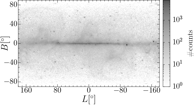
Figure 3: A gamma-ray sky map as recorded by the Large Area Telescope. The binned map of the whole sky is based on single gamma-like events with energies above 2 GeV. Point-like sources of gamma-rays and a diffuse emission from our galactic plane are clearly visible. The events can be modeled by a inhomogeneous Poisson point process.

The null hypothesis is well-defined for any choice of the bin width, because the Poisson point process does not assume an intrinsic length. However, for the application to real data, a reasonable choice of the bin width in accordance with the resolution of the detector improves the sensitivity of the analysis. A too coarse graining can hide distinct geometrical features of sources within a single pixel. If the mesh is too fine compared to the point spread function, the black and white image can easily be dominated by the random scattering of the signals.

The resolution of the LAT depends strongly on the energies of the photons. It resolves the direction of the photons within a few degrees for 1 MeV gamma-rays but with a resolution of about 0.2 degrees for energies above 2 GeV, see Acero et al., (2015). The energy of the events analyzed here ranges from 1 GeV to 1 TeV. Accordingly, we choose a bin width of about 0.2 degrees or larger.

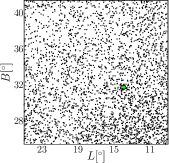
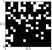
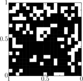
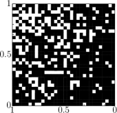
(1)                                   (2)                                       (3)

Figure 4: Excerpts from the observed gamma-ray sky map (data sets 1-3): the point patterns formed by the single events (top) and the resulting binary images for $c=2$ (bottom).

There are four contributions of the events detected by the LAT:

1. strong galactic point sources, like active galaxies of the blazar class or pulsars Acero et al., (2015),

2. diffuse radiation from galactic gas clouds, that is produced by collisions of high energetic protons and particles in the gas clouds,

3. an isotropic diffuse background from extragalactic sources, that cannot be resolved as single sources, but adds up to a homogeneous background, and

4. an isotropic background of high-energetic protons. A small fraction of the protons in the cosmic radiation are incorrectly but unavoidably classified as gamma-rays. They arrive homogeneously from all directions after a diffusion in the galactic magnetic fields.

From a statistical point of view, these four contributions can be interpreted as:

1. a strongly clustering (Matérn-type) point process,

2. an inhomogeneous Poisson point process,

3. and d) a homogeneous Poisson point process.

Here we analyze field of views that contain point sources within a homogeneous background as well as inhomogeneous diffusive radiation from the galactic disc, see Fig. 4. The first data set (upper left picture in Figure 4) contains 1041 point events. We chose as parameters $\lambda=1041$ and $m=18$, which results in $\kappa\approx 3.213$. The second data set (upper middle picture in Figure 4) contains 1339 point events ($\lambda=1339$, $m=21$ and $\kappa\approx 3.036$) and the third data set (upper right picture in Figure 4) exhibits 3193 point events ($\lambda=3193$, $m=32$ and $\kappa\approx 3.118$). For all three analysis the thresholding parameter $c$ was fixed to 2 in accordance with the insight gained in section 8. The third data set is a region in the northern Fermi bubble with diffuse radiation from gas clouds, which causes a global gradient in the point pattern, and a point source, which is marked by the diamond symbol ($\diamond$). The latter is listed in the LAT 4-year Catalog as the source J1625.1—0021 Acero et al., (2015), which is likely to be a millisecond pulsar, e.g., see Dai et al., (2016). For computing the $p$-values in Table 6 we used the asymptotic $\chi^{2}$ distribution with 1 and 3, degrees of freedom, respectively.

Table 6: Calculated $p$-values for the data sets of Figure 4

Dataset	$T_{A}$	$T_{P}$	$T_{\chi}$	$T_{c}$	$H$
1	2.560e-2	2.134e-1	4.260e-1	2.550e-2	2.616e-1
2	1.389e-3	2-927e-1	1.501e-2	2.900e-5	1.069e-1
3	2.225e-6	1.369e-3	4.507e-1	9.312e-8	2.474e-5

Table 6 shows that $T_{c}$ rejects the hypothesis of CSR for all 3 data sets, while $T_{P}$, $T_{\chi}$ and $H$ clearly fail to detect the alternative in data set 1 even for a larger level $\alpha$ like $0.1$. Data set 2 indicates the gain of power by considering the combination of 3 functionals, compared to the single functional. For data set 3 all tests, except $T_{\chi}$, detect the inhomogeneous radiation in the region of the Fermi bubble. For reference we included the $p$-values of the Hopkins and Skellam test. The quadrat count and Diggle-Cressie-Loosmore-Ford tests reject the null hypothesis, but since their power depend on parameters and on the number of Monte Carlo replications the $p$-values are omitted since the comparability is questionable.

To detect point sources, the diffuse background radiation is estimated based on maps of galactic gas clouds. These estimates are then subtracted from the data. However, because of limited observation of the gas clouds and the complex interactions between the high-energetic protons with the gas, systematic effects remain that may hide point sources in regions of strong diffuse emission.

A new approach to distinguish the signals of such hidden point sources could detect currently undetected sources in the same data. Varying the threshold, we can in principle separate the detection of point sources and diffuse emission. Moreover, our test needs no a-priori assumptions about the complex shape of the gas clouds, but nevertheless the test statistic includes geometric information of the sources in the field of view.

Here we have only applied our method as a proof of principle for a rigorous morphometric null-hypothesis test in gamma-ray astronomy. With further optimizations for applications in astroparticle physics, our approach could have the potential to detect new gamma-ray sources and help to unravel some unknown phenomena.

10 Further Comments and Conclusions

Our new tests are presented for 2-dimensional data sets due to the look-up Table 1 for Minkowski functionals. Nevertheless the table can straightforwardly be generalized to Minkowski functionals in higher dimensions in the following way. In $d$-dimensional Euclidean space ($d>2$), the $(2\times 2)$-neighborhood must be extended to a $2^{d}$-neighborhood. The total number of local configurations is therefore $2^{2^{d}}$. For each configuration, the corresponding entry in the look-up table of a Minkowski functional is given by an explicit limit of integrals. Starting with the Minkowski sum of the black pixels with a ball of radius $\varepsilon$, that is, the parallel body of the interior, an intersection with the interior of the $2^{d}$-neighborhood yields a smooth body for which the integral representation of the Minkowski functionals can be calculated, see Schröder-Turk et al., (2011). The limit $\varepsilon\rightarrow 0$ yields the entry in the look-up table. For the volume, this is equal to the number of black pixels divided by $2^{d}$, and the contribution to the surface area is given by the number of neighboring pairs of black and white pixels, divided by $2^{d-1}$. The mean width is determined by the opening angles of the edges of black pixels that are neighbors of white pixels. Similarly the local contributions to the Euler characteristic can be expressed by the corners between black and white pixels.

Furthermore, our analysis can also be applied to real data that are distorted by detector effects, like a varying camera acceptance. Instead of an initially homogeneous Poisson point process, the recorded data then follows an inhomogeneous Poisson point process with a known intensity function. Such detector effects can easily be corrected by adding Monte Carlo Poisson events or by performing a Monte Carlo post-selection Göring, (2012); Göring et al., (2013). Under the null-hypothesis for the initial data, the resulting post-processed data is again a stationary Poisson point process. If the corrections are applied locally, we can compensate even a strong suppression of signals or subtract strong known point sources Klatt, (2016).

We want to indicate some open problems related to the tests. Throughout the article, we assume that the intensity $\lambda$ of ${\cal P}_{\lambda}$ is known, so an interesting question is what effect an estimator $\widehat{\lambda}$ has in the theoretical derivations of the tests. Section 7 describes the behaviour of the Minkowski functionals under fixed alternatives, but it is still unknown the results will lead to statements regarding consistency of the tests aigainst the inhomogeneous Poisson point process and is totally open for point process alternatives with inherent dependency structure. The simulation study suggests that finding a best (data dependent) choice of the parameters $c$ and $m$ is crucial to increase the power of the tests. The presented tests contain very nice features, like very fast computation time (even for big data) and flexibility with regard to the choice of parameters, which can lead to better power performance for special alternatives.

Finally, we emphasize that the approach to analyze point patterns by means of Minkowski functionals of binary images might be the starting point of an rich and interesting path to follow for further research, and therefore give some examples.

• Simulations show that one may obtain better performing procedures by looking at more than one threshold parameter $c$. We suggest to investigate $\max_{c\in\mathbb{N}}T_{c}$ or $\sum_{c=1}^{\infty}T_{c}$ for which we expect procedures with distinctly higher power and a greater flexibility in detecting point-like or extended sources, for first simulations see Klatt, (2016).

• To detect a local deviation of CSR, we suggest to use the presented tests in a moving window approach, see Lloyd, (2007).

• In view of Hadwiger’s characterization theorem one might find a linear combination of the Minkowski functionals that is most powerful against alternatives which are additive, continuous and invariant under rigid motions.

• Tensorial Minkowski functionals are generalizations of Minkowski functionals (also called scalar Minkowski functionals), see Schneider and Weil, (2008); Schröder-Turk et al., (2011). They directly quantify the degree of anisotropy and the preferred orientation in an anisotropic system. One can easily derive a corresponding look-up table Klatt, (2016) and define analogous tests to better detect anisotropic deviations from a Poisson point process.

• The formulae given in Theorem 4.1 and 6.1 can also be used to analyze the non-occurrence of dependency in binary image (or boolean matrix) data directly by means of Minkowski functionals.

References

- Acero et al., (2015) Acero, F. et al. (2015). Fermi Large Area Telescope third source catalog. The Astrophysical Journal Supplement Series, 218(2):23.
- Atwood et al., (2009) Atwood, W. B. et al. (2009). The Large Area Telescope on the Fermi Gamma-Ray Space Telescope Mission. The Astrophysical Journal, 697(2):1071.
- Baddeley et al., (2015) Baddeley, A., Rubak, E., and Turner, R. (2015). Spatial Point Patterns: Methodology and Applications with R. Chapman and Hall/CRC Press, London.
- Baddeley and Silverman, (1984) Baddeley, A. and Silverman, B. (1984). A cautionary example on the use of second-order methods for analyzing point patterns. Biometrics, 40:1089–1094.
- Berrendero et al., (2012) Berrendero, J., Cuevas, A., and Pateiro-López, B. (2012). Testing uniformity for the case of a planar unknown support. The Canadian Journal of Statistics, 40(2):378–395.
- Berrendero et al., (2006) Berrendero, J., Cuevas, A., and Vázquez-Grande, F. (2006). Testing Multivariate Uniformity: The Distance-to-Boundary Method. The Canadian Journal of Statistics, 34(4):693–707.
- Bordoloi et al., (2017) Bordoloi, R. et al. (2017). Mapping the Nuclear Outflow of the Milky Way: Studying the Kinematics and Spatial Extent of the Northern Fermi Bubble. The Astrophysical Journal, 834(2):191.
- Byth and Ripley, (1980) Byth, K. and Ripley, B. (1980). On sampling spatial patterns by distance methods. Biometrics, 36:279–284.
- Coeurjolly, (2017) Coeurjolly, J. (2017). Median-based estimation of the intensity of a spatial point process. Annals of the Institute of Statistical Mathematics, 69:303–331.
- Core Team, (2016) Core Team, R. (2016). R: A language and environment for statistical computing. Statistical Computing.
- Cressie, (1993) Cressie, N. (1993). Statistics for Spatial Data. Wiley.
- Dai et al., (2016) Dai, X., Wang, Z., Vadakkumthani, J., and Xing, Y. (2016). Identification of candidate millisecond pulsars from fermi lat observations. Research in Astronomy and Astrophysics, 16(69):97–109.
- Dazzo et al., (2015) Dazzo, F. B., Yanni, Y. G., Jones, A., and Elsadany, A. Y. (2015). CMEIAS bioimage informatics that define the landscape ecology of immature microbial biofilms developed on plant rhizoplane surfaces. AIMS Bioengineering, 2(5):469–486.
- Ebner et al., (2016) Ebner, B., Henze, N., and Yukich, J. E. (2016). Multivariate goodness-of-fit on flat and curved spaces via nearest neighbor distances. ArXiv e-prints.
- Gaetan and Guyon, (2010) Gaetan, C. and Guyon, X. (2010). Spatial Statistics and Modeling. Springer.
- Göring, (2012) Göring, D. (2012). Gamma-Ray Astronomy Data Analysis Framework based on the Quantification of Background Morphologies using Minkowski Tensors. PhD thesis, Universität Erlangen-Nürnberg.
- Göring et al., (2013) Göring, D., Klatt, M. A., Stegmann, C., and Mecke, K. (2013). Morphometric analysis in gamma-ray astronomy using Minkowski functionals. Astronomy & Astrophysics, 555(A38).
- Gray, (1971) Gray, S. (1971). Local properties of binary images in two dimensions. IEEE Transactions on Computers, C-20(5):551–561.
- Heinrich, (2015) Heinrich, L. (2015). Gaussian limits of empirical multiparameter -functions of homogeneous Poisson processes and tests for complete spatial randomness. Lithuanian Mathematical Journal, 55(1):72–90.
- Hopkins, (1954) Hopkins, B. (1954). A new method of determining thy type of distribution of plant individuals. Annals of Botany, 18:213–227.
- Illian et al., (2008) Illian, J., Penttinen, A., Stoyan, H., and Stoyan, D. (2008). Statistical Analysis and Modelling of Spatial Point Patterns. Wiley.
- Justel et al., (1997) Justel, A., Pena, D., and Zamar, R. (1997). A multivariate Kolmogorov-Smirnov test of goodness of fit. Statistics & Probability Letters, 35:251–259.
- Karlis and Xekalaki, (2005) Karlis, D. and Xekalaki, E. (2005). Mixed Poisson Distributions. International Statistical Review, 73(1):35–58.
- Klatt, (2016) Klatt, M. (2016). Morphometry of random spatial structures in physics. PhD thesis.
- Klette and Rosenfeld, (2004) Klette, R. and Rosenfeld, A. (2004). Digital Geometry. Morgan Kaufmann, San Francisco.
- Kong and Rosenfeld, (1989) Kong, T. and Rosenfeld, A. (1989). Digital topology: Introduction and survey. Computer Vision, graphics, and Image Processing, 48:357–393.
- Kong and Rosenfeld, (1996) Kong, Y. and Rosenfeld, A., editors (1996). Topological Algorithms for Digital Image Processing. North Holland, Amsterdam.
- Lake and Keenan, (1995) Lake, D. E. and Keenan, D. M. (1995). Identifying minefields in clutter via collinearity and regularity detection. SPIE, 2496:519–530.
- Legland et al., (2007) Legland, D., Kiêu, K., and Devaux, M.-F. (2007). Computation of Minkowski Measures on 2D and 3D binary images. Image Analysis & Stereology, 26:83–92.
- Liang et al., (2001) Liang, J., Fang, K., F., H., and Li, R. (2001). Testing Multivariate Uniformity and Its Applications. Mathematics of Computation, 70(233):337–355.
- Lloyd, (2007) Lloyd, C. (2007). Local Models for Spatial Analysis. CRC Press, Boca Raton.
- Loosmore and Ford, (2006) Loosmore, N. and Ford, E. (2006). Statistical Inference using the G or K point pattern spatial statistics. Ecology, 87:1925–1931.
- Mantz et al., (2008) Mantz, H., Jacobs, K., and Mecke, K. (2008). Utilising minkowski functionals for image analysis: a marching square algorithm. Journal of Statistical Mechanics: Theory and Experiment, 2008:P12015.
- Marhuenda et al., (2005) Marhuenda, Y., Morales, D., and Pardo, M. (2005). A comparison of uniformity tests. Statistics, 39(4):315–328.
- Mecke, K. and Stoyan, D. , 2000 (Eds.) Mecke, K. and Stoyan, D. (Eds.) (2000). Statistical Physics and Spatial Statistics - The Art of Analyzing and Modeling Spatial Structures and Pattern Formation, volume 554 of Lecture Notes in Physics. Springer.
- Møller and Waagepetersen, (2003) Møller, J. and Waagepetersen, R. (2003). Statistical Inference and Simulation for Spatial Point Processes. Chapman & Hall.
- Okabe et al., (1992) Okabe, B., Boots, B., and Sugihara, K. (1992). Spatial Tesselations. Wiley.
- Penrose, (2004) Penrose, M. (2004). Random geometric graphs. Oxford University Press.
- Rinott and Rotar, (1996) Rinott, J. and Rotar, V. (1996). A Multivariate CLT for Local Dependence with Rate and Applications to Multivariate Graph Related Statistics. Journal of Multivariate Analysis, 56:333–350.
- Schneider and Weil, (2008) Schneider, R. and Weil, W. (2008). Stochastic and Integral Geometry. Springer.
- Schröder-Turk et al., (2011) Schröder-Turk, G. E. et al. (2011). Minkowski tensor shape analysis of cellular, granular and porous structures. Advanced Materials, 23:2535–2553.
- Shaked, (1980) Shaked, M. (1980). On mixtures from exponential families. Journal of the Royal Statistical Society Series B, 42:192–198.
- Skellam, (1954) Skellam, J. (1954). Appendix to article by Hopkins (1954). Annals of Botany, 18:226–227.
- Tenreiro, (2007) Tenreiro, C. (2007). On the Finite Sample Behavior of Fixed Bandwidth Bickel-Rosenblatt Test for Univariate and Multivariate Uniformity. Communications in Statistics - Simulation and Computation, 36:827–846.
- Viktorova and Chistyakov, (1966) Viktorova, I. I. and Chistyakov, V. P. (1966). Some generalizations of the test of empty boxes. Theory of Probability and its applications, 11(2):270–276.
- Wheeler, (2007) Wheeler, D. C. (2007). A comparison of spatial clustering and cluster detection techniques for childhood leukemia incidence in ohio, 1996-2003. International Journal of Health Geographics, 6(13).