Generalized symmetry relations for connection matrices in the phase-integral method

Abstract

We consider the phase-integral method applied to an arbitrary ordinary linear differential equation of the second-order and study how its symmetries affect the connection matrices associated with its general solution. We reduce the obtained exact general relation for the matrices to its limiting case introducing a concept of the effective Stokes constant. We also propose a concept of an effective Stokes diagram which can be a useful tool for analyzing difficult equations. We show that effective Stokes domains which can be overlapped by a symmetry transformation are associated with the same effective Stokes constant and can be described by the same analytical function. Basing on the derived symmetry relations, we propose a way to write functional equations for the effective Stokes constants. Finally, we provide a generalization of the derived symmetry relations for an arbitrary order linear system of the ordinary linear differential equations. This work also contains an example of usage of the presented ideas in a case of a real physical problem. To access the HTML version of the paper & discuss it with the author, visit https://enabla.com/pub/1108.

1 Introduction

Consider an arbitrary ordinary linear second-order differential equation written in the form of a stationary one-dimensional Schrödinger equation

$$\widehat{L}(z,\bm{\lambda})y(z,\bm{\lambda})=0,\quad\widehat{L}(z,\bm{\lambda})=\frac{\mathrm{d}^{2}}{\mathrm{d}z^{2}}+R(z,\bm{\lambda}),$$ (1)

where $\bm{\lambda}$ is a set of the problem’s parameters. Its approximate local solution can be obtained with use of the phase-integral approximation generated from the unspecified base function [1]:

$$y(z) \sim c_{+}y_{+}(z)+c_{-}y_{-}(z),$$ (2a)

$$y_{\pm}(z) =q(z,\bm{\lambda})^{-1/2}\exp[\pm\mathrm{i}\omega(z)],$$ (2b)

$$\omega(z) =\int_{(z_{0})}^{z}q(\xi,\bm{\lambda})\mathrm{d}\xi,$$ (2c)

where the explicit form of $q(z)$ depends on the order and particular type of the approximation. The simplest and the best-known type is one of the WKBJ [2, 3, 4, 5]; it takes the form (2) with $q(z,\bm{\lambda})=\sqrt{R(z,\bm{\lambda})}$.

The function $\omega(z)$ is the phase integral, and therefore we call $q(\xi,\bm{\lambda})$ the phase integrand. Also, we will refer to $z_{0}$ as a basepoint. A meaning of the brackets in the lower limit of integration is a bit tricky; such a notation was introduced by Fröman and Fröman [6] to make the integral look similar for all orders of approximation. In the lowest order and, particularly, in case of the WKBJ approximation, this integral is just a usual integral from $z_{0}$ to $z$.

The general solution (2a) is a local, not global, solution of (1), i.e. the coefficients $c_{\pm}$ vary from one point of the complex plane to another. Provided that

$$\varepsilon=q^{-3/2}\mathrm{d}^{2}q^{-1/2}/\mathrm{d}z^{2}+(R-q^{2})/q\ll 1$$ (3)

in the considered area of the complex plane, the variations are, in general, slow but may have abrupt changes on the so-called Stokes lines (Stokes phenomenon [7, 8, 9, 1]). Such changes have a form of a single-parameter linear transform [9]; the parameter is called the Stokes constant. Knowing all Stokes constants associated with a particular equation makes it possible to obtain a globally defined approximate solution of (1), and the phase-integral method provides a simple way to do it [9, 8]. Unfortunately, there are very few cases when this method allows finding all the constants exactly, so approximations of different kinds are commonly used [8, 25]. This happens mostly because of a lack of the exact equations for the Stokes constants.

The phase-integral approximation has an extensive application in various fields of physics. It is widely used in quantum mechanics and nuclear physics to calculate energy spectrum and study wave functions for both Schrödinger [10, 11, 12] and Dirac [13] equations. It is successfully used in plasma physics to study electromagnetic waves’ scattering characteristics [14, 15] as long as many problems in this area can be reduced to a problem of linear coupling [16, 17, 18]. It is also useful in other branches of physics such as high-energy physics [19] or general relativity [20, 21, 22]. Among the publications devoted to the phase-integral method there are both classical monographs [23, 24, 8, 9, 1] and modern attempts to improve its accuracy [25, 26]. In the present paper we provide a way to reduce the number of independent Stokes constants with use of the symmetries of (1).

The paper is organized as follows. In Section 2 we recall briefly the F-matrix formalism and introduce a concept of the effective Stokes constant. We also give a matrix formulation of the well-known Heading’s rules for analytical continuation; such formulation appears to be much more convenient for our purposes than the traditional one, which can be found, for example, in [8]. In Section 3 we derive the symmetry relations for the connection matrices in the most common case of the second-order differential equation. In Section 4 we simplify the relations by reducing F-matrix to its limiting form and obtain the symmetry relations for the effective Stokes constants. In this section we also discuss a possibility of writing functional equations for effective Stokes constants. In Section 5 a concept of an effective Stokes diagram is presented; this concept is a natural consequence of the effective Stokes constants’ usage. In Section 6 we present an example of a real physical problem solved with the help of our technique; the symmetry relations for effective Stokes constants are used to find the exact form of reflection and transmission coefficients for the Weber equation. In Section 7 we discuss an applicability of the symmetry relations derived in Section 3 for the case of an arbitrary order system of ordinary linear differential equations. And, finally, in Section 8 are the conclusions.

2 Connection matrices and effective Stokes constants

As it was mentioned in the previous section, the coefficients $c_{\pm}$ vary from one point of the complex plane to another. Taking into consideration the linearity of (1), these variations can by described formally by means of the F-matrices [1]:

$$\bm{\psi}(z_{2})=\bm{F}(z_{2},z_{1})\bm{\psi}(z_{1}),$$ (4)

where $\bm{\psi}(z)=[{c_{+}(z),c_{-}(z)}]^{\mathrm{T}}$ and ‘T’ denotes the transpose operation. In principle, F-matrix can be obtained exactly from the corresponding differential equation [1]; then, the approximate solution (2a) with $c_{\pm}=c_{\pm}(z)$ becomes exact.

F-matrix does not depend on the $\bm{\psi}-$vectors, i.e. on the initial/boundary conditions of (1), and represents properties of its general solution. As long as the general solution may have branch points, F-matrix can depend on the particular path $\gamma$ of analytical continuation; we will indicate the path by writing $\bm{F}[\gamma]$ instead of $\bm{F}(z_{2},z_{1})$, if necessary.

F-matrix also depends on the chosen system of approximate solutions $y_{\pm}$ and, particularly, on the chosen basepoint $z_{0}$. Consider equation (1) and some definite type of the phase-integral approximation with $q(z,\bm{\lambda})$ as a phase integrand and $z_{0}$ as a basepoint. Then, consider two points $z_{1,2}(\bm{\lambda})$ of the complex plane and an oriented curve $\gamma$ connecting these points; according to the definition (4) of the F-matrix, $\bm{F}[\gamma]$ relates coefficients $c_{\pm}$ at the ends of the curve. We say that $\bm{F}_{q,z_{0}}[\gamma]$ performs an analytical continuation of the general solution of (1) along the oriented curve $\gamma$ in the system $\{q,z_{0}\}$; we will indicate the system by the corresponding subscript of the F-matrix, if necessary.

Consider equation (1) and two F-matrices, $\bm{F}_{q,z_{0}}[\gamma]$ and $\bm{F}_{q,\tilde{z}_{0}}[\gamma]$, performing an analytical continuation of the general solution along the oriented curve $\gamma$; the matrices represent the same analytical continuation, but written with use of different basepoints. They can be related as

$$\bm{F}_{q,\tilde{z}_{0}}[\gamma]=\bm{W}[\tilde{z}_{0},z_{0}]\bm{F}_{q,z_{0}}[\gamma]\bm{W}[z_{0},\tilde{z}_{0}],$$ (5)

where

$$\bm{W}[b,a]=\left(\begin{array}[]{*{2}{c}}\mathrm{e}^{\mathrm{i}\int_{(a)}^{(b)}q(z,\bm{\lambda})\mathrm{d}z}&0\\ 0&\mathrm{e}^{-\mathrm{i}\int_{(a)}^{(b)}q(z,\bm{\lambda})\mathrm{d}z}\end{array}\right);$$ (6)

this follows directly from (4) and (2).

Then, consider the same differential equation, but different F-matrices $\bm{F}_{q,z_{0}}[\gamma]$ and $\bm{F}_{-q,z_{0}}[\gamma]$; this is the simplest nontrivial example of F-matrices representing the same analytical continuation, but written with use of different phase integrands. Accurate to insignificant constant multiplier connected with slow $q(z,\bm{\lambda})^{-1/2}$ dependency, these two systems of base phase-integral approximate solutions differ by their order; the difference can be naturally described by a permutation matrix $\bm{P}_{\sigma}$:

$$\bm{F}_{-q,z_{0}}[\gamma]=\bm{P}_{\sigma}\bm{F}_{q,z_{0}}[\gamma]\bm{P}_{\sigma}^{-1},\quad\bm{P}_{\sigma}=\left(\begin{array}[]{*{2}{c}}0&1\\ 1&0\end{array}\right).$$ (7)

The permutation matrix in this relation maps the system $\{q,z_{0}\}$ to the system $\{-q,z_{0}\}$, but the direction of the mapping is insignificant in case of $2\times 2$ matrices because then $\bm{P}_{\sigma}^{-1}=\bm{P}_{\sigma}$.

In the limit (3) of small epsilon, F-matrix represents the linear transformation mentioned in Section 1 and can be approximately expressed in terms of the corresponding Stokes constants and phase integrals. As long as the limiting form of F-matrix is more common and more convenient from the practical point of view, we will end the present section with its detailed description.

Let’s start with some basic definitions. Hereinafter we will refer to a point $z$ of the complex plane as a singular point if epsilon from (3) is infinitely large in such a point; its vicinity will be referred to as an interaction area. At every point $z$ of the complex plane except the singularities we will distinguish two orthogonal directions. Let’s define the Stokes direction as a direction with $\mathrm{Re}\left[q(z,\bm{\lambda})\mathrm{d}z\right]=0$ and the anti-Stokes direction as a direction with $\mathrm{Im}\left[q(z,\bm{\lambda})\mathrm{d}z\right]=0$. We will also use a notion of the Stokes (anti-Stokes) field as a set of Stokes (anti-Stokes) directions for the entire complex plane. Following [9, 8], we introduce Stokes (anti-Stokes) lines as a paths along Stokes (anti-Stokes) field emanating from the singularities. Any domain of the complex plane bounded by the Stokes (anti-Stokes) lines and containing no other Stokes (anti-Stokes) lines will be referred to as the anti-Stokes (Stokes) domain. Particularly, if $q^{2}(z,\bm{\lambda})\sim z^{n}$ as $z$ goes to complex infinity, then there are $n+2$ Stokes (anti-Stokes) domains in the vicinity of the infinity – we will call such domains the Stokes (anti-Stokes) wedges. Asymptotic phase-integral solutions (2b) oscillate along anti-Stokes lines with constant flow and increase (or decrease) exponentially with constant phase along Stokes lines. The increasing (decreasing) solution will be called dominant (subdominant) in a given Stokes domain. Also, the complex plane with singular points, Stokes and anti-Stokes lines and branch cuts associated with a branching structure of asymptotic solutions (2) will be referred to as a Stokes diagram.

Consider a Stokes domain and the F-matrix associated with crossing this domain in counterclockwise direction relatively to the chosen basepoint. According to estimates made by Fröman and Fröman [1], in a limit (3) of small epsilon such F-matrix can be approximately written as either $\bm{S}[s]$ or $\bm{S}^{\mathrm{T}}[s]$, where

$$\bm{S}[s]=\left(\begin{array}[]{*{2}{c}}1&0\\ s&1\end{array}\right)$$ (8)

and $s$ is a Stokes constant associated with the domain. In the present paper, we will call such a constant an effective Stokes constant to emphasize its difference from the traditional one. Indeed, there can be multiple Stokes lines in the Stokes domain, and every such line is associated with its own traditional Stokes constant [9, 8], whereas the effective Stokes constant is associated with the whole Stokes domain. It is also worth mentioning that every effective Stokes constant can be expressed in terms of the traditional ones; it becomes clear from the reasoning presented in Appendix A.

We will refer to $\bm{S}$ as a Stokes operator. As it can be inferred from the Frömans estimates, we must use $\bm{S}$ for a Stokes domain where $y_{+}$ is dominant and $\bm{S}^{\mathrm{T}}$ otherwise. The rules for the Stokes operator are analogous to the traditional Heading’s rules for analytical continuation, presented, for example, in [9, 8]. As it follows from the previous discussion and from the Heading’s rules itself, both traditional and effective Stokes constants depend on basepoint. In [9, 8] the change of the basepoint is called ‘reconnection’, thus we will refer to $W[b,a]$ introduced by Equation 6 as a reconnection operator.

Aside from crossing Stokes line and changing basepoint, the Heading’s rules include the rule for crossing a branch cut associated with the branching structure of the phase-integral approximate solutions (2b). According to Fröman and Fröman [1], the operator, describing crossing a branch cut emerging from the first order zero of the squared phase integrand $q^{2}(z,\bm{\lambda})$ in counterclockwise direction, takes the form

$$\bm{C}=\left(\begin{array}[]{*{2}{c}}0&-\mathrm{i}\\ -\mathrm{i}&0\end{array}\right).$$ (9)

In case of the different order of the branch point the operator must be raised to an appropriate power.

With help of these three operators, $\bm{S}$, $\bm{W}$ and $\bm{C}$, the reader can perform any analytical continuation far away from any singularities; the matrix formulation of the traditional Heading’s rules appears to be much more convenient for our purposes.

3 Symmetry relations for the connection matrices

Let’s clarify what we mean by a symmetry of a given equation. Here we introduce three operators $\hat{f}(z,\bm{\lambda})$, $\hat{g}(z,\bm{\lambda})$ and $\hat{h}(z,\bm{\lambda})$ such that

$$\hat{f}:\{y\}\rightarrow\{y\},\quad\hat{g}:\{z\}\rightarrow\{z\},\quad\hat{h}:\{\bm{\lambda}\}\rightarrow\{\bm{\lambda}\},$$ (10)

i.e. $\hat{f}$ (complex conjugation, multiplication, etc.) acts on the set of functions, preserving the structure of their Stokes diagrams, $\hat{g}$ (complex conjugation, invertible function of complex variable, etc.) acts on the field of complex numbers, and $\hat{h}$ (complex conjugation, analytical function of $\bm{\lambda}$, etc.) acts on the parameter’s space. As it will be seen from the following discussion, the restriction on $\hat{g}$ to be invertible is crucial.

We define any set of operators $\{\hat{f}(z,\bm{\lambda}),\hat{g}(z,\bm{\lambda}),\hat{h}(z,\bm{\lambda})\}$ as a symmetry transformation of (1) if for any its solution $y(z,\bm{\lambda})$ there is another solution $\tilde{y}(z,\bm{\lambda})$ such that $\tilde{y}(z,\bm{\lambda})=\hat{f}(z,\bm{\lambda})y(\hat{g}(z,\bm{\lambda})z,\hat{h}(z,\bm{\lambda})\bm{\lambda})$, i.e.

$$\widehat{L}(z,\bm{\lambda})y(z,\bm{\lambda})\equiv 0\ \Longrightarrow\ \widehat{L}(z,\bm{\lambda})\left[\hat{f}(z,\bm{\lambda})y(\hat{g}(z,\bm{\lambda})z,\hat{h}(z,\bm{\lambda})\bm{\lambda})\right]\equiv 0.$$ (11)

As it follows from the definition, $\tilde{y}(z,\bm{\lambda})$ as well as $y(z,\bm{\lambda})$ can be written in the form (2a), but with different coefficients $c_{\pm}$ and $\tilde{c}_{\pm}$ correspondingly. This difference and, as a consequence, restrictions on the connection matrices can be obtained directly by applying the symmetry transformation to (2b) as it was done in [27] for the special case analysed by Frömans, but we prefer more intuitive derivation.

Let’s choose some definite type of the phase-integral approximation with $q(z,\bm{\lambda})$ as the phase integrand; this phase integrand will be used all throughout the present section. Consider $y(z,\bm{\lambda})$, some solution of (1), and its analytical continuation along the oriented curve $\gamma$, performed in the system $\{q,z_{0}\}$:

$$y(z,\bm{\lambda}):\ \gamma\ \longrightarrow\ \bm{F}_{q,z_{0}}[\gamma,\bm{\lambda}].$$ (12)

Then, consider another solution of (1), $\tilde{y}(z,\bm{\lambda})$, and its analytical continuation along the same curve, but performed with use of different basepoint:

$$\tilde{y}(z,\bm{\lambda}):\ \gamma\ \longrightarrow\ \bm{F}_{q,\tilde{z}_{0}}[\gamma,\bm{\lambda}].$$ (13)

As it follows from the previous discussion, $\bm{F}_{q,z_{0}}[\gamma,\bm{\lambda}]$ and $\bm{F}_{q,\tilde{z}_{0}}[\gamma,\bm{\lambda}]$ represent the same operation in different bases and can be related with use of a reconnection operator. On the other hand, and this is much more important, if the solution $\tilde{y}(z,\bm{\lambda})$ is connected with $y(z,\bm{\lambda})$ through the symmetry transformation $\{\hat{f}(z,\bm{\lambda}),\hat{g}(z,\bm{\lambda}),\hat{h}(z,\bm{\lambda})\}$, its analytical continuation along the curve $\gamma$ can be obtained directly from the corresponding continuation of $y(z,\bm{\lambda})$ by a formal application of the symmetry transformation:

$$\tilde{y}(z,\bm{\lambda})\equiv\hat{f}y(\hat{g}z,\hat{h}\bm{\lambda}):\ \gamma\ \longrightarrow\ \hat{f}\bm{F}_{q,z_{0}}[\hat{g}\gamma,\hat{h}\bm{\lambda}].$$ (14)

We underline that this last analytical continuation is performed along the same curve $\gamma$ as it was in the previous cases because any curve is the ordered set of allowed values of $z$, not $\hat{g}z$. Thus, $\hat{f}\bm{F}_{q,z_{0}}[\hat{g}\gamma,\hat{h}\bm{\lambda}]$ and $\bm{F}_{q,\tilde{z}_{0}}[\gamma,\bm{\lambda}]$ represent the same analytical continuation, but performed with use of different systems of base approximate phase-integral solutions (2b). It is crucial that the systems can differ not only by the basepoints’ location, but also by the functions $y_{\pm}$. Indeed, accurate to insignificant constant multiplier connected with slow $q(z,\bm{\lambda})^{-1/2}$ dependency, there are two possible mappings implemented by the symmetry transformation: $y_{\pm}\rightarrow y_{\pm}$, or $y_{\pm}\rightarrow y_{\mp}$; such mappings were considered in the previous section and can be described by a permutation matrix $\bm{P}_{\sigma}$.

Now, we are ready to write the final relation for the F-matrices. A formula expressing this relation is shown below:

$$\bm{P}_{\sigma}^{-1}\left\{\hat{f}\bm{F}_{q,z_{0}}\left[\hat{g}\gamma,\hat{h}\bm{\lambda}\right]\right\}\bm{P}_{\sigma}$$ (15)

$$\qquad=\bm{W}\left[\hat{g}^{-1}z_{0}(\hat{h}\bm{\lambda}),\tilde{z}_{0}(\bm{\lambda})\right]\bm{F}_{q,\tilde{z}_{0}}\left[\gamma,\bm{\lambda}\right]\bm{W}\left[\tilde{z}_{0}(\bm{\lambda}),\hat{g}^{-1}z_{0}(\hat{h}\bm{\lambda})\right].$$

The inverse operator $\hat{g}^{-1}$ in the formula appears due to the variableexchange in the phase integral:

$$\hat{g}\int_{(z_{0})}^{z}q(\xi)\mathrm{d}\xi=\int_{(z_{0})}^{\hat{g}z}q(\xi)\mathrm{d}\xi=\int_{(\hat{g}^{-1}z_{0})}^{z}q(\hat{g}\xi)\mathrm{d}\hat{g}\xi.$$ (16)

An explicit form of the permutation matrix $\bm{P}_{\sigma}$ can be determined by a direct application of the symmetry transformation to the base functions $y_{\pm}$.

The relation (15) has a fairly transparent structure. Indeed, assume we chose $y_{\pm}$ as a base system of phase-integral approximate solutions with $\hat{g}^{-1}z_{0}(\hat{h}\bm{\lambda})$ as a basepoint. To implement the analytical continuation in such a base with use of known F-matrices $\hat{f}\bm{F}_{q,z_{0}}[\hat{g}\gamma,\hat{h}\bm{\lambda}]$ and $\bm{F}_{q,\tilde{z}_{0}}[\gamma,\bm{\lambda}]$, we have to either change the basepoint from $\hat{g}^{-1}z_{0}(\hat{h}\bm{\lambda})$ to $\tilde{z}_{0}$ and apply $\bm{F}_{q,\tilde{z}_{0}}[\gamma,\bm{\lambda}]$ (right hand side of (15)) or choose an appropriate order of the base functions $y_{\pm}$ and apply $\hat{f}\bm{F}_{q,z_{0}}[\hat{g}\gamma,\hat{h}\bm{\lambda}]$ (left hand side of (15)); our relation reflects the equivalence of these two approaches.

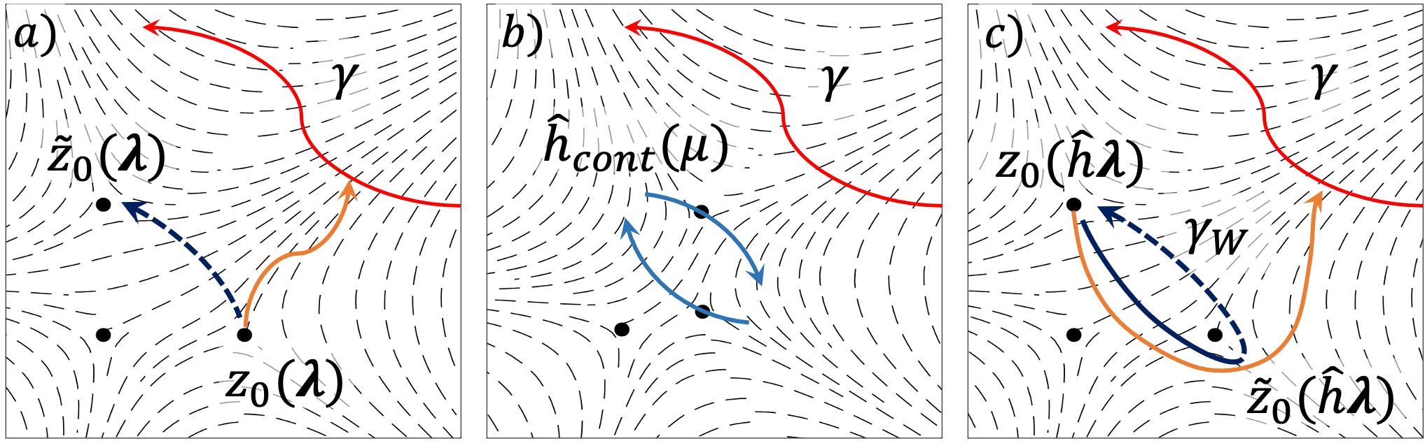
Figure 1: Stokes field for $q(z)=\sqrt{z(z-1)(z-\mathrm{i})}$ and its metamorphosis under the action of $\hat{h}$ swapping singular points in $z=1$ and $z=\mathrm{i}$ as shown in the panel (b) (${\hat{f}=\hat{g}=1}$). This is an example of how to determine $\gamma_{W}$, the integration path for the reconnection operator $\bm{W}\left[\hat{g}^{-1}z_{0}(\hat{h}\bm{\lambda}),\tilde{z}_{0}(\bm{\lambda})\right]$ from (15). In the panel (a) the curve $\gamma$ (continuous red) and two different basepoints are shown, $z_{0}(\bm{\lambda})$ and $\tilde{z}_{0}(\bm{\lambda})$; the continuous orange line illustrates the path used for the definition of the phase integral $\omega(z)$ from (2), and the dashed dark blue line shows a path we want to use for the reconnection from $z_{0}$ to $\tilde{z}_{0}$. In the panel (b), some intermediate state of the continuously parameterized symmetry transformation $\hat{h}_{cont}(\mu)$ is shown. Finally, in the right panel (c) the result of the transformation and the path $\gamma_{W}$ are shown; the first part of the path $\gamma_{W}$ (solid dark blue line) corresponds to the symmetry transformation itself, and the second part (dashed dark blue line) corresponds to the reconnection path shown in the panel (a).

A presence of the reconnection operator $\bm{W}\left[\hat{g}^{-1}z_{0}(\hat{h}\bm{\lambda}),\tilde{z}_{0}(\bm{\lambda})\right]$ in (15) implies an integration along some path $\gamma_{W}$ in the complex plane; thus, the resulting relation may depend on this path if the phase integrand has poles or branch points. This fact forces us to consider not only the final result of the symmetry transformation, but even how exactly it was performed; i.e., we have to parameterize $\hat{g}$ and $\hat{h}$ operators. This can be done by introducing of an auxiliary variable $\mu$ varying from $0$ to $1$ such that, for example, $\hat{g}_{cont}(\mu)=1+\mu(\hat{g}-1)$, and $\hat{g}_{cont}(1)=\hat{g}$. Then, the path $\gamma_{W}$ can be determined in the following way: one have to fix the integration path used in the phase-integral $\omega(z)$ from (2) for the basepoint $z_{0}(\bm{\lambda})$ (continuous orange line in Fig. 1(a)), study how this path deforms under our transformation, go along this deformed path from $\hat{g}^{-1}z_{0}(\hat{h}\bm{\lambda})$ to $z_{0}(\bm{\lambda})$, and then perform just a usual reconnection from $z_{0}(\bm{\lambda})$ to $\tilde{z}_{0}(\bm{\lambda})$ as if there was no symmetry transformation involved. Note that $\hat{g}^{-1}z_{0}(\hat{h}\bm{\lambda})=\tilde{z}_{0}(\bm{\lambda})$ doesn’t in general mean that the reconnection operator is the identity operator; in principle, $\gamma_{W}$ can form closed loops like the one in Fig. 1.

The relation (15) is actually a generalization of the symmetry relations obtained by Fröman and Fröman [27]. It takes the form presented in their article with $\{\hat{f}=\hat{g}=\hat{h}=c.c.\}$, where $c.c.$ stands for the complex conjugation, for the first case they considered, and with $\{\hat{g}=-1;\hat{f}=\hat{h}=1\}$ for the second case.

4 Symmetry relations and functional equations
for effective Stokes constants

The symmetry relation (15) is exact and quite general, but it is not very useful from the practical point of view because F-matrices are usually used in a limit (3) of small epsilon; thus, analogous symmetry relations for the Stokes constants appear to be more convenient. In the present section, we obtain the symmetry relations for the effective Stokes constants and discuss the consequences of the relations.

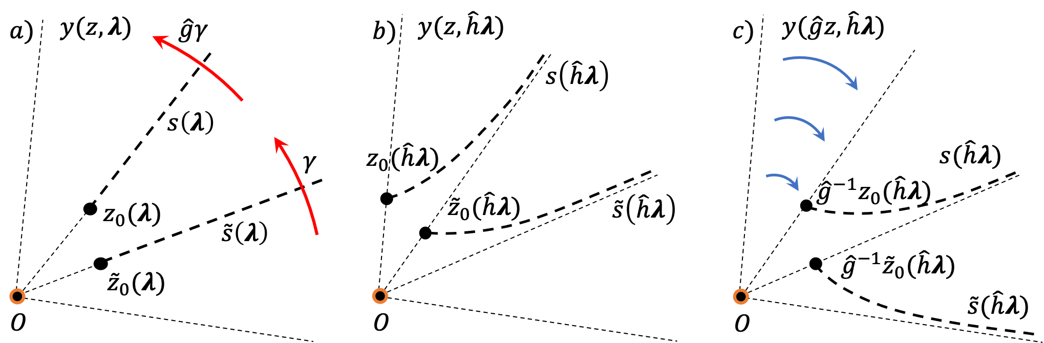
Figure 2: An illustration for Eq. 17 with $\hat{f}=1$; the point $O$ is a center of the rotation $\hat{g}$, the thin straight dashed lines emanating from $O$ represent the Stokes directions, the bold dashed lines emanating from the base points stand for the Stokes lines, and $\hat{g}^{-1}z_{0}(\hat{h}\bm{\lambda})=z_{0}(\bm{\lambda})$. Here you can see how the Stokes constants $s$ and $\tilde{s}$ from different Stokes directions can be related due to the overlap generated by the symmetry transformation: in the left panel (a) the two paths $\gamma$ and $\hat{g}\gamma$ are shown; in the middle panel (b) only the parameter transformation $\hat{h}$ is applied moving the basepoints $z_{0}$ and $\tilde{z}_{0}$, and in the right panel (c) the rotation $\hat{g}$ finishes the transformation overlapping the Stokes direction corresponding to $s(\hat{h}\bm{\lambda})$ with the one which previously corresponded to $\tilde{s}(\bm{\lambda})$.

Consider an oriented curve $\gamma$ located far away from any interaction area and crossing one Stokes domain associated with the effective Stokes constant $\tilde{s}$ in counterclockwise direction relative to the chosen basepoint as shown in Fig. 2. Consider another Stokes domain associated with another effective Stokes constant $s$ such that the transformed oriented curve $\hat{g}\gamma$ also crosses this second domain far from any singularity. Using the relation (15) for the F-matrices, its limiting form described in the Section 2, and the rules for the Stokes operators, we obtain

$$\bm{S}^{(\mathrm{T})}\left[\hat{f}s(\hat{h}\bm{\lambda})\right] =\bm{W}\left[\hat{g}^{-1}z_{0}(\hat{h}\bm{\lambda}),\tilde{z}_{0}(\bm{\lambda})\right]$$ (17)

$$\quad\times\bm{S}^{(\mathrm{T})}\left[\tilde{s}(\bm{\lambda})\right]\bm{W}\left[\tilde{z}_{0}(\bm{\lambda}),\hat{g}^{-1}z_{0}(\hat{h}\bm{\lambda})\right],$$

where $s$ and $\tilde{s}$ are the effective Stokes constants having $z_{0}$ and $\tilde{z}_{0}$ as their basepoints, and $\bm{S}^{(\mathrm{T})}$ can be either $\bm{S}$ or $\bm{S}^{\mathrm{T}}$. The choice in the right hand side of (17) must be made on the basis of general rules from Section 2: we use $\bm{S}$ for the Stokes domain associated with $\tilde{s}(\bm{\lambda})$ if $y_{+}$ is dominant and $\bm{S}^{\mathrm{T}}$ otherwise. In the left hand side of (17) we have to use the same form as in the right hand side; the rule is a consequence of the permutation matrix presence in (15).

The relation obtained above allows us to take a fresh look at the nature of the different effective Stokes constants. Two different Stokes domains which can be overlapped by the transformation $\hat{g}$ are actually associated with the same effective Stokes constant but evaluated in the different points of the parameters’ space. In particular, every set of Stokes wedges can be described by a single multidimensional analytical complex function $s(\bm{\lambda})$.

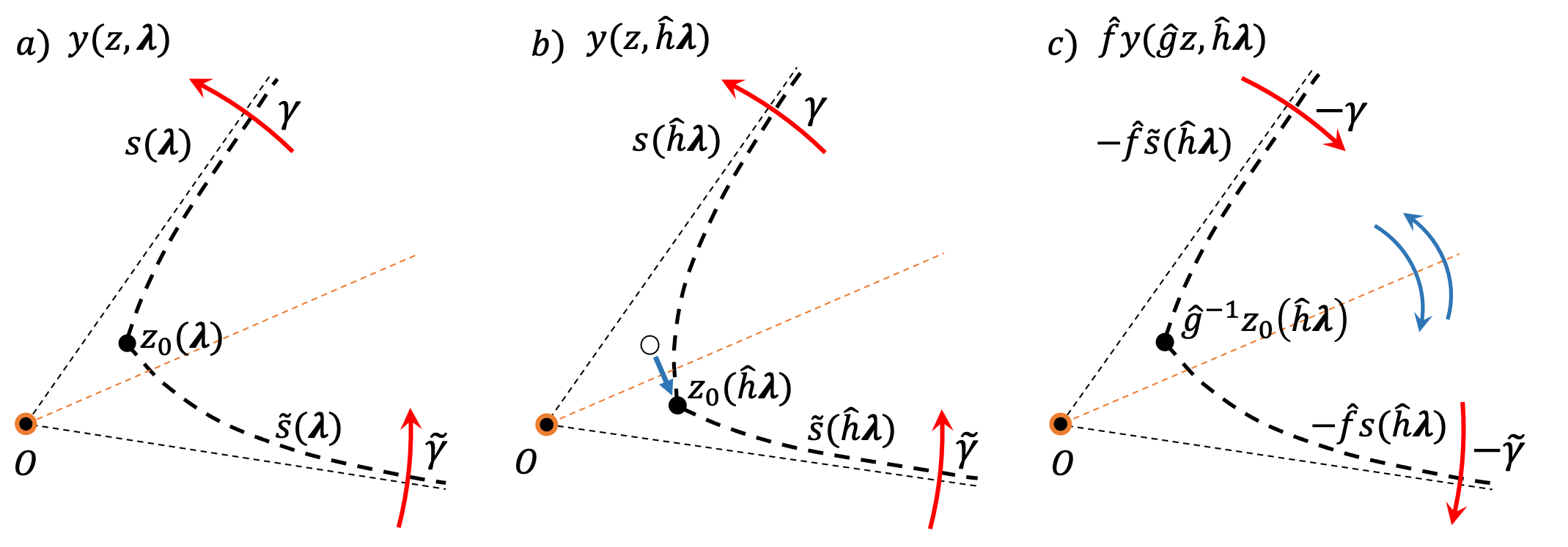
Figure 3: An illustration for the “conjugation” symmetry for which the complex conjugation symmetry discussed around the Eq. 18 stands as a special case. The orange dashed line starting at the point $O$ represents the conjugation axis, the thin straight dashed lines emanating from $O$ represent the Stokes directions, and the bold dashed lines emanating from the basepoint $z_{0}$ stand for the Stokes lines; for the simplicity we assume here that $z_{0}\equiv\tilde{z}_{0}$. You can see how the Stokes constant $s$ can be related to its “mirror image” $\tilde{s}$ with minus sign: the “conjugation” applied between the steps (b) and (c) not only overlapped different Stokes directions but also inverted the directions on the oriented curves $\gamma$ and $\tilde{\gamma}$.

Consider an important special case of a complex conjugation symmetry, analysed by Frömans [27]. For every equation which is real on the real axis the symmetry $\hat{f}=\hat{g}=\hat{h}=c.c.$ holds, i.e. $\widehat{L}^{*}(z^{*},\bm{\lambda}^{*})=\widehat{L}(z,\bm{\lambda})$ and

$$\bm{S}^{(\mathrm{T})}\left[-s^{*}(\bm{\lambda}^{*})\right]=\bm{W}\left[z_{0}^{*}(\bm{\lambda}^{*}),\tilde{z}_{0}(\bm{\lambda})\right]\bm{S}^{(\mathrm{T})}\left[\tilde{s}(\bm{\lambda})\right]\bm{W}\left[\tilde{z}_{0}(\bm{\lambda}),z_{0}^{*}(\bm{\lambda}^{*})\right].$$ (18)

A minus sign before the effective Stokes constant in the left hand side of (18) is a result of the complex conjugation symmetry; it appears for any transformation $\hat{g}$ which changes the direction of analytical continuation relative to the chosen basepoint since the Stokes constant is defined for the counterclockwise direction, see Fig. 3. If $\tilde{z}_{0}(\bm{\lambda})=z_{0}^{*}(\bm{\lambda}^{*})$ and $\bm{\lambda}$ is real, we obtain a result $s^{*}(\bm{\lambda})=-\tilde{s}(\bm{\lambda})$, which can be inferred from the symmetry relations presented in [27]. If furthermore $s=\tilde{s}$, we get an important and extremely simple relation $s^{*}(\bm{\lambda})=-s(\bm{\lambda})$, i.e. such effective Stokes constant is purely imaginary provided $\bm{\lambda}$ is real.

Another important case of (17) is a case with $\hat{g}=1$ and $z_{0}(\bm{\lambda})=\tilde{z}_{0}(\bm{\lambda})$:

$$\bm{S}^{(\mathrm{T})}\left[\hat{f}s(\hat{h}\bm{\lambda})\right]=\bm{W}\left[z_{0}(\hat{h}\bm{\lambda}),z_{0}(\bm{\lambda})\right]\bm{S}^{(\mathrm{T})}\left[s(\bm{\lambda})\right]\bm{W}\left[z_{0}(\bm{\lambda}),z_{0}(\hat{h}\bm{\lambda})\right].$$ (19)

Such case is relevant for every equation. The obtained relation is a functional equation for the considered effective Stokes constant. Usually such equation helps to illuminate a branching structure of the effective Stokes constant and write it as a new single-valued function multiplied by the known multivalued one. It is worth mentioning that even simple formal symmetries like $\{\hat{h}=\mathrm{e}^{2\mathrm{i}\pi},\hat{g}=\hat{f}=1\}$ may produce nontrivial functional equations; it happens every time when the reconnection operator differs from unity.

5 Effective Stokes diagram

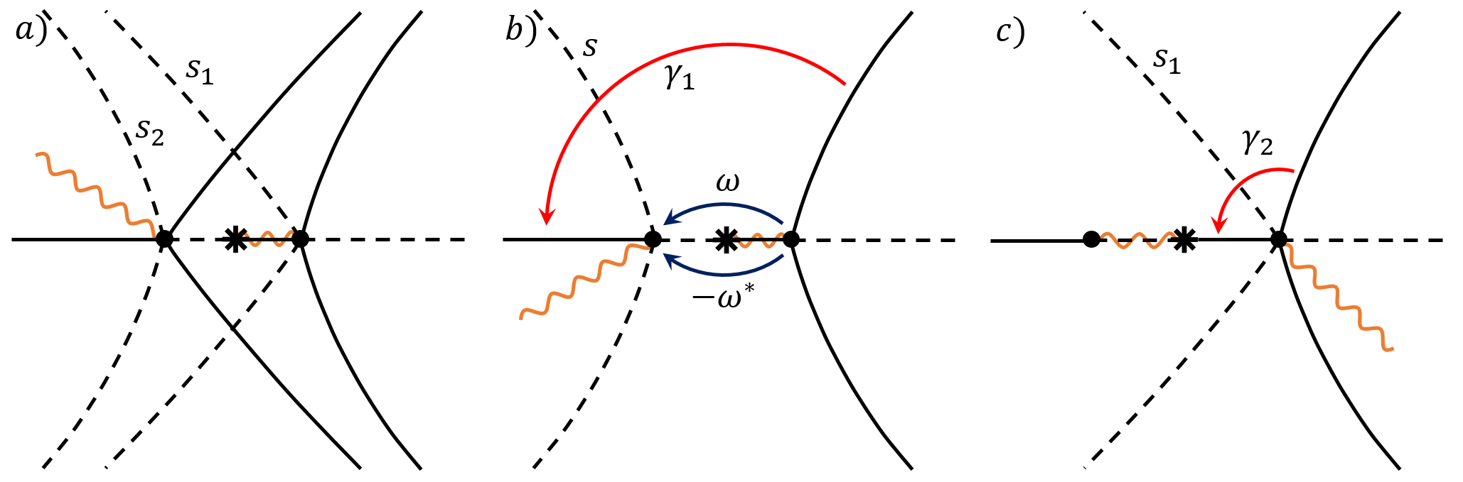
Figure 4: Stokes diagrams for $q(z,g)=\sqrt{-z+g^{2}/z}$; Stokes lines are dashed. (a) A traditional Stokes diagram; dots and stars indicate correspondingly zeros and poles of the phase integrand. (b) An effective Stokes diagram with a specified path of analytical continuation $\gamma_{1}$. (c) An effective Stokes diagram with a different path of analytical continuation $\gamma_{2}$. The Stokes constant $s_{1}$ is meaningful only if $g\gg 1$ and all the singularities are far away from each other – otherwise the phase-integral approximation itself fails between the pole and the right zero and the exact F-matrix must be used.

The concept of the effective Stokes constant allows us to introduce a notion of the effective Stokes line. Since every Stokes domain can be described by a single effective Stokes constant, we can visualize this fact by plotting a single effective Stokes line instead of a set of traditional Stokes lines. Similarly, every set of anti-Stokes lines located in the same anti-Stokes domain can be replaced by a single effective anti-Stokes line; such a line now is just a borderline separating different Stokes domains. A Stokes diagram consisting of effective Stokes and anti-Stokes lines will be referred to as an effective Stokes diagram. As it can be seen from Figures 4 and 5, effective diagram is not unique. It can be plotted differently depending on a chosen path of analytical continuation (Figure 4); that is why it is usually convenient to specify the path right on the diagram. But, even when the path is chosen, we are still free to vary our basepoints’ locations. Actually, the effective Stokes line can connect any two points of the corresponding Stokes domain if it does not destroy the topology of the entire Stokes diagram taking into account the specifics of a particular problem. Choosing what points to connect by the effective Stokes line we will indicate what basepoints will be used in the given Stokes domain (Figure 5). Also it can be useful to indicate values of the phase integrals instead of plotting multiple branch cuts.

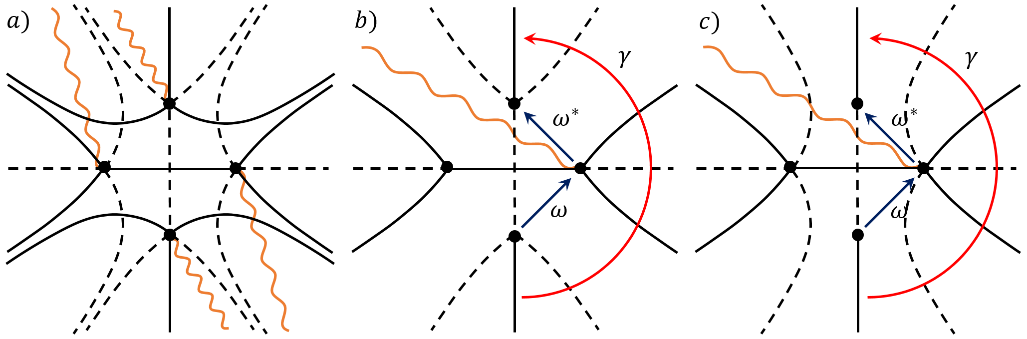
Figure 5: Stokes diagrams for $q(z,E)=\sqrt{z^{4}-E}$; Stokes lines are dashed. (a) A traditional Stokes diagram; dots mark the zeros of the phase integrand. (b) An effective Stokes diagram with a specified path of analytical continuation $\gamma$. (c) An effective Stokes diagram with the same path of analytical continuation but different basepoints.

The main purpose of the effective Stokes diagram is to indicate clearly and transparently what basepoint is used to cross a given Stokes domain. For some values of parameters $\bm{\lambda}$, such diagram can be similar to the traditional one, but for other values the diagrams will differ for sure because effective Stokes line is always emerge from the same basepoint $z_{0}(\bm{\lambda})$ while a traditional one follows the Stokes field. Moreover, effective Stokes diagram is less detailed than the traditional one and may be more convenient for the analysis of complicated equations.

6 Example: the Weber equation

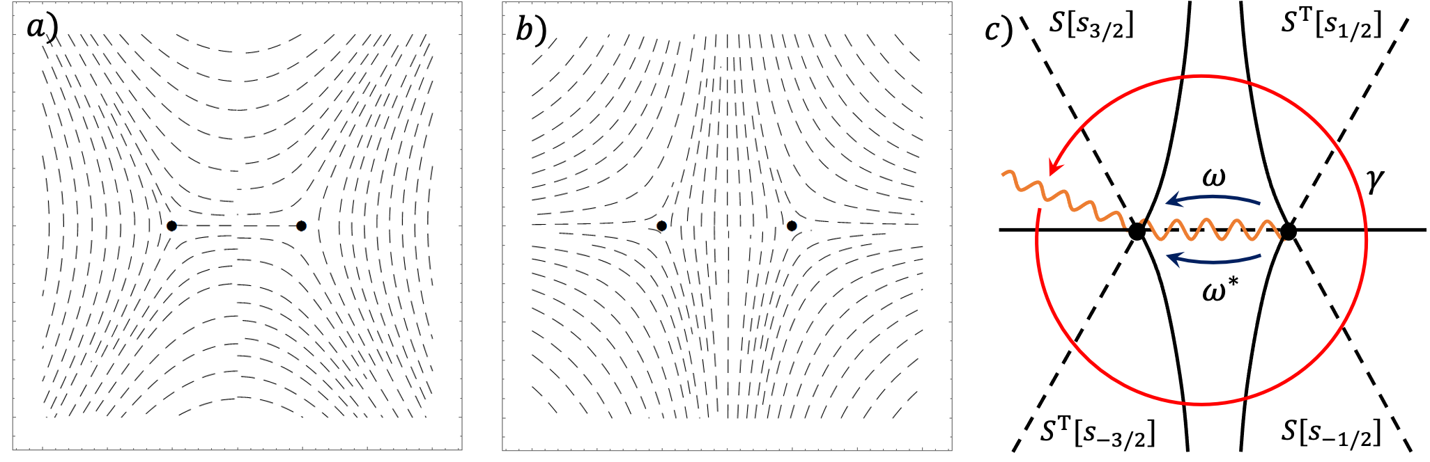
Figure 6: Stokes field (a), anti-Stokes field (b) and an effective Stokes diagram (c) for the Weber equation (20).

We will use WKBJ approximation all throughout this section. Also in this section we will use the symbol $\bm{W}[\omega]\equiv\bm{W}\left[\int_{a}^{b}q(z,\bm{\lambda})\mathrm{d}z\right]\equiv\bm{W}[b,a]$ to underline a value of the phase integral.

Now let us consider the Weber equation

$$\frac{\mathrm{d}^{2}y(z,\delta)}{\mathrm{d}z^{2}}+(z^{2}-\delta^{2})y(z,\delta)=0$$ (20)

with the boundary conditions of a presence of incident wave from the large negative $z$ and an absence of such a wave from the large positive $z$. We define the reflection (transmission) coefficient $\rm{\mathcal{R}}$ ($\rm{\mathcal{T}}$) as a ratio of the amplitudes of the reflected (transmitted) and incident waves. Our aim now is to find these scattering characteristics.

The boundary conditions can be written in terms of $\bm{\psi}$-vectors as

$$\bm{\psi}_{0}=\left(\begin{array}[]{*{2}{c}}1\\ 0\end{array}\right),$$ (21)

where $\bm{\psi}_{0}$ is a $\bm{\psi}$-vector in an anti-Stokes wedge containing a ray $Arg(z)=0$. First of all, scattering characteristics must be written through the Stokes constants. To do this, we must analytically continue our boundary condition (21) to $z$ with $Arg(z)=\pi$. Using Figure 6 and the rules from Section 2, we write

$$\bm{\psi}_{\pi}=\bm{S}\left[s_{3/2}\right]\bm{W}\left[\omega(\delta)\right]\bm{S}^{\mathrm{T}}\left[s_{1/2}\right]\bm{\psi}_{0}\equiv\mathrm{e}^{\mathrm{i}\omega(\delta)}\left(\begin{array}[]{*{2}{c}}1\\ s_{3/2}\end{array}\right),$$ (22)

where $\omega(\delta)=-\mathrm{i}\pi\delta^{2}/2$ is a phase integral calculated above the cut from $z=\delta$ to $z=-\delta$. Now we have to identify incident, reflected and transmitted waves. Since $y_{+}\propto e^{\mathrm{i}z^{2}/2}$ hence it is an outgoing wave for $z\rightarrow+\infty$ as well as for $z\rightarrow-\infty$ and

$$\mathcal{R}=\frac{1}{s_{3/2}},\quad\mathcal{T}=\mathrm{i}\frac{\mathrm{e}^{-\mathrm{i}w}}{s_{3/2}}.$$ (23)

To find $s_{3/2}$, let’s try a traditional method described, for example, in [6, 8]. We can obtain the desired equations for the Stokes constants using a single-valuedness of the general solution and analytically continuing it around the origin far away from the interaction area along the oriented curve $\gamma$ (Figure 6(c)):

$$1=\bm{C}^{2}\bm{S}\left[s_{3/2}\right]\bm{W}\left[\omega\right]\bm{S}^{\mathrm{T}}\left[s_{1/2}\right]\bm{S}\left[s_{-1/2}\right]\bm{W}\left[\omega\right]\bm{S}^{\mathrm{T}}\left[s_{-3/2}\right],$$ (24)

from which follows

$$\begin{cases}s_{1/2}=s_{-3/2}\\ s_{3/2}=s_{-1/2}\\ s_{1/2}s_{3/2}+e^{-2\mathrm{i}w}+1=0.\end{cases}$$ (25)

The $\bm{C}$ operator is squared here because the squared phase integrand $R(z,\bm{\lambda})$ is asymptotic to $z^{2}$ as $z$ goes to complex infinity.

As we can see from the system (25), we cannot find $s_{3/2}$ using the traditional method – we need at least one more restriction for the Stokes constants. In [8] a requirement of the flux conservation is used as the restriction and it gives $s_{-1/2}=-s_{1/2}^{*}$ – it helps to determine the absolute value of the reflection coefficient, but its phase stays unknown. This example shows that even in such a simple situation as the Weber equation, the traditional approach cannot fully resolve the problem.

Actually the flux conservation is a consequence of the real-valuedness and regularity of the coefficients of the Weber equation and hence the same relation can be obtained from the complex conjugation symmetry using (18). Moreover, first two equations from (25) are just a consequence of a symmetry $\{\hat{g}=\mathrm{e}^{\mathrm{i}\pi},\hat{h}=\hat{f}=1\}$ – and it is clear because the symmetry is just a rotation and can be seen even from the usual analytical continuation. Therefore, the only original equation in the system (25) is the last one – it cannot be obtained from any other considerations. But these are not the only consequences of the equation’s symmetries, so let’s write them all.

The first nontrivial symmetry relation can be obtained from the symmetry $\{\hat{g}=\hat{h}=\mathrm{i},\hat{f}=1\}$. It can overlap, for example, Stokes domains associated with $s_{1/2}$ and $s_{-1/2}$. Both of the Stokes constants have the same basepoint $z_{0}(\delta)=\delta$ and $\hat{g}^{-1}z_{0}(\hat{h}\delta)=(-\mathrm{i})\mathrm{i}\delta=\delta$, so

$$\bm{S}\left[s_{1/2}(\mathrm{i}\delta)\right]=\bm{W}\left[\delta,\delta\right]\bm{S}\left[s_{-1/2}(\delta)\right]\bm{W}\left[\delta,\delta\right],$$ (26)

or

$$s_{1/2}(\mathrm{i}\delta)=s_{-1/2}(\delta).$$ (27)

Considering (25), we can see now that all four Stokes wedges can be described by only one function as it was mentioned in the Section 4.

Now consider another symmetry $\{\hat{h}=\mathrm{e}^{\mathrm{i}\pi},\hat{g}=\hat{f}=1\}$. As it was written in the Section 4, such a symmetry gives rise to a functional equation, which can help to illuminate a branching structure of the Stokes constant. For definiteness, we will talk about $s_{3/2}$. To understand what to choose as endpoints in the phase integrals in (19), let’s parametrize $\hat{h}$ as $\hat{h}_{cont}(\mu)=\mathrm{e}^{\mathrm{i}\pi\mu}$ and look at Figure 7. For $s_{3/2}$, the basepoint $z_{0}(\delta)=\delta\mathrm{e}^{\mathrm{i}\pi}$, and the question is how it is changing under our transformation. Using Figure 7 we can see that finally it arrives at the point $z=\delta$, but the phase difference between the initial and the final positions matters because it defines an integration path. That is why we have to write $z_{0}(\hat{h}\delta)=\delta\mathrm{e}^{2\mathrm{i}\pi}$ and

$$\bm{S}\left[s_{3/2}(\delta\mathrm{e}^{\mathrm{i}\pi})\right]=\bm{W}\left[-\omega\right]\bm{S}\left[s_{3/2}(\delta)\right]\bm{W}\left[\omega\right],$$ (28)

or

$$s_{3/2}(\delta\mathrm{e}^{\mathrm{i}\pi})=s_{3/2}(\delta)\mathrm{e}^{-2\mathrm{i}\omega}=s_{3/2}(\delta)e^{-\pi\delta^{2}}.$$ (29)

This functional equation can be solved by substitution $s_{3/2}(\delta)=\mathrm{i}\delta^{\mathrm{i}\delta^{2}}f(\delta^{2})$, where $f(\delta^{2})$ is single-valued in a sense $f(x)=f(x\mathrm{e}^{2\mathrm{i}\pi})$.

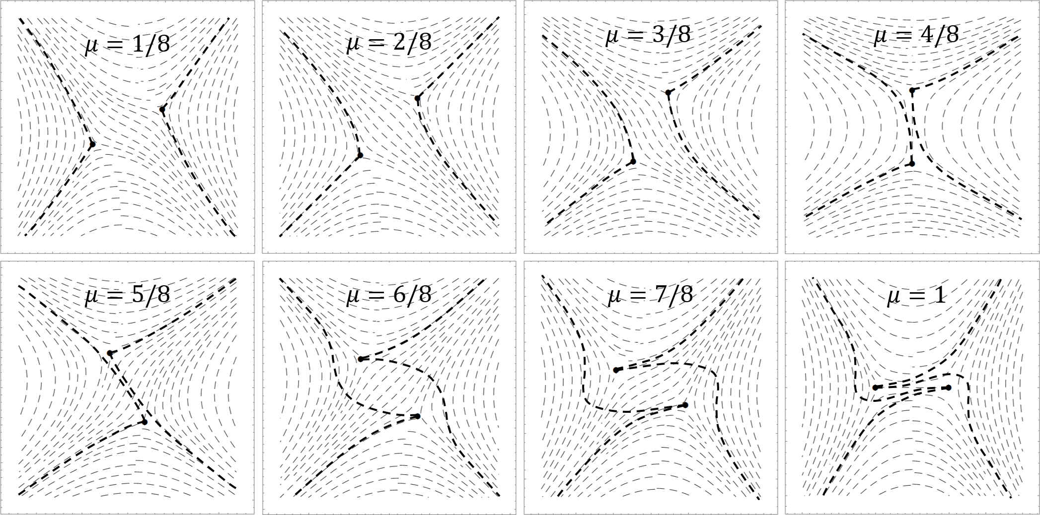
Figure 7: Evolution of the Stokes field and effective Stokes lines under the continuous parameter’s transformation $\hat{h}_{cont}(\mu)=\mathrm{e}^{\mathrm{i}\pi\mu}$.

And, finally, consider a conjugation symmetry $\hat{f}=\hat{g}=\hat{h}=c.c.$. This symmetry relates the Stokes constants in the upper half of the complex plane to the constants in the lower half. In particular, according to (18),

$$\bm{S}\left[-s_{1/2}^{*}(\delta^{*})\right]=\bm{W}\left[z_{0}^{*}(\delta^{*}),\tilde{z}_{0}(\delta)\right]\bm{S}\left[s_{-1/2}(\delta)\right]\bm{W}\left[\tilde{z}_{0}(\delta),z_{0}^{*}(\delta^{*})\right],$$ (30)

and, since $z_{0}(\delta)=\tilde{z}_{0}(\delta)=\delta$,

$$s_{1/2}^{*}(\delta^{*})=-s_{-1/2}(\delta).$$ (31)

For real values of $\delta$ the last relation is nothing but the law of the flux conservation mentioned above. But, for complex values, together with (29) and (25) it gives

$$s_{3/2}(\delta)=s_{-1/2}(\delta)=\mathrm{i}(\mathrm{i}\delta^{2})^{\mathrm{i}\delta^{2}/2}p(\mathrm{i}\delta^{2}),$$ (32)

where $p(x)=p(x\mathrm{e}^{2\mathrm{i}\pi})$ and $p(x)$ is real on the real axis. Now, using (27) and the last equation from the system (25), we can write a functional equation for $p(x)$:

$$p(x)p(-x)=2\cos(\pi x/2).$$ (33)

This functional equation is similar to the Euler’s reflection formula [28] and can be reduced to the formula by substitutions $p(x)=u(x)\sqrt{2\pi}/\Gamma(1/2+x/2)$ and $x=1-2t$, where $u(x)u(-x)=1$. The function $u(x)$ can be found from the boundary conditions of (33). Indeed, we know exactly [8] that $s_{3/2}(0)=\mathrm{i}\sqrt{2}$. We also can assume, according to the approximation of isolated singularities [8, 25], that every Stokes constant approaches an imaginary unit as $\delta$ goes to plus infinity. Taking into consideration (32), we can say that

$$\begin{cases}p(0)=\sqrt{2}\\ p(x)\sim x^{-x/2}\ as\ x\rightarrow\pm\mathrm{i}\infty.\end{cases}$$ (34)

Using the asymptotics of gamma function and definition of $u(x)$, we can finally write that $u(x)=(2\mathrm{e})^{-x/2}$ and

$$s_{3/2}(\delta)=\mathrm{i}(\mathrm{i}\delta^{2})^{\mathrm{i}\delta^{2}/2}\frac{\sqrt{2\pi}(2\mathrm{e})^{-\mathrm{i}\delta^{2}/2}}{\Gamma(1/2+\mathrm{i}\delta^{2}/2)}.$$ (35)

This is an exact expression for the effective Stokes constant for the Weber problem – it can be verified using an exact solution of (20) as it was done in [25]. Now the desired scattering characteristics (23) can be found.

7 Discussion on the possible generalizations

The symmetry relation (15) for connection matrices presented in Section 3 was obtained for the case of the second-order differential equation, but appears to be much more general. In the present section we discuss the range of its applicability.

Consider an arbitrary order system of the first order linear ordinary differential equations:

$$\frac{\mathrm{d}}{\mathrm{d}z}\bm{y}(z,\bm{\lambda})=\bm{M}(z,\bm{\lambda})\bm{y}(z,\bm{\lambda}),$$ (36)

where $\bm{y}$ is a vector of functions to determine and $\bm{M}(z,\bm{\lambda})$ is a square matrix of corresponding dimension. Assume we can write an approximate phase-integral local solution of (36) in the way similar to the case of the second-order equation (1):

$$\bm{y}(z,\bm{\lambda}) \sim\bm{c}\cdot\bm{\tilde{y}}(z,\bm{\lambda}),$$ (37a)

$$\bm{\tilde{y}}_{i}(z,\bm{\lambda}) =\bm{A}_{i}(z,\bm{\lambda})\exp[\mathrm{i}\omega_{i}(z,\bm{\lambda})],$$ (37b)

$$\omega_{i}(z,\bm{\lambda}) =\int_{(z_{0})}^{z}q_{i}(z,\bm{\lambda})\mathrm{d}z,$$ (37c)

where $\bm{A}_{i}$ is a polarization vector, $\bm{c}$ is a vector of coefficients (analogue of $c_{\pm}$), $\bm{\tilde{y}}$ is a vector of approximate phase-integral solutions (37b) (analogue of $y_{\pm}$), and ’$\cdot$’ stands for their inner product. Then, introducing F-matrix and defining symmetry completely analogous to Section 2 and Section 3, we can exploit exactly the same reasoning and arrive to exactly the same symmetry relation with the only one difference: aside from changing basepoint and reordering of the set of the base functions, we have to multiply each function $\bm{\tilde{y}}_{i}$ by an appropriate constant $a_{i}$; the constant was insignificant for the previous discussion because $y_{\pm}$ from (2b) would have been multiplied by the same constant $a=a_{+}=a_{-}$. In the general case considered here the multiplication must be described by a diagonal matrix $\bm{\mathit{\Lambda}}$ such that $\bm{\mathit{\Lambda}}_{ii}=a_{i}$, i.e. the generalization of the symmetry relation (15) takes the form

$$\bm{\mathit{\Lambda}}^{-1}\bm{P}_{\sigma}^{-1}\left\{\hat{f}\bm{F}_{\bm{q},z_{0}}\left[\hat{g}\gamma,\hat{h}\bm{\lambda}\right]\right\}\bm{P}_{\sigma}\bm{\mathit{\Lambda}}$$ (38)

$$\qquad=\bm{W}\left[\hat{g}^{-1}z_{0}(\hat{h}\bm{\lambda}),\tilde{z}_{0}(\bm{\lambda})\right]\bm{F}_{\bm{q},\tilde{z}_{0}}\left[\gamma,\bm{\lambda}\right]\bm{W}\left[\tilde{z}_{0}(\bm{\lambda}),\hat{g}^{-1}z_{0}(\hat{h}\bm{\lambda})\right],$$

where $\bm{q}$ is a vector of the phase integrands $q_{i}$ and $\bm{W}$ has an appropriate dimension. The diagonal elements of the matrix $\bm{\mathit{\Lambda}}$, as well as an explicit form of the permutation matrix $\bm{P}_{\sigma}$, can be determined by a direct application of the symmetry transformation to the base functions $\bm{\tilde{y}}_{i}(z,\bm{\lambda})$.

8 Conclusion

The method of phase integrals is a beautiful and powerful method of a linear ordinary differential equations’ asymptotic analysis, but its range of applicability is highly restricted to relatively simple problems; more complicated problems need additional equations for the Stokes constants. The analysis presented in this paper allows the reader to find functional relations between connection matrices and thus to reduce the number of unknowns.

The main result of the present work is stated by Equation 38. This result, like any other obtained in the paper, is valid for any approximation of the phase-integral type, not only for WKBJ approximation. Furthermore, this result holds not only for the second-order, but also for the arbitrary order system of linear ordinary differential equations.

The symmetry relation (38) and its two-dimensional version (15) are quite general, but not very useful from the practical point of view. To overcome the difficulty, we rewrote the relations in the most common case of the second-order differential equation with use of the limiting form of F-matrix and the concept of effective Stokes constant. The rewritten symmetry relation is stated by Equation 17; we also introduced a concept of effective Stokes diagram which can be a useful tool for the analysis of complicated equations.

We showed that Stokes domains which can be overlapped by the variable transformation $\hat{g}$ are actually associated with the same effective Stokes constant and can be described by the same analytical function. We showed that every differential equation has some formal symmetries (e.g. $\{\hat{h}=\mathrm{e}^{2\mathrm{i}\pi},\hat{g}=\hat{f}=1\}$) which may lead to nontrivial relations for the Stokes constants. We also showed that the symmetry relations allow the reader to write functional equations for the effective Stokes constants; such functional equations help to illuminate a branching structure of the effective Stokes constant and write it as a new single-valued function multiplied by the known multivalued one.

The functional relations which can be obtained from Equation 38 are likely to be as complex as the initial differential equation; however, they are strict and can be used as a basis for the construction of perturbation theory (will be a matter of a separate paper).

Acknowledgments

This work was supported by the Russian Science Foundation (grant No 14-12-01007). The author is grateful to Dr. A. G. Shalashov for careful reading of the manuscript and useful comments.

Appendix A Connection between traditional and
effective Stokes constants

Imagine a Stokes domain with several traditional Stokes lines emerging from the common basepoint. Crossing this domain in terms of the traditional Stokes constants implies multiple sequential applications of either $\bm{S}$ or $\bm{S}^{\mathrm{T}}$ operators. However, as we can see by a direct calculation, Stokes operators $\bm{S}$ as well as $\bm{S}^{\mathrm{T}}$ form a multiplicative group:

$$\bm{S}[s_{2}]\bm{S}[s_{1}]=\bm{S}[s_{2}+s_{1}],\quad\bm{S}^{\mathrm{T}}[s_{2}]\bm{S}^{\mathrm{T}}[s_{1}]=\bm{S}^{\mathrm{T}}[s_{2}+s_{1}].$$ (39)

Consequently, every such set of traditional Stokes constants can be replaced by a single one; the single Stokes constant is just a sum of the traditional constants.

Now consider the reconnection operator $\bm{W}$. As it follows from the properties of the phase integral, these operators also form a multiplicative group:

$$\bm{W}[c,b]\bm{W}[b,a]=\bm{W}[c,a].$$ (40)

And, completely analogous to the situation discussed above, every set of sequential changes of the basepoint can be described by a single reconnection operator.

Finally, imagine a Stokes domain with multiple Stokes lines and multiple basepoints. Crossing this domain in terms of $\bm{S}$ and $\bm{W}$ operators looks like

$$\bm{S}[s_{n}]\bm{W}[a_{n},a_{n-1}]\bm{S}[s_{n-1}]\bm{W}[a_{n-1},a_{n-2}]\ ...\ \bm{S}[s_{1}]\bm{W}[a_{1},a_{0}]\bm{S}[s_{0}].$$ (41)

Note that for any $s^{\prime}$ there is such $s^{\prime\prime}$ that $\bm{S}[s^{\prime}]\bm{W}[b,a]=\bm{W}[b,a]\bm{S}[s^{\prime\prime}]$, therefore we can change the order of $\bm{S}$ and $\bm{W}$ operators. Hence, every such set of operators can always be replaced by a single combination $\bm{S}[s_{l}]\bm{W}[a_{n},a_{0}]$ or, if someone prefers different ordering, $\bm{W}[a_{n},a_{0}]\bm{S}[s_{r}]$. Consequently, every Stokes domain can be described by the effective Stokes constant $s$ despite the number of Stokes lines it contains.

References

- [1] N. Fröman and P. O. Fröman, Physical Problems Solved by the Phase-Integral Method, Cambridge University Press, Cambridge, (2002).
- [2] G. Wentzel, Eine Verallgemeinerung der Quantenbedingungen für die Zwecke der Wellenmechanik, Zeit. f. Phys. 38 (1926) 518.
- [3] H. A. Kramers, Wellenmechanik und halbzahlige Quantisierung, Zeit. f. Phys. 39 (1926) 828.
- [4] L. Brillion, La méchanique ondulatoire de Schrödinger; une méthode générale de résolution par approximations successives, C. R. Acad. Sci. Paris 183 (1926) 24.
- [5] H. Jeffries, On certain approximate solutions of lineae differential equations of the second order, Proc. of London Math. Soc. 23 (1923), 428–436.
- [6] N. Fröman, P. O. Fröman, and B. Lundborg, The Stokes constants for a cluster of transition points, Math. Proc. Cambridge Philos. Soc. 104 (1988), 153–179.
- [7] G. G. Stokes, On the discontinuity of arbitrary constants which appear in divergent developments, Trans. Camb. Phil. Soc. 10 (1857) 105.
- [8] R. B. White, Asymptotic Analysis of Differential Equations, Imperial College Press, (2010).
- [9] J. Heading, An Introduction to Phase Integral Methods, Wiley, NY, (1962).
- [10] M. N. Sergeenko, Semiclassical wave equation and exactness of the WKB method, Physical Review A 53 (1996) 3798.
- [11] M. N. Sergeenko, Zeroth WKB approximation in quantum mechanics, arXiv:quant-ph/0206179.
- [12] A. N. F. Aleixo, et al, Barrier penetration for supersymmetric shape-invariant potentials, J. Phys. A: Math. Gen. 33 (2000) 1503.
- [13] G. Esposito and P. Santorelli, On the phase-integral method for the radial Dirac equation, J. Phys. A: Math. Theor. 42 (2009) 395203.
- [14] E. D. Gospodchikov, A. G. Kutlin, and A. G. Shalashov, Plasma heating and coupling of electromagnetic waves near the upper-hybrid resonance in high- devices, Plasma Phys. Control. Fusion. 59 (2017), no. 6, 06500.
- [15] A. G. Kutlin, E. D. Gospodchikov, and A. G. Shalashov, Linear coupling of the fast extraordinary wave to electrostatic plasma oscillations: a revised theory, accepted for publishing in Physics of Plasmas 12-Oct-2017.
- [16] A. G. Shalashov and E. D. Gospodchikov, Linear coupling of electromagnetic waves in gyrotropic media, Phys. Review E 78 (2008) 065602.
- [17] A. G. Shalashov and E. D. Gospodchikov, On the O-X mode coupling in 3D sheared magnetic field, Plasma Phys. Control. Fusion 52 (2010) 115001.
- [18] A. G. Shalashov and E. D. Gospodchikov, On the structure of Maxwell’s equations in the region of linear coupling of electromagnetic waves in weakly inhomogeneous anisotropic and gyrotropic media, Phys. Usp. 55 (2012), 147–160.
- [19] A. K. Kashani-Poor, Quantization condition from exact WKB for difference equations, J. High Energ. Phys. 2016:180.
- [20] N. Andersson and S. Linnaeus, Quasinormal modes of a Schwarzschild black hole: Improved phase-integral treatment, Phys. Rev. D 46 (1992) 4179.
- [21] Y. Manor, Caustics and energy flux in general relativity, J. Phys. A: Math. Gen. 10 (1977) 765.
- [22] C. Rojas and V. M. Villalba, Computation of inflationary cosmological perturbations in the power-law inflationary model using the phase-integral method, Phys. Rev. D 75 (2007) 063518.
- [23] R. B. Dingle, Asymmpotic Expansions: Their Derivation and Interpretation, Academic Press, London and New York, (1973).
- [24] M. V. Berry, Asymmpotics, superasymptotics, hyperasymptotics, in: Asymptotics Beyond All Orders, H. Segur et al (eds.), Plenum Press, NY, (1991).
- [25] R. B. White and A. G. Kutlin, Bound state energies using phase integral analysis, arXiv:quant-ph/1704.01170.
- [26] E. Delabaere, H. Dillinger, and F. Pham, Exact semiclassical expansions for one-dimensional quantum oscillators, J. Math. Phys. 38 (1997) 6126.
- [27] N. Fröman, P. O. Fröman, and B. Lundborg, Symmetry relations for connection matrices in the phase-integral method, Math. Proc. Camb. Phil. Soc. 104 (1988), 181–191.
- [28] M. Abramowitz and I. A. Stegun, eds., Handbook of Mathematical Functions With Formulas, Graphs, and Mathematical Tables, NBS Applied Mathematics Series 55, National Bureau of Standards, Washington, DC, (1964).