Hybrid Vector Perturbation Precoding: The Blessing of Approximate Message Passing

Abstract

Vector perturbation (VP) precoding is a promising technique for multiuser communication systems operating in the downlink. In this work, we introduce a hybrid framework to improve the performance of lattice reduction (LR) aided precoding in VP. First, we perform a simple precoding using zero forcing (ZF) or successive interference cancellation (SIC) based on a reduced lattice basis. Since the signal space after LR-ZF or LR-SIC precoding can be shown to be bounded to a small range, then along with sufficient orthogonality of the lattice basis guaranteed by LR, they collectively pave the way for the subsequent application of an approximate message passing (AMP) algorithm, which further boosts the performance of any suboptimal precoder. Our work shows that the AMP algorithm can be beneficial for a lattice decoding problem whose data symbols lie in integers $\mathbb{Z}$ and entries of the lattice basis may bot be i.i.d. Gaussian. Numerical results confirm the low-complexity AMP algorithm can improve the symbol error rate (SER) performance of LR aided precoding significantly. Lastly, the hybrid scheme is also proved effective when solving the data detection problem of massive MIMO systems without using LR.

I Introduction

The broadband mobile internet of the next generation is expected to deliver high volume data to a large number of users simultaneously. To meet this demand in the multiuser broadcast network, it is desirable to precode the transmit symbols according to the channel state information (CSI) with improved time-efficiency while retaining the reliability. It is known that precoding by using plain channel inversion performs poorly at all singal-to-noise ratios (SNRs), and further regularization cannot improve the performance substantially. To enhance the throughput, a precoding scheme called vector perturbation (VP) was introduced in [1, 2]. The scheme is based on Tomlinson-Harashima precoding which perturbs the transmitted data by modulo-lattice operations, and it can achieve near-sum-capacity of the system without using dirty-paper techniques [1, 2]. The optimization target of VP requires to solve the closest vector problem (CVP) in a lattice, which has been proved NP-complete by a reduction from the decision version of CVP [3]. Due to the NP-complete nature of the problem, finding its exact solution using sphere decoding [4] (referred to as sphere precoding in [1, 2]) incurs a prohibitive computational complexity that grows exponentially with the dimension of the problem. Therefore, reduced-complexity alternatives providing near-optimal performance must suffice.

Several reduced-complexity precoding algorithms have been proposed in the literature [5, 6, 7, 8, 9, 10, 11]. These algorithms are split into two categories based on whether lattice reduction has been used as pre-processing. In the first category [5, 6, 7, 11, 9], decoding of CVP is solved on the original input basis, and the advantages of low complexity is due to the constraints imposed on the signal space (c.f. [6, 7]) or the lattice basis (c.f. [5, 9]). There is however no theoretical performance guarantee for these simplified methods, so we have to resort to approaches in the second category [8, 12, 13]. These approaches are referred to as lattice reduction (LR) aided precoding (decoding), which consists of lattice reduction as pre-processing and approximated decoding using zero-forcing (ZF), successive interference cancellation (SIC) or other variants. Thanks to the good properties of a reduced basis, approximated decoding based on it has been shown to achieve full diversity order [13, 8]. Compared to algorithms in the first category, the pre-processing complexity of reducing a lattice basis varies from being polynomial to exponential (cf. [14, 15]). This cost is however not an issue [13] in slow-fading channels where the lattice basis is fixed during a large number of time slots, because the lattice basis is only reduced once to serve all the CVP instances.

Focusing on the framework with LR, the aim of this paper is to design a low-complexity message passing algorithm after the phase of approximated decoding. The fundamental principle of message passing algorithms is to decompose high-dimensional problems into sets of smaller low-dimensional problems. This decomposition is often interpreted in a bipartite graph, where the problem variables and factors are represented by graph vertices and dependencies between them represented by edges. Exact message passing methods such as belief propagation (BP) [16, 17] exploit this graphical structure to perform optimization in an iterative manner. By simplifying BP, a new class of low-complexity iterative algorithms referred to as AMP was proposed in [18, 19], and rigorous justification on their performance can be found in [20, 21].

Inspired by the applications [22, 23, 24, 25] of approximate message passing (AMP) [18, 19] in data detection of massive multiple-input multiple-output (MIMO) systems, we investigate a general issue of how to use AMP to solve CVP. By saying general, we emphasize that the data symbols to be estimated in message passing reside in integers $\mathbb{Z}$ which are infinite. As Bayati and Montanari [20] had mentioned their state evolution analysis of AMP can extend beyond compressed sensing (to linear estimation and multi-user detection), we may wonder why AMP cannot be adopted for CVP in a straightforward manner. Actually, even assuming the data symbols are only taken from a finite discrete constellation already complicates the problem of using AMP. For instance, [22] showed that the channel matrix has to become extremely tall as the size the the constellation grows, and [23] argued that the calculation of the posterior mean function of AMP becomes numerically unstable for small values of noise variance. We also noticed that the posterior mean function (denoted as threshold function in [20]) is not Lipschitz continuous for small values of noise variance, so the theoretical justification of AMP does not hold in this scenario (c.f. [20, Section 2.3]). Although we may bypass these issues by using Gaussian distributions as mismatched data distributions, as used in [26, 23, 24, 25], it is easily recognized that their performance is no better than that of Linear Minimum Mean Square Error (LMMSE) estimation. To embrace the low-complexity advantage of AMP and to address the aforementioned issues, it motivates us to design a new decoding architecture for CVP. The key results and contributions of our work are summarized as follows.

1) We propose a hybrid precoding scheme, which uses AMP in conjunction with a sub-optimal estimator after lattice reduction. Considering the theoretical properties and practical performance, we choose the sub-optimal estimator as ZF or SIC, and set the lattice reduction methods as boosted versions of Lenstra–Lenstra–Lov sz (b-LLL) or Korkine-Zolotarev (b-KZ) [14, 27, 15]. After that, we analyze the energy efficiency of precoding with LR-ZF/LR-SIC. On the basis of the proved upper bounds on the energy efficiency, we can deduce upper bounds for the range of data symbols to be estimated by AMP. Since these bounds are derived from a worst case analysis, we also study their empirical distributions.

2) As a reduced lattice basis may not have uniform power in all the columns, we use the approximation techniques in [28, 29] to derive the corresponding AMP algorithm based on simplifying BP. The underlying state evolution equation of it is derived. Subsequently we propose to use ternary distributions and Gaussian distributions for the threshold functions in AMP, whose posterior mean and variance functions have closed-form expressions. The impacts of a reduced basis and parameters in the chosen prior distributions are studied based on the state evolution equation. Simulation results reveal that concatenating AMP to LR-ZF/LR-SIC can provide significant performance improvements.

3) After solving the underlying CVP in VP, the corresponding CVP in massive MIMO can also be solved in an easier manner. Specifically, the lattice bases (channel matrices) in the uplink data detection problem of massive MIMO systems are naturally short and orthogonal, so it suggests we can apply the hybrid scheme to this scenario without using lattice reduction. Simulation results confirm the effectiveness of this extension.

The rest of this paper is organized as follows. We review some basic concepts about lattices and VP in Section II. The hybrid scheme is explained in Section III, which includes demonstrations about why we have reached another problem with a finite constellation size. Section IV presents our AMP algorithm. Simulation results for VP are given in Section VI. The extension to massive MIMO is presented in Section VII, and the last section concludes this paper.

Notations: Matrices and column vectors are denoted by uppercase and lowercase boldface letters. We use $\mathbb{R}$ and $\mathbb{Z}$ to represent the field of real numbers and the ring of rational integers, respectively. $\mathrm{GL}_{n}\left(\mathbb{Z}\right)$ refers to a general linear group with entries in $\mathbb{Z}$. $\lfloor\cdot\rceil$, $|\cdot|$ and $\left\|\cdot\right\|$ respectively refer to (element-wise) rounding, taking the absolute value, and taking the Euclidean norm. $H_{i,j}$ denotes the $(i,j)$th entry of matrix $\mathbf{H}$. $\mathbf{H}^{\top}$ and $\mathbf{H}^{\dagger}=\left(\mathbf{H}^{\top}\mathbf{H}\right)^{-1}\mathbf{H}^{\top}$ denote the transpose and the Moore-Penrose pseudo-inverse of $\mathbf{H}$, respectively. $\mathrm{span}(\mathbf{S})$ denotes the vector space spanned by $\mathbf{S}$. $\pi_{\mathbf{S}}(\mathbf{x})$ and $\pi_{\mathbf{S}}^{\bot}(\mathbf{x})$ denote the projection of $\mathbf{x}$ onto $\mathrm{span}(\mathbf{S})$ and the orthogonal complement of $\mathrm{span}(\mathbf{S})$, respectively. $\propto$ stands for equality up to a normalization constant. $[n]$ denotes $\left\{1,\ldots\thinspace,n\right\}$, $\langle\mathbf{x}\rangle=\sum_{j=1}^{n}x_{j}/n$. $\mathrm{N}(\mu,\Sigma)$ represents a multivariate normal distribution with mean $\mu$ and covariance matrix $\Sigma$. We use the standard asymptotic notation $p(x)=O(q(x))$ when $\lim\sup_{x\rightarrow\infty}|p(x)/q(x)|<\infty$.

II Preliminaries

II-A Lattices

An $n$-dimensional lattice is a discrete additive subgroup in $\mathbb{R}^{n}$. A $\mathbb{Z}$-lattice with basis $\mathbf{H}=[\mathbf{h}_{1},\ldots\thinspace,\mathbf{h}_{n}]\in\mathbb{R}^{m\times n}$ can be represented by

$$\mathcal{L}(\mathbf{H})=\left\{\mathbf{v}\mid\mathbf{v}=\sum_{i\in[n]}c_{i}\mathbf{h}_{i},\thinspace c_{i}\in\mathbb{Z}\right\}.$$

It is necessary to know whether the basis vectors $\mathbf{h}_{i}$’s are short and nearly orthogonal. This property can be measured by the orthogonality defect (OD):

$$\xi(\mathbf{H})=\frac{\prod_{i=1}^{n}\left\|\mathbf{h}_{i}\right\|}{\sqrt{\det(\mathbf{H}^{\top}\mathbf{H})}}.$$ (1)

We have $\xi(\mathbf{H})\geq 1$ due to Hadamard’s inequality. Given $\mathbf{H}$, the denominator of (1) is fixed, while the $\left\|\mathbf{h}_{i}\right\|$ in the numerator can be reduced to get close to the $i$th successive minimum of $\mathcal{L}(\mathbf{H})$, which is defined by the smallest real number $r$ such that $\mathcal{L}(\mathbf{H})$ contains $i$ linearly independent vectors of length at most $r$:

$$\lambda_{i}(\mathbf{H})=\inf\left\{r\mid\dim(\mathrm{span}((\mathcal{L}\cap\mathcal{B}(\mathbf{0},r)))\geq i\right\},$$

in which $\mathcal{B}(\mathbf{0},r)$ denotes a ball centered at the origin with radius $r$.

The goal of lattice reduction is to find, for a given lattice, a basis matrix with favorable properties. There are many well developed reduction algorithms. Here we review the polynomial time LLL [14] reduction and the exponential time KZ [27] reduction, followed by their boosted variants.

Definition 1 ([14]).

A basis $\mathbf{H}$ is called LLL reduced if it satisfies the size reduction conditions of $|R_{i,j}/R_{i,i}|\leq\frac{1}{2}$ for $1\leq i\leq n$, $j>i$, and Lov sz’s conditions of $\delta R_{i,i}^{2}\leq R_{i,i+1}^{2}+R_{i+1,i+1}^{2}$ for $1\leq i\leq n-1$.

In the definition, $R_{i,j}$’s refer to elements of the $\mathbf{R}$ matrix of the QR decomposition on $\mathbf{H}$, and $\delta\in(1/4,1)$ is called Lov sz’s constant. Define $\beta=1/\sqrt{\delta-1/4}\in(2/\sqrt{3},\infty)$, for an LLL reduced basis $\mathbf{H}$ we have [14]

$$\xi(\mathbf{H})\leq\beta^{n(n-1)/2}.$$ (2)

Definition 2 ([30]).

A basis $\mathbf{H}$ is called KZ reduced if it satisfies the size reduction conditions, and the projection conditions of $\pi_{\left[\mathbf{h}_{1},\ldots\thinspace,\mathbf{h}_{i-1}\right]}^{\perp}(\mathbf{h}_{i})$ being the shortest vector of the projected lattice $\pi_{\left[\mathbf{h}_{1},\ldots\thinspace,\mathbf{h}_{i-1}\right]}^{\perp}([\mathbf{h}_{i},\ldots\thinspace,\mathbf{h}_{n}])$ for $1\leq i\leq n$.

If $\mathbf{H}$ is KZ reduced, we have [30]

$$\xi(\mathbf{H})\leq\left(\prod_{i=1}^{n}\frac{\sqrt{i+3}}{2}\right)\left(\frac{2n}{3}\right)^{n/2}.$$ (3)

In this paper we will adopt the boosted version of LLL/KZ so as to get shorter and more orthogonal basis vectors [15] .

Definition 3 ([15]).

A basis $\mathbf{H}$ is called boosted LLL (b-LLL) reduced if it satisfies diagonal reduction conditions of $\delta R_{i,i}^{2}\leq(R_{i,i+1}-\lfloor R_{i,i+1}/R_{i,i}\rceil R_{i,i})^{2}+R_{i+1,i+1}^{2}$ for $1\leq i\leq n-1$, and all $\mathbf{h}_{i}$ for $2\leq i\leq n$ are reduced by an approximate CVP oracle with list size $p$ along with a rejection operation.

Although the definition of b-LLL ensures that it performs no worse than LLL in reducing the lengths of basis vectors, only the same bound on OD has been proved: $\xi(\mathbf{H})\leq\beta^{n(n-1)/2}$ [15].

Definition 4 ([15]).

A basis $\mathbf{H}$ is called boosted KZ (b-KZ) reduced if it satisfies the projection conditions as KZ, and the length reduction conditions of $\left\|\mathbf{h}_{i}\right\|\leq\left\|\mathbf{h}_{i}-\mathcal{Q}_{\mathcal{L}(\left[\mathbf{h}_{1},\ldots\thinspace,\mathbf{h}_{i-1}\right])}(\pi_{\left[\mathbf{h}_{1},\ldots\thinspace,\mathbf{h}_{i-1}\right]}(\mathbf{h}_{i}))\right\|$ for $2\leq i\leq n$, where $\mathcal{Q}_{\mathcal{L}(\left[\mathbf{h}_{1},\ldots\thinspace,\mathbf{h}_{i-1}\right])}\left(\cdot\right)$ is the nearest neighbor quantizer w.r.t. $\mathcal{L}(\left[\mathbf{h}_{1},\ldots\thinspace,\mathbf{h}_{i-1}\right])$.

If $\mathbf{H}$ is b-KZ reduced, we have

$$\xi(\mathbf{H})\leq\frac{\sqrt{n}}{2}\left(\prod_{i=1}^{n-1}\frac{\sqrt{i+3}}{2}\right)\left(\frac{2n}{3}\right)^{n/2}.$$ (4)

II-B Vector Perturbation and CVP

Vector perturbation is a non-linear precoding technique that aims to minimize the transmitted power that is associated with the transmission of a certain data vector [1, 2]. Assume the base station is equipped with $m$ transmit antennas to broadcast messages to $n$ individual users, and each user has only one antenna. The observed signals at users $1$ to $n$ can be collectively expressed as as a vector:

$$\bar{\mathbf{t}}=\mathbf{B}\mathbf{t}+\bar{\mathbf{w}}$$ (5)

where $\mathbf{B}\in\mathbb{R}^{n\times m}$ denotes a channel matrix whose entries admit $\mathrm{N}(0,1)$, $\mathbf{t}\in\mathbb{R}^{m}$ is a transmitted signal, and $\bar{\mathbf{w}}\sim\mathrm{N}(\mathbf{0},\sigma_{w}^{2}\mathbf{I}_{n})$ denotes additive Gaussian noise.

With perfect channel knowledge at the base station, the transmitted signal $\mathbf{t}$ is designed to be a truncation of the channel inversion precoding $\mathbf{B}^{\dagger}\mathbf{s}$:

$$\mathbf{t}=\mathbf{B}^{\dagger}(\mathbf{s}-M\mathbf{x}),$$ (6)

where $\mathbf{x}\in\mathbb{Z}^{n}$ is an integer vector to be optimized, $\mathbf{s}\in\mathcal{M}^{n}$ is the symbol vector. We set the constellation as $\mathcal{M}=\{0,\ldots,M-1\}$ where $M>1$ is a positive integer. All quadrature amplitude modulation (QAM) constellations can be transformed to this format after adjusting (6).

Assume the transmitted signal has unit power, and let $E_{\mathbf{t}}\triangleq\left\|\mathbf{t}\right\|$ be a normalization factor. Then the signal vector at users is represented by

$$\bar{\mathbf{t}}=(\mathbf{s}-M\mathbf{x})/E_{\mathbf{t}}+\bar{\mathbf{w}}.$$ (7)

Let $\bar{\mathbf{t}}^{\prime}=E_{\mathbf{t}}\bar{\mathbf{t}}$, $\bar{\mathbf{w}}^{\prime}=E_{\mathbf{t}}\bar{\mathbf{w}}$, since $M\mathbf{x}\thinspace\mod\thinspace M=\mathbf{0}$, the above equation can be transformed to

$$\lfloor\bar{\mathbf{t}}^{\prime}\rceil\thinspace\mod\thinspace M=\lfloor\mathbf{s}+\bar{\mathbf{w}}^{\prime}\rceil\thinspace\mod\thinspace M.$$ (8)

From (8), we can see that if $|\bar{w}_{i}^{\prime}|<\frac{1}{2}$ $\forall\thinspace i$, where $\bar{\mathbf{w}}^{\prime}\in\mathrm{N}(\bm{0},\sigma_{w}^{2}E_{\mathbf{t}}\mathbf{I}_{n})$, then $\mathbf{s}$ can be faithfully recovered.

To decrease the decoding error probability which is dominated by $E_{\mathbf{t}}$, the transmitter has to address the following optimization problem:

$$\arg\min_{\mathbf{x}\in\mathbb{Z}^{n}}\left\|\mathbf{B}^{\dagger}(\mathbf{s}-M\mathbf{x})\right\|^{2}.$$ (9)

Define $\mathbf{y}=\mathbf{B}^{\dagger}\mathbf{s}\in\mathbb{R}^{m}$, $\mathbf{H}=M\mathbf{B}^{\dagger}\in\mathbb{R}^{m\times n}$, then (9) represents a CVP instance of lattice decoding:

$$\mathbf{x}^{\mathrm{cvp}}=\arg\min_{\mathbf{x}\in\mathbb{Z}^{n}}\left\|\mathbf{y}-\mathbf{H}\mathbf{x}\right\|^{2}.$$ (10)

This CVP is different from the CVP in MIMO detection because the distance distribution from $\mathbf{y}$ to lattice $\mathcal{L}(\mathbf{H})$ is not known, the lattice basis is the inverse of the channel matrix that has highly correlated entries, and the data symbols are optimized over $\mathbb{Z}^{n}$ rather than over a small finite constellation.

III The hybrid precoding scheme

Our hybrid precoding scheme to solve the CVP in (10) consists of two phases:

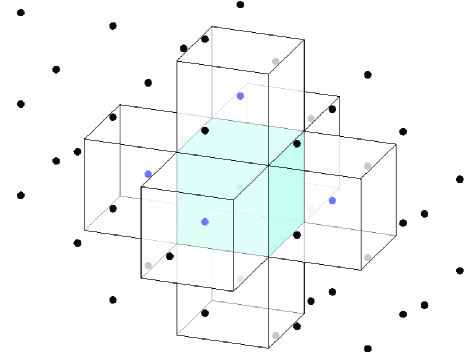
Figure 1: Exploring the vicinity of a good candidate $\mathbf{x}^{\mathrm{zf}}\in\mathbb{R}^{3}$, whose decision parallelepiped is the cyan cube. After updating the target vector $\mathbf{y\leftarrow y}-\mathbf{H}\mathbf{x}^{\mathrm{zf}}$, to optimize $\min_{\mathbf{x}\in\left\{-1,0,1\right\}^{3}}\left\|\mathbf{y}-\mathbf{H}\mathbf{x}\right\|$ enables locating all the blue lattice points inside the white cubes.

Phase 1 (approximated decoding): Apply lattice reduction to the input basis to get $\mathbf{H}\leftarrow\mathbf{H}\mathbf{U}$, where $\mathbf{U}\in\mathrm{GL}_{n}(\mathbb{Z})$ is induced by the reduction operation. Based on the reduced $\mathbf{H}$, use ZF or SIC to get a sub-optimal candidate: $\hat{\mathbf{x}}=\mathbf{x}^{\mathrm{zf}}$ or $\hat{\mathbf{x}}=\mathbf{x}^{\mathrm{sic}}$.

Phase 2 (AMP decoding): Let $\mathbf{y}\leftarrow\mathbf{y}-\mathbf{H}\hat{\mathbf{x}}$ and define a finite constraint $\mathcal{B}=\left\{-B,-B+1,\ldots,B-1,B\right\}$. After that, use an AMP algorithm to solve:

$$\mathbf{x}^{\mathrm{amp}}=\arg\min_{\mathbf{x}\in\mathcal{B}^{n}}\left\|\mathbf{y}-\mathbf{H}\mathbf{x}\right\|^{2}.$$ (11)

Lastly return $\hat{\mathbf{x}}+\mathbf{x}^{\mathrm{amp}}$.

The underlying rationale is demonstrated in Fig. 1. Regarding the algorithmic routines in Phase 1, $\mathbf{x}^{\mathrm{zf}}=\lfloor\mathbf{H}^{\dagger}\mathbf{y}\rceil$, and we refer to [31, 15] for those of lattice reduction, to [32] for that of $\mathbf{x}^{\mathrm{sic}}$.

To ensure the hybrid decoding scheme is correct and efficient, the following two issues are addressed in the paper.

• Regarding the transformation from (10) to (11), one has to specify a minimum range for constraint $\mathcal{B}^{n}$ such that

  $$\arg\min_{\mathbf{x}\in\mathcal{B}^{n}}\left\|\mathbf{y}-\mathbf{H}\hat{\mathbf{x}}-\mathbf{H}\mathbf{x}\right\|^{2}=\arg\min_{\mathbf{x}\in\mathbb{Z}^{n}}\left\|\mathbf{y}-\mathbf{H}\mathbf{x}\right\|^{2}.$$

  Generally speaking, problem (11) becomes easier if $B$ is smaller. In Section III-A, we will examine the theoretical and empirical bounds of constraint $\mathcal{B}^{n}$.

• The AMP algorithms in [18, 19] were assuming at least the entries of $\mathbf{H}$ being sub-Gaussian with variance $O(1/n)$. Can we derive an AMP algorithm that is suitable for problem (11), and possibly the routines are simple and have closed-form expressions? We will first address relevant prerequisites in Section III-B. Considering all the constraints, Section IV will present an AMP algorithm based on simplifying BP.

III-A The bounds of constraint $\mathcal{B}^{n}$

In the application to precoding, we show in this section that the estimation range $\mathcal{B}^{n}$ is bounded after LR-ZF/LR-SIC. Now we introduce a parameter called energy efficiency to describe how far a suboptimal perturbation is from the optimal one.

Definition 5.

The energy efficiency of an algorithm providing $\hat{\mathbf{x}}$ is the smallest $\eta_{n}$ in the constraint

$$\left\|\mathbf{y}-\mathbf{H}\hat{\mathbf{x}}\right\|\leq\eta_{n}\left\|\mathbf{y}-\mathbf{H}\mathbf{x}^{\mathrm{cvp}}\right\|,$$ (12)

where $\mathbf{x}^{\mathrm{cvp}}=\arg\min_{\mathbf{x}\in\mathbb{Z}^{n}}\left\|\mathbf{y}-\mathbf{Hx}\right\|$, and we say this algorithm solves $\eta_{n}$-CVP .

We first analyze the energy efficiency $\eta_{n}$ of b-LLL/b-KZ aided ZF/SIC, and then address the bound for $\mathcal{B}^{n}$ based on $\eta_{n}$ . The reasons for choosing b-LLL/b-KZ as the reduction method are: i) b-LLL provides better practical performance than that of LLL [15], and ii) b-KZ characterizes the theoretical limit of strong (with exponential complexity) LR methods.

Theorem 1.

For the SIC estimator, if the lattice basis is reduced by b-LLL, then

$$\eta_{n}=\beta^{n}/\sqrt{\beta^{2}-1},$$ (13)

where $\beta\in(2/\sqrt{3},\infty)$; and if the basis is reduced by b-KZ, then

$$\eta_{n}=1+\frac{8n}{9}\left(n-1\right)^{1+\ln(n-1)/2}.$$ (14)

Proof:

The proof relies on upper bounding the diagonal entries of $\mathbf{R}$ (the R matrix in the QR factorization of $\mathbf{H}$). Since boosted LLL/KZ has the same diagonal entries as those of LLL/KZ, we can use results about energy efficiency from classic LLL/KZ if they exist. Hence Eq. (13) is adapted from LLL in [8]. As no such result is known for KZ, we prove a sharp bound for both KZ and b-KZ in Appendix B, where the skill involved is essentially due to [33]. ∎

Theorem 2.

For the ZF estimator, if the lattice basis is reduced by b-LLL, then

$$\eta_{n}=2n\prod_{j=1}^{n}\beta^{j-1}+1;$$ (15)

and if the basis is reduced by b-KZ, then

$$\eta_{n}=2n\prod_{j=1}^{n}j^{2+\ln(j)/2}+1.$$ (16)

Proof:

See Appendix C. ∎

Notice that the maximal range of $\mathcal{B}$ is $\max_{i\in n}|\hat{x}_{i}-x_{i}^{\mathrm{cvp}}|$. Here, we upper bound it by a function about the energy efficiency $\eta_{n}$. Denote $\varrho(\mathbf{H})$ as the covering radius of lattice $\mathcal{L}(\mathbf{H})$, it follows from the triangle inequality and $\left\|\mathbf{y}-\mathbf{H}\mathbf{x}^{\mathrm{cvp}}\right\|\leq\varrho(\mathbf{H})$ that

$$\left\|\mathbf{H}\left(\hat{\mathbf{x}}-\mathbf{x}^{\mathrm{cvp}}\right)\right\| \leq\left\|\mathbf{y}-\mathbf{H}\hat{\mathbf{x}}\right\|+\left\|\mathbf{y}-\mathbf{H}\mathbf{x}^{\mathrm{cvp}}\right\|$$

$$\leq\left(\eta_{n}+1\right)\varrho(\mathbf{H}).$$

With unitary transform, we have $\left\|\mathbf{H}\left(\hat{\mathbf{x}}-\mathbf{x}^{\mathrm{cvp}}\right)\right\|=\left\|\mathbf{R}\left(\hat{\mathbf{x}}-\mathbf{x}^{\mathrm{cvp}}\right)\right\|$. To get the upper bound for each $|\hat{x}_{i}-x_{i}^{\mathrm{cvp}}|$, we can expand the quadratic form in the l.h.s. of

$$\left\|\mathbf{R}\left(\hat{\mathbf{x}}-\mathbf{x}^{\mathrm{cvp}}\right)\right\|^{2}\leq\left(\eta_{n}+1\right)^{2}\varrho^{2}(\mathbf{H})$$

to get

$$R_{n,n}^{2}\left(\hat{x}_{n}-x_{n}^{\mathrm{cvp}}\right)^{2}+\cdots+\left(R_{1,1}\left(\hat{x}_{n}-x_{n}^{\mathrm{cvp}}\right)+R_{1,n}\left(\hat{x}_{n}-x_{n}^{\mathrm{cvp}}\right)\right)^{2}$$

$$\leq\left(\eta_{n}+1\right)^{2}\varrho^{2}(\mathbf{H}).$$

For a reduced basis, we know that all the column vectors are short and the diagonal entries are not very small w.r.t. the successive minima: $\left\|\mathbf{h}_{i}\right\|\leq\omega_{i}\lambda_{i}(\mathbf{H})$, $|R_{i,i}|\geq\lambda_{1}(\mathbf{H})/\varpi_{i}$, where the values of $\omega_{i}$ and $\varpi_{i}$ can be found in [15]. Now regarding the bound of $|\hat{x}_{n}-x_{n}^{\mathrm{cvp}}|$, it follows from $R_{n,n}^{2}\left(\hat{x}_{n}-x_{n}^{\mathrm{cvp}}\right)^{2}\leq\left(\eta_{n}+1\right)^{2}\varrho^{2}(\mathbf{H})$ that

$$|\hat{x}_{n}-x_{n}^{\mathrm{cvp}}| \leq\left(\eta_{n}+1\right)\varrho(\mathbf{H})/|R_{n,n}|$$

$$\leq\left(\eta_{n}+1\right)\varrho(\mathbf{H})\varpi_{n}/\lambda_{1}(\mathbf{H}).$$

Similarly for $|\hat{x}_{n-1}-x_{n-1}^{\mathrm{cvp}}|$, one has

$$|\hat{x}_{n-1}-x_{n-1}^{\mathrm{cvp}}| \leq\left\|\mathbf{R}_{:,1:n-1}\left(\hat{\mathbf{x}}_{1:n-1}-\mathbf{x}_{1:n-1}^{\mathrm{cvp}}\right)\right\|/|R_{n-1,n-1}|$$

$$\leq\left(\left(\eta_{n}+1\right)\varrho(\mathbf{H})+\omega_{n}\lambda_{n}(\mathbf{H})|\hat{x}_{n}-x_{n}^{\mathrm{cvp}}|\right)\varpi_{n-1}/\lambda_{1}(\mathbf{H})$$

$$\leq\left(\eta_{n}+1\right)\varpi_{n-1}\varrho(\mathbf{H})/\lambda_{1}(\mathbf{H})$$

$$\thinspace\thinspace\thinspace+\omega_{n}\left(\eta_{n}+1\right)\varpi_{n}\varpi_{n-1}\lambda_{n}(\mathbf{H})\varrho(\mathbf{H})/\lambda_{1}^{2}(\mathbf{H}).$$

By induction, we can obtain the upper bounds of $|\hat{x}_{n-2}-x_{n-2}^{\mathrm{cvp}}|,\ldots\thinspace,|\hat{x}_{1}-x_{1}^{\mathrm{cvp}}|$. The concrete values of these bounds can be evaluated by using the values of $\eta_{i}$, $\omega_{i}$ and $\varpi_{i}$ based on the chosen LR aided ZF/SIC algorithms. In summary, the maximal error distance $\max_{i\in n}|\hat{x}_{i}-x_{i}^{\mathrm{cvp}}|$ is a function about $\eta_{n}$ which is finite.

To complement the theoretical analysis above, we further conduct an empirical study to understand the actual distributions of $\hat{x}_{i}-x_{i}^{\mathrm{cvp}}$. We enumerate the possible values of errors and their probabilities using lattice reduction (using boosted LLL) aided ZF/SIC estimators in Table I. Note that these errors are not the decoding error of VP, but they affect the decoding error of VP through resulted SNR. Generally, more evident differences have smaller SNRs. In the setup of the simulation, the probabilities are averaged from $10^{4}$ Monte Carlo runs, the size of constellations is set as $M=32$, and the size of systems are set as $m=n=8,12,16,20$, respectively. Since our simulations show that choosing other values of $M$ still yields similar error distributions as in Table I, we don’t present them in this paper.

TABLE I: The values $\hat{x}_{i}-x_{i}^{\mathrm{cvp}}$ with $i\in[n]$ and their probabilities after “Phase 1” in hybrid precoding.

error	distance	$-4$	$-3$	$-2$	$-1$	$0$	$1$	$2$	$3$	$4$
$n=8$	LR-ZF	$0$	$0$	$0$	$0.0666$	$0.8670$	$0.0664$	$0$	$0$	$0$
	LR-SIC	$0$	$0$	$0.0001$	$0.0505$	$0.8973$	$0.0518$	$0.0001$	$0$	$0$
$n=12$	LR-ZF	$0$	$0$	$0.0001$	$0.0891$	$0.8233$	$0.0875$	$0.0001$	$0$	$0$
	LR-SIC	$0$	$0$	$0.0013$	$0.0817$	$0.8348$	$0.0808$	$0.0013$	$0$	$0$
$n=16$	LR-ZF	$0$	$0$	$0.0006$	$0.1123$	$0.7752$	$0.1112$	$0.0008$	$0$	$0$
	LR-SIC	$0$	$0.0001$	$0.0040$	$0.1113$	$0.7715$	$0.1090$	$0.0039$	$0.0001$	$0$
$n=20$	LR-ZF	$0$	$0.0001$	$0.0022$	$0.1342$	$0.7284$	$0.1327$	$0.0024$	$0.0001$	$0$
	LR-SIC	$0.0001$	$0.0007$	$0.0082$	$0.1348$	$0.7119$	$0.1352$	$0.0086$	$0.0005$	$0$

Table I shows the values of error distance of both LR-ZF and LR-SIC concentrate around $0$. It is clear that the range of $\hat{x}_{i}-x_{i}^{\mathrm{cvp}}$ slowly grows w.r.t. the dimension of the system; however, these values are much smaller than their theoretical upper bounds. The statistical information provided by this empirical study can be taken into account when designing threshold functions for AMP.

III-B Prerequisites for AMP

Regarding the constellation of $\mathbf{x}$, we have demonstrated that the error of ZF/SIC estimator is bounded to a function about system dimension $n$ and some inherent lattice metrics. This means we are not facing an infinite lattice decoding problem with $\mathbb{Z}$ constellations in Eq. (11), whence the application of AMP becomes possible. Moreover, the bound of $\mathcal{B}^{n}$ can be made very small when designing our AMP algorithm.

Regarding the distribution of noise $\mathbf{w}^{\mathrm{amp}}=\mathbf{y}-\mathbf{H}\mathbf{x}$, it is not known a priori. We can equip $\mathbf{w}^{\mathrm{amp}}$ with a Gaussian distribution $\mathrm{N}(\bm{0},\sigma^{2}\mathbf{I}_{m})$ with $0<\sigma^{2}<\left\|\mathbf{y}-\mathbf{H}\hat{\mathbf{x}}\right\|^{2}/m$, based on which we obtain the non-informative likelihood function of $\mathbf{x}$:

$$p(\mathbf{x})\sim\mathrm{N}(\mathbf{H}^{-1}\mathbf{y},\sigma^{2}(\mathbf{H}^{\top}\mathbf{H})^{-1}).$$

Lastly, as for the channel matrix $\mathbf{H}$, if the basis now has i.i.d. entries satisfying $\mathbb{E}H_{i,j}=0$ and $\mathbb{E}H_{i,j}^{2}=1/n$ and admitting sub-Gaussian tail conditions [21, 20], which we refer to as sub-Gaussian conditions, then one can adopt the well developed AMP [18, 28] or GAMP [34] algorithms to solve our problem in Eq. (11) rigorously. On the contrary, if a reduced basis is far from having sub-Gaussian entries, then using AMP cannot provide any performance gain. Fortunately, it is known that a basis is short and nearly orthogonal after lattice reduction, which means its column-wise dependency is small. Moreover, a reduced basis in VP often has “small” entries (in the sense of [35]) such that the approximations in AMP are valid. We further justified the two arguments above in Appendix A. As a result, we propose to describe a reduced basis with Gaussian distributions and implement AMP on it, and the plausibility of this method will be confirmed by simulations. Without loss of generality, suppose $H_{i,j}\sim\mathrm{N}(0,\sigma_{j}^{2}/m)$ for $i\in[m]$, then one can use the values of basis entries to obtain the maximum likelihood estimation for each $\sigma_{j}^{2}$. To see this, note that the likelihood function w.r.t. $\sigma_{j}^{2}$ and $m$ samples $H_{1,j},\ldots,H_{m,j}$ is $L\left(H_{1,j},\ldots,H_{m,j},\sigma_{j}^{2}\right)=$

$$\frac{1}{\left(2\pi\sigma_{j}^{2}/m\right)^{n/2}}\exp\left(-\frac{1}{2\sigma_{j}^{2}/m}\sum_{i\in[m]}H_{i,j}^{2}\right),$$ (17)

then it follows from solving $\partial L\left(H_{1,j},\ldots,H_{m,j},\sigma_{j}^{2}\right)/\partial\sigma_{j}^{2}=0$ that $\sigma_{j}^{2}=\sum_{i\in[m]}H_{i,j}^{2}$. Based on the above, we will modify the AMP algorithm in [18, 28] and analyze its performance in the next section.

IV AMP algorithm for Eq. (11)

Combing the non-informative likelihood function with the prior function $p_{X}(x_{i})$, it yields a Maximum-a-Posteriori (MAP) function for Bayesian estimation:

$$p(\mathbf{x}|\mathbf{y},\mathbf{H})\varpropto\prod_{a\in[m]}p_{a}(\mathbf{x},y_{a})\prod_{i\in[n]}p_{X}(x_{i}),$$ (18)

where $p_{a}(\mathbf{x},y_{a})=\exp(-\frac{1}{2\sigma^{2}}(y_{a}-\mathbf{H}_{a,1:n}\mathbf{x})^{2})$, and $p_{X}(x_{i})$ will be designed in Section V. The factorized structure in (18) can be conveniently described by a factor graph [36, 37]. It includes a variable node for each $x_{i}$, a factor node for each $p_{X}(x_{i})$, and a factor node for each $p_{a}(\mathbf{x},y_{a})$, where $i\in[n]$, $a\in[m]$. If $x_{i}$ appears in $p_{X}(x_{i})$ or $p_{a}(\mathbf{x},y_{a})$, then they are connected by an edge. Clearly, $x_{i}$ and $p_{a}(\mathbf{x},y_{a})$ are connected if and only if and only if $H_{a,i}\neq 0$. Such a factor graph is reproduced in Fig. 2.

In the sequel, we first show how to simplify BP to reach an AMP algorithm by using the approximation techniques in [18, 28, 29]. After that, we will characterize the symbol-wise estimation errors in Theorem 3 and present the threshold functions of certain prior distributions.

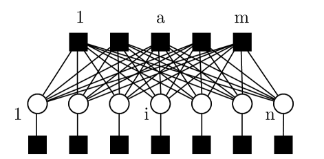
Figure 2: The factor graph associated to the probability distribution (18). Empty circles corresponds to variables, lines correspond to edges, and solid squares correspond to factors.

IV-A Simplified BP

Each factor graph naturally induces a BP algorithm [19] that involves two types of messages: messages from variable nodes to factor nodes denoted by $J_{i\rightarrow a}(x_{i})$, and messages from factor nodes to variable nodes, denoted by $\hat{J}_{a\rightarrow i}(x_{i})$. Here, messages refer to probability distribution functions, which are recursively updated to compute marginal posterior density functions for the variables. At the $t$th iteration, they are updated as follows

$$\hat{J}_{a\rightarrow i}^{t}(x_{i})=\int_{\mathbf{x}\backslash x_{i}}\{p_{a}(\mathbf{x},y_{a})\prod_{j\in[n]\backslash i}J_{j\rightarrow a}^{t}(x_{j})\}\mathrm{d}\mathbf{x},$$ (19)

$$J_{i\rightarrow a}^{t+1}(x_{i})=p_{X}(x_{i})\prod_{b\in[m]\backslash a}\hat{J}_{b\rightarrow i}^{t}(x_{i}).$$ (20)

These messages are impractical to evaluate in the Lebesgue measure space, and thus often simplified by approximation techniques. We make the approximation from an expectation propagation [38] perspective hereby. Suppose the message in Eq. (19) is estimated by a Gaussian function with mean $\alpha_{a\rightarrow i}^{t}/\beta_{a\rightarrow i}^{t}$ and variance $1/\beta_{a\rightarrow i}^{t}$, then

$$\hat{J}_{a\rightarrow i}^{t}(x_{i}) = \mathrm{N}(H_{a,i}x_{i};\alpha_{a\rightarrow i}^{t}/\beta_{a\rightarrow i}^{t},1/\beta_{a\rightarrow i}^{t}).$$ (21)

By substituting Eq. (21) into Eq. (20), we have

$$J_{i\rightarrow a}^{t+1}(x_{i}) \varpropto p_{X}(x_{i})\exp((\sum_{b\in[m]\backslash a}H_{b,i}\alpha_{b\rightarrow i}^{t})x_{i}$$

$$-1/2(\sum_{b\in[m]\backslash a}H_{b,i}^{2}\beta_{b\rightarrow i}^{t})x_{i}^{2}+O(nH_{a,i}^{3}x_{i}^{3}))$$

$$\varpropto p_{X}(x_{i})\mathrm{N}(x_{i};u_{i\rightarrow a},v_{i\rightarrow a}),$$ (22)

where

$$u_{i\rightarrow a}^{t}=\frac{\sum_{b\in[m]\backslash a}H_{b,i}\alpha_{b\rightarrow i}^{t}}{\sum_{b\in[m]\backslash a}H_{b,i}^{2}\beta_{b\rightarrow i}^{t}},$$ (23)

$$v_{i\rightarrow a}^{t}=\frac{1}{\sum_{b\in[m]\backslash a}H_{b,i}^{2}\beta_{b\rightarrow i}^{t}}.$$ (24)

In the other direction, we work out messages $J_{i\rightarrow a}^{t+1}(x_{i})$ with Gaussian functions through matching their first and second order moments by the following constraints:

$$J_{i\rightarrow a}^{t+1}(x_{i})=\mathrm{N}(x_{i};\eta(u_{i\rightarrow a}^{t},v_{i\rightarrow a}^{t}),\mathrm{\kappa}(u_{i\rightarrow a}^{t},v_{i\rightarrow a}^{t})),$$ (25)

$$\mathrm{\eta}(u_{i\rightarrow a}^{t},v_{i\rightarrow a}^{t})=\int_{x}xp_{X}(x)\mathrm{N}(x;\thinspace u_{i\rightarrow a}^{t},v_{i\rightarrow a}^{t})\mathrm{d}x,$$ (26)

$$\mathrm{\kappa}(u_{i\rightarrow a}^{t},v_{i\rightarrow a}^{t}) =\int_{x}x^{2}p_{X}(x)\mathrm{N}(x;\thinspace u_{i\rightarrow a}^{t},v_{i\rightarrow a}^{t})\mathrm{d}x$$

$$-\mathrm{\eta}^{2}(u_{i\rightarrow a}^{t},v_{i\rightarrow a}^{t}),$$ (27)

where $\mathrm{\eta}(u_{i\rightarrow a}^{t},v_{i\rightarrow a}^{t})$ and $\mathrm{\kappa}(u_{i\rightarrow a}^{t},v_{i\rightarrow a}^{t})$ are posterior mean and variance functions, respectively. We will refer to them as threshold functions. From Eq. (25), inferring $x_{i\rightarrow a}^{t+1}$ and its variance $\varsigma_{i\rightarrow a}^{t+1}$ from $J_{i\rightarrow a}^{t+1}(x_{i})$ by using the MAP principle yields:

$$x_{i\rightarrow a}^{t+1}=\eta(u_{i\rightarrow a}^{t},v_{i\rightarrow a}^{t}),$$ (28)

$$\varsigma_{i\rightarrow a}^{t+1}=\mathrm{\kappa}(u_{i\rightarrow a}^{t},v_{i\rightarrow a}^{t}).$$ (29)

By substituting the approximation of Eq. (25) into Eq. (19), which becomes a multidimensional Gaussian function expectation $\mathbb{E}(p_{a}(\mathbf{x},y_{a}))$ w.r.t. probability measure $\prod_{j\in[n]\backslash i}J_{j\rightarrow a}^{t}(x_{j})$, the integration over Gaussian functions becomes $\hat{J}_{a\rightarrow i}^{t}(x_{i})\varpropto$

$$\mathrm{N}(H_{a,i}x_{i};\thinspace y_{a}-\sum_{j\in[n]\backslash i}H_{a,j}x_{j\rightarrow a}^{t-1},\sigma^{2}+\sum_{j\in[n]\backslash i}|H_{a,j}|^{2}\varsigma_{j\rightarrow a}^{t-1}).$$ (30)

Compare Eq. (30) with the previously defined mean $\alpha_{a\rightarrow i}^{t}/\beta_{a\rightarrow i}^{t}$ and variance $1/\beta_{a\rightarrow i}^{t}$, we have

$$\alpha_{a\rightarrow i}^{t}=(y_{a}-\sum_{j\in[n]\backslash i}H_{a,j}x_{j\rightarrow a}^{t-1})/(\sigma^{2}+\sum_{j\in[n]\backslash i}|H_{a,j}|^{2}\varsigma_{j\rightarrow a}^{t-1}),$$ (31)

$$\beta_{a\rightarrow i}^{t}=1/(\sigma^{2}+\sum_{j\in[n]\backslash i}|H_{a,j}|^{2}\varsigma_{j\rightarrow a}^{t-1}).$$ (32)

Thus far, Eqs . (23) (24) (28) (29) (31) (32) define a simplified version of BP, where the tracking of $2mn$ functions in Eqs. (20) and (19) has been replaced by the tracking of $6mn$ scalars.

Remark 1.

Our derivation is to equip $\hat{J}_{a\rightarrow i}^{t}(x_{i})$ with a density function that can be fully described by its first and second moments, then one obtains their moment equations when passing $J_{j\rightarrow a}^{t}(x_{j})$ back. In [29, Lem. 5.3.1], Maleki had applied the Berry–Esseen theorem to prove that approximating $\hat{J}_{a\rightarrow i}^{t}(x_{i})$ with a Gaussian is tight. Although our variance $1/\beta_{a\rightarrow i}^{t}$ of $\hat{J}_{a\rightarrow i}^{t}(x_{i})$ looks different from his, they are indeed equivalent if we set the variance $\varsigma_{i\rightarrow a}^{t}$ of $J_{i\rightarrow a}^{t}(x_{i})$ as $\sigma^{2}\varsigma_{i\rightarrow a}^{t}$. Moreover, [29, Lem. 5.5.4] also justifies the correctness on the other side of our approximation.

IV-B Reaching $O(m+n)$ scalars

For a reduced lattice basis $\mathbf{H}$, recall that we have set $\sigma_{1}^{2}=\left\|\mathbf{h}_{1}\right\|^{2},\ldots\thinspace,\sigma_{n}^{2}=\left\|\mathbf{h}_{n}\right\|^{2}$, and the statistical variance for each entry of $\mathbf{H}$ is $\mathbb{V}(H_{b,i})=\sigma_{i}^{2}/m$. Then we can employ this knowledge to further simplify the algorithm in Section IV-A. Here we define

$$r_{a\rightarrow i}^{t}=\alpha_{a\rightarrow i}^{t}/\beta_{a\rightarrow i}^{t}=y_{a}-\sum_{j\in[n]\backslash i}H_{a,j}x_{j\rightarrow a}^{t-1}.$$ (33)

By equipping all the $\beta_{b\rightarrow i}^{t}$ with equal magnitude, referred to as $\beta_{\bar{b}\rightarrow i}^{t}$, as well as using $\sum_{b\in[m]\backslash a}H_{b,i}^{2}\approx\sigma_{i}^{2}$ due to the law of large numbers, it yields

$$x_{i\rightarrow a}^{t}=\eta(\frac{1}{\sigma_{i}^{2}}\sum_{b\in[m]\backslash a}H_{b,i}r_{b\rightarrow i}^{t},\frac{1}{\sigma_{i}^{2}\beta_{\bar{b}\rightarrow i}^{t}}),$$ (34)

$$\varsigma_{i\rightarrow a}^{t}=\mathrm{\kappa}(\frac{1}{\sigma_{i}^{2}}\sum_{b\in[m]\backslash a}H_{b,i}r_{b\rightarrow i}^{t},\frac{1}{\sigma_{i}^{2}\beta_{\bar{b}\rightarrow i}^{t}}).$$ (35)

For the moment, we can expand the local estimations about $r_{a\rightarrow i}^{t}$ and $x_{i\rightarrow a}^{t}$ as $r_{a\rightarrow i}^{t}=r_{a}^{t}+\delta r_{a\rightarrow i}^{t}$, $x_{i\rightarrow a}^{t}=x_{i}^{t}+\delta x_{i\rightarrow a}^{t}$, so the techniques in [28, 19] can be employed. The crux of these transformation is to neglect elements whose amplitudes are no larger than $O(1/n)$. Subsequently, Eqs. (33) and (34) become

$$r_{a}^{t}+\delta r_{a\rightarrow i}^{t}=y_{a}-\sum_{j\in[n]}H_{a,j}(x_{j}^{t-1}+\delta x_{j\rightarrow a}^{t-1})+H_{a,i}x_{i}^{t-1},$$ (36)

$$x_{i}^{t}+\delta x_{i\rightarrow a}^{t}=\eta(\frac{1}{\sigma_{i}^{2}}\sum_{b\in[m]}H_{b,i}(r_{b}^{t}+\delta r_{b\rightarrow i}^{t})-\frac{1}{\sigma_{i}^{2}}H_{a,i}r_{a}^{t},\thinspace\frac{1}{\sigma_{i}^{2}\beta_{\bar{b}\rightarrow i}^{t}}).$$ (37)

In (36), terms with common $\{i\}$ indexes are mutually related while others are not, so that

$$r_{a}^{t}=y_{a}-\sum_{j\in[n]}H_{a,j}(x_{j}^{t-1}+\delta x_{j\rightarrow a}^{t-1}),$$ (38)

$$\delta r_{a\rightarrow i}^{t}=H_{a,i}x_{i}^{t-1}.$$ (39)

Further expand the r.h.s. of (37) with the first order Taylor expression of $\eta(u,v)$ at $u$, in which

$$\frac{\partial\eta(u,v)}{\partial u}\mid_{u=\frac{1}{\sigma_{i}^{2}}\sum_{b\in[m]\backslash a}H_{b,i}r_{b\rightarrow i}^{t},v=\frac{1}{\sigma_{i}^{2}\beta_{\bar{b}\rightarrow i}^{t}}}=$$

$$\sigma_{i}^{2}\beta_{\bar{b}\rightarrow i}^{t}\mathrm{\kappa}(\frac{1}{\sigma_{i}^{2}}\sum_{b\in[m]\backslash a}H_{b,i}r_{b\rightarrow i}^{t},\frac{1}{\sigma_{i}^{2}\beta_{\bar{b}\rightarrow i}^{t}}),$$ (40)

then it yields

$$x_{i}^{t}+\delta x_{i\rightarrow a}^{t}=\eta(\frac{1}{\sigma_{i}^{2}}\sum_{b\in[m]}H_{b,i}(r_{b}^{t}+\delta r_{b\rightarrow i}^{t}),\frac{1}{\sigma_{i}^{2}\beta_{\bar{b}\rightarrow i}^{t}})$$

$$-\beta_{\bar{b}\rightarrow i}^{t}\mathrm{\kappa}(\frac{1}{\sigma_{i}^{2}}\sum_{b\in[m]}H_{b,i}(r_{b}^{t}+\delta r_{b\rightarrow i}^{t}),\frac{1}{\sigma_{i}^{2}\beta_{\bar{b}\rightarrow i}^{t}})H_{a,i}r_{a}^{t}.$$

Distinguishing terms that are dependent on indexes $\left\{a\right\}$ leads to

$$x_{i}^{t}=\eta(\frac{1}{\sigma_{i}^{2}}\sum_{b\in[m]}H_{b,i}(r_{b}^{t}+\delta r_{b\rightarrow i}^{t}),\frac{1}{\sigma_{i}^{2}\beta_{\bar{b}\rightarrow i}^{t}}),$$ (41)

$$\delta x_{i\rightarrow a}^{t}=-\beta_{\bar{b}\rightarrow i}^{t}\mathrm{\kappa}(\frac{1}{\sigma_{i}^{2}}\sum_{b\in[m]}H_{b,i}(r_{b}^{t}+\delta r_{b\rightarrow i}^{t}),\frac{1}{\sigma_{i}^{2}\beta_{\bar{b}\rightarrow i}^{t}})H_{a,i}r_{a}^{t}.$$ (42)

Then we substitute (39) into (41), and (42) into (38), to obtain

$$x_{i}^{t}=\eta(\frac{1}{\sigma_{i}^{2}}\sum_{b\in[m]}H_{b,i}r_{b}^{t}+x_{i}^{t-1},\frac{1}{\sigma_{i}^{2}\beta_{\bar{b}\rightarrow i}^{t}}),$$ (43)

$$r_{a}^{t}=y_{a}-\sum_{j\in[n]}H_{a,j}x_{j}^{t-1}+\phi r_{a}^{t-1},$$ (44)

where

$$\phi=\sum_{j\in[n]}H_{a,j}^{2}\beta_{\bar{b}\rightarrow j}^{t-1}\mathrm{\kappa}(\frac{1}{\sigma_{i}^{2}}\sum_{b\in[m]}H_{b,i}(r_{b}^{t}+\delta r_{b\rightarrow i}^{t}),\frac{1}{\sigma_{i}^{2}\beta_{\bar{b}\rightarrow i}^{t}}).$$ (45)

IV-C Further simplification

From (43), the estimated variance for each $x_{i}^{t}$ now becomes

$$\varsigma_{i}^{t}=\kappa(\frac{1}{\sigma_{i}^{2}}\sum_{b\in[m]}H_{b,i}r_{b}^{t}+x_{i}^{t-1},\frac{1}{\sigma_{i}^{2}\beta_{\bar{b}\rightarrow i}^{t}}),$$ (46)

As $\varsigma_{i}^{t}\thickapprox\varsigma_{i\rightarrow b}^{t},\thinspace\forall\thinspace b$, (32) tells

$$\beta_{\bar{b}\rightarrow i}^{t}=1/(\sigma^{2}+\frac{\sum_{j\in[n]}\sigma_{j}^{2}\varsigma_{j}^{t-1}}{m}).$$ (47)

According to (47), we denote $\beta_{\bar{b}\rightarrow i}^{t}$ as $1/\tau_{t}^{2}$, then the whole algorithm can be described by the following four steps:

$$x_{i}^{t}=\eta(1/\sigma_{i}^{2}\sum_{b\in[m]}H_{b,i}r_{b}^{t}+x_{i}^{t-1},\tau_{t}^{2}/\sigma_{i}^{2}),$$ (48)

$$\varsigma_{i}^{t}=\kappa(1/\sigma_{i}^{2}\sum_{b\in[m]}H_{b,i}r_{b}^{t}+x_{i}^{t-1},\tau_{t}^{2}/\sigma_{i}^{2}),$$ (49)

$$r_{a}^{t+1}=y_{a}-\sum_{j\in[n]}H_{a,j}x_{j}^{t}+\frac{\sum_{j\in[n]}\sigma_{j}^{2}\varsigma_{j}^{t}}{m\tau_{t}^{2}}r_{a}^{t},$$ (50)

$$\tau_{t+1}^{2}=\sigma^{2}+\frac{\sum_{j\in[n]}\sigma_{j}^{2}\varsigma_{j}^{t}}{m}.$$ (51)

Denote $\bar{\tau}_{t}^{2}=1/n\sum_{j\in[n]}\sigma_{j}^{2}\varsigma_{j}^{t}$ , then iterations in (48) to (51) can be compactly represented by matrix-vector products.

Further incorporate some implementation details, our AMP algorithm is summarized in Algorithm 1.

Input: Lattice basis $\mathbf{H}=[\mathbf{h}_{1},\ldots\thinspace,\mathbf{h}_{n}]$, target $\mathbf{y}$, number of iterations $T$, threshold functions $\eta$ and $\kappa$, variance parameter $\sigma^{2}$.

Output: estimated coefficient vector $\mathbf{x}^{\mathrm{amp}}$.

1 $\mathbf{x}^{0}=\mathbf{0}$, $f_{0}=\left\|\mathbf{y}\right\|^{2}$, $\mathbf{r}^{1}=\mathbf{y}$, ${\tau}_{1}^{2}=10^{4}$;

2 for $i=1,\ldots,n$ do

3      $\sigma_{i}^{2}=\left\|\mathbf{h}_{i}\right\|^{2}$

4$\Theta=\mathrm{diag}\left(1/\sigma_{1}^{2},\ldots,1/\sigma_{n}^{2}\right)$;

5 for $t=1,\ldots,T$ do

6       $\mathbf{x}^{t}=\eta(\Theta\mathbf{H}^{\top}\mathbf{r}^{t}+\mathbf{x}^{t-1},\Theta\tau_{t}^{2}\mathbf{1})$;

7       $\bar{\tau}_{t}^{2}=\langle\Theta^{-1}\kappa(\Theta\mathbf{H}^{\top}\mathbf{r}^{t}+\mathbf{x}^{t-1},\Theta\tau_{t}^{2}\mathbf{1})\rangle$;

8       $\mathbf{r}^{t+1}=\mathbf{y}-\mathbf{H}\mathbf{x}^{t}+\frac{n}{m}\frac{\bar{\tau}_{t}^{2}}{\tau_{t}^{2}}\mathbf{r}^{t}$;

9       $\tau_{t+1}^{2}=\sigma^{2}+\frac{n}{m}\bar{\tau}_{t}^{2}$ ;

10       $f_{i}=\left\|\mathbf{y}-\mathbf{H}\lfloor\mathbf{x}^{t}\rceil\right\|^{2}$ ; $\triangleright$ Record the fitness values;

11      

12$i^{\prime}=\arg\min_{i}f_{i}$;

$\mathbf{x}^{\mathrm{amp}}=\lfloor\mathbf{x}^{i^{\prime}}\rceil$.

Algorithm 1 The AMP algorithm.

IV-D Performance and Discussions

One advantage of using AMP is that we can exactly analyze the mean square errors of the estimation, as shown in the following theorem. Its proof is given in Appendix D.

Theorem 3.

Let the reduced lattice basis be modeled as $H_{b,i}\sim\mathrm{N}(0,\sigma_{i}^{2}/m)$, with $b\in[m]$, $i\in[n]$, and denote $\bar{\mathbf{x}}=\mathbf{x}^{\mathrm{cvp}}-\hat{\mathbf{x}}$ as the desired estimation. For each $\mathbf{x}^{t}$ provided by Algorithm 1, as $n$ goes to infinity and $m$ grows in the same order as $n$, we have almost surely for all $i$ that:

$$\left\|x_{i}^{t}-\bar{x}_{i}\right\|^{2}=\mathbb{E}|\eta(X+\tau_{t,i}Z,\tau_{t,i}^{2})-X|^{2},$$

where $\tau_{t,i}$ admits the following iteration relation:

$$\tau_{t,i}^{2}=\frac{1}{m\sigma_{i}^{2}}\sum_{j\in[n]}\sigma_{j}^{2}\mathbb{E}|\eta(X+\tau_{(t-1),j}Z,\tau_{(t-1),j}^{2})-X|^{2}+\frac{\sigma^{2}}{\sigma_{i}^{2}},$$ (52)

and the expectation is taken over two independent random variables $Z\sim\mathrm{N}(0,1)$ and $X\sim p_{X}$.

By defining $\widetilde{\tau}_{t}^{2}\triangleq\tau_{t,j}^{2}\sigma_{j}^{2}=\tau_{t,i}^{2}\sigma_{i}^{2}$, Eq. (52) becomes

$$\widetilde{\tau}_{t}^{2}=\frac{1}{m}\sum_{j\in[n]}\sigma_{j}^{2}\mathbb{E}|\eta(X+\widetilde{\tau}_{t-1}/\sigma_{j}Z,\widetilde{\tau}_{t-1}^{2}/\sigma_{j}^{2})-X|^{2}+\sigma^{2}.$$ (53)

The above equation is referred to as the state evolution equation for our AMP. Based on this equation, we will study the impact of parameters in the threshold functions.

Although one may recognize that the AMP/GAMP algorithms in [22, 18, 39] may also be employed for our “Phase 2” estimation after further regularizing the channels (i.e., let $\mathbf{H}\leftarrow\mathbf{H}\Theta^{1/2}$ and consider $\mathbf{x}\leftarrow\Theta^{-1/2}\mathbf{x}$), the derived AMP can provide the following valuable insights: i) We can explicitly study the impact of channel powers $\sigma_{i}^{2}$’s on the state evolution equation based on our derivation (e.g., Proposition 1). All the $\sigma_{i}^{2}$’s are obtained by using the maximum likelihood estimator (17). ii) The estimated data symbols in Algorithm 1 is reflecting the MAP estimation without the need of further regularization.

V Designing threshold functions

The AMP algorithm needs to work with certain threshold functions which are designed according to specific, definite information about coefficient vector $\mathbf{x}$. It is noteworthy that the theoretical bounds of $\mathcal{B}^{n}$ are derived from a worst case analysis which are often very large. However, we don’t need to adopt these bounds for designing threshold functions due to the following two reasons. First, LR aided ZF/SIC are in practice quite close to sphere decoding in small dimensions and there also exist certain probabilities that the error distance is small in large dimensions, so it suffices to impose a ternary distribution for these scenarios. Second, although we recognize that $\max_{i}|\hat{x}_{i}-x_{i}^{\mathrm{cvp}}|$ would increase as the system dimension grows, where $\hat{x}_{i}-x_{i}^{\mathrm{cvp}}$ admits a distribution in the shape of a discrete Gaussian, a threshold function based on this distribution is not only numerically unstable [23, P. 182] but also requires the basis matrix to be extremely tall [22]. Therefore, an efficient way to use such discrete prior knowledge is to use linear estimation based on continuous Gaussian distributions [26, 23].

In this section, we present threshold functions for a ternary distribution and a discrete Gaussian distribution.

V-A Ternary Distribution

According to the empirical study above, a dominant portion of “errors” could be corrected by only imposing a ternary distribution $\left\{-1,0,1\right\}$ for $p_{X}(x_{i})$. Here, we present its threshold functions $\eta_{\varepsilon}(u,v)$ and $\kappa_{\varepsilon}(u,v)$ in the following lemma.

Lemma 1.

Let $Y=X+W$, with $X\sim p_{X}(x)=(1-\varepsilon)\delta(x)+\varepsilon/2\delta(x-1)+\varepsilon/2\delta(x+1)$, $W\sim\mathrm{N}(0,v)$. Then the conditional mean and conditional variance of $X$ on $Y$ are:

$$\eta_{\varepsilon}(u,v)\triangleq\mathbb{E}(X|Y=u)=\frac{\sinh(u/v)}{(1-\varepsilon)/\varepsilon e^{1/(2v)}+\cosh(u/v)},$$ (54)

$$\kappa_{\varepsilon}(u,v)\triangleq\mathbb{V}(X|Y=u)=\frac{(1-\varepsilon)/\varepsilon e^{1/(2v)}\cosh(u/v)+1}{((1-\varepsilon)/\varepsilon e^{1/(2v)}+\cosh(u/v))^{2}}.$$ (55)

Proof:

Since the posterior probability is proportional to the likelihood multiplied by the prior probability, we have

$$P_{X\mid Y=u}\left(x\right)$$

$$\propto P_{X}\left(x\right)P_{Y=u\mid X}\left(y\right)$$

$$\propto\left[(1-\varepsilon)\delta(x)+\frac{\varepsilon}{2}\delta(x-1)+\frac{\varepsilon}{2}\delta(x+1)\right]\exp\left(-\frac{\left(x-u\right)^{2}}{2v}\right)$$

$$=\begin{cases}(1-\varepsilon)\left(-\frac{u^{2}}{2v}\right)/S,&x=0,\\ \frac{\varepsilon}{2}\left(-\frac{\left(u-1\right)^{2}}{2v}\right)/S,&x=1,\\ \frac{\varepsilon}{2}\left(-\frac{\left(u+1\right)^{2}}{2v}\right)/S,&x=-1,\end{cases}$$

where $S=(1-\varepsilon)\left(-\frac{u^{2}}{2v}\right)+\frac{\varepsilon}{2}\left(-\frac{\left(u-1\right)^{2}}{2v}\right)+\frac{\varepsilon}{2}\left(-\frac{\left(u+1\right)^{2}}{2v}\right)$. Therefore, the conditional mean is

$$\sum_{x}xP_{X\mid Y=u}\left(x\right)=\frac{\sinh(u/v)}{(1-\varepsilon)/\varepsilon e^{1/(2v)}+\cosh(u/v)},$$

and the conditional variance is

$$\sum_{x}\left(x-\mathbb{E}(X|Y=u)\right)^{2}P_{X\mid Y=u}\left(x\right)$$

$$=\frac{(1-\varepsilon)/\varepsilon e^{1/(2v)}\cosh(u/v)+1}{((1-\varepsilon)/\varepsilon e^{1/(2v)}+\cosh(u/v))^{2}}.$$

∎

These threshold functions have closed forms and are easy to compute. The AMP algorithm using (54) (55) from a ternary distribution is referred to as AMPT. In Fig. 3, we have plotted function $\eta_{\varepsilon}(u,v)$ by setting $v=1$ and $\varepsilon\in\left\{0.1,0.3,0.5,0.7,0.9\right\}$.

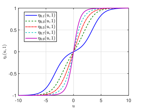
Figure 3: The threshold function $\eta_{\varepsilon}(u,v)$.

V-B Gaussian Distribution

The aim of this section is to explain how to obtain a closed-form expression for threshold functions targeting discrete Gaussian distributions. A discrete Gaussian distribution over $\mathbb{Z}$ with zero mean and width $\sigma_{g}$ is defined as

$$\rho_{\sigma_{g}}(z)=\frac{1}{S}e^{-z^{2}/\left(2\sigma_{g}^{2}\right)},$$

where $S=\sum_{k=-\infty}^{\infty}e^{-k^{2}/\left(2\sigma_{g}^{2}\right)}$. According to a tail bound on discrete Gaussian [40, Lem. 4.4], we have

$$\mathrm{Pr}_{z\sim\rho_{\sigma_{g}}(z)}\left(|z|>k\sigma_{g}\right)\leq 2e^{-k^{2}/2}$$

for any $k>0$. This implies that $\rho_{\sigma_{g}}(z)$ can be calculated from a finite range. E.g., we have $\mathrm{Pr}_{z\sim\rho_{\sigma_{g}}(z)}\left(|z|>10\sigma_{g}\right)\leq 3.86\times 10^{-22}$. If $\sigma_{g}=0.1$, then $\rho_{\sigma_{g}}(z)$ becomes equivalent to the ternary distribution with $\varepsilon\leq 0.5$.

Assume that we have observed $Y=u$ from model $Y=X+W$, with $X\sim p_{X}(x)=\rho_{\sigma_{g}}(x)$, $W\sim\mathrm{N}(0,v)$. Then the threshold functions are given by

$$\eta_{d}(u,v) =\frac{1}{S_{k}}\sum_{l=-k}^{k}le^{-\frac{l^{2}}{2\sigma_{g}^{2}}-\frac{\left(l-u\right)^{2}}{2v}},$$

$$\kappa_{d}(u,v) =\frac{1}{S_{k}}\sum_{l=-k}^{k}\left(l-\eta_{g}(u,v)\right)^{2}e^{-\frac{l^{2}}{2\sigma_{g}^{2}}-\frac{\left(l-u\right)^{2}}{2v}},$$

where $S_{k}=\sum_{l=-k}^{k}e^{-l^{2}/2\sigma_{g}^{2}-\left(l-u\right)^{2}/\left(2v\right)}$. Recall that we have mentioned evaluating $\eta_{d}(u,v)$ and $\kappa_{d}(u,v)$ is generally computationally intensive, and the fixed points of their state evolution equation are unfathomable. Fortunately, the sum of a discrete Gaussian and a continuous Gaussian resembles a continuous Gaussian if the discrete Gaussian is smooth [41, Lem. 9], so we can replace $\rho_{\sigma_{g}}(x)$ with $\mathrm{N}(x;0,\sigma_{g}^{2})$ with properly chosen $\sigma_{g}^{2}$. Let the signal distribution be $p_{X}(x)=\mathrm{N}(x;0,\sigma_{g}^{2})$, then it corresponds to another pair of threshold functions that have closed-forms:

$$\eta_{g}(u,v) =\frac{u\sigma_{g}^{2}}{\sigma_{g}^{2}+v},$$ (56)

$$\kappa_{g}(u,v) =\frac{v\sigma_{g}^{2}}{\sigma_{g}^{2}+v}.$$ (57)

The AMP algorithm using (56) (57) due to Gaussian distributions is referred to as AMPG.

V-C Parameters in Threshold Functions

In this section, we will inspect the effect of chosen parameters on the AMP algorithm, where the technique involved is about analyzing fixed points (see [42] for more backgrounds). First, the state evolution equation without the iteration subscript reads

$$\Psi(\widetilde{\tau}^{2})\triangleq\frac{1}{m}\sum_{j\in[n]}\sigma_{j}^{2}\mathbb{E}|\eta(X+\widetilde{\tau}/\sigma_{j}Z,\widetilde{\tau}^{2}/\sigma_{j}^{2})-X|^{2}+\sigma^{2}.$$ (58)

We refer to $\widetilde{\tau}^{2}$ as a fixed point of $\Psi(\widetilde{\tau}^{2})$ if $\Psi(\widetilde{\tau}^{2})=\widetilde{\tau}^{2}$. A fixed point is called stable if there exists $\epsilon\rightarrow 0^{+}$, such that $\Psi(\widetilde{\tau}^{2}+\epsilon)<\widetilde{\tau}^{2}$ and $\Psi(\widetilde{\tau}^{2}-\epsilon)>\widetilde{\tau}^{2}$. When $\Psi(0)=0$, the stability condition is relaxed to $\Psi(\widetilde{\tau}^{2}+\epsilon)<\widetilde{\tau}^{2}$. A fixed point is called unstable if it fails the stability condition. The estimation error of AMP is the smallest (resp. largest) if its $\Psi(\widetilde{\tau}^{2})$ converges to the lowest (resp. highest) stable fixed points [42].

For AMPT, we can demonstrate the impact of channel power $\left\{\sigma_{j}^{2}\right\}$ and sparsity $\left(1-\varepsilon\right)$ through the following proposition. Its proof is shown in Appendix E.

Proposition 1.

There exists a minimum $\epsilon^{\prime}>0$, such that $\forall\sigma^{2}>\epsilon^{\prime}$, the highest stable fixed point of Eq. (71) is $\Psi(\varepsilon/m\sum_{j\in[n]}\sigma_{j}^{2}+\sigma^{2})=\varepsilon/m\sum_{j\in[n]}\sigma_{j}^{2}+\sigma^{2}$.

In the proposition, the highest fixed point is unique if $\partial\Psi(\widetilde{\tau}^{2})/\partial\widetilde{\tau}^{2}<1$ $\forall\widetilde{\tau}^{2}>0$, which means the increment of $\Psi(\widetilde{\tau}^{2})$ is never larger than that of $f(\widetilde{\tau}^{2})=\widetilde{\tau}^{2}$. One implication of the proposition is, a stronger lattice reduction method can help to make the fixed point smaller. E.g., with b-KZ, one has

$$\sum_{j\in[n]}\sigma_{j}^{2}\leq\sum_{j\in[n]}\frac{\sqrt{j+3}}{2}\lambda_{j}(\mathbf{H})$$

for $n\geq 2$. Another implication is, the performance of AMP should be better if the real spark $\varepsilon$ is small. There is however no genie granting which $\varepsilon$ fits the actual a priori knowledge. According to our simulations, $\varepsilon=0.5$ is a good trade-off.

For AMPG, similar analysis on fixed points can reveal the impact of $\left\{\sigma_{j}^{2}\right\}$ and prior variance $\sigma_{g}^{2}$. By substituting Eq. (56) to (58), the fixed point function becomes

$$\Psi(\widetilde{\tau}^{2})=\sigma^{2}+\frac{1}{m}\sum_{j\in[n]}\frac{\widetilde{\tau}^{2}\sigma_{j}^{2}\sigma_{g}^{2}}{\widetilde{\tau}^{2}+\sigma_{j}^{2}\sigma_{g}^{2}}.$$ (59)

Let $\sigma_{\min}^{2}\triangleq\min_{j}\sigma_{j}^{2}$ and $\sigma_{\max}^{2}\triangleq\max_{j}\sigma_{j}^{2}$, we have

$$\frac{n\widetilde{\tau}^{2}\sigma_{\min}^{2}\sigma_{g}^{2}}{m\left(\widetilde{\tau}^{2}+\sigma_{\min}^{2}\sigma_{g}^{2}\right)}\leq\Psi(\widetilde{\tau}^{2})-\sigma^{2}\leq\frac{n\widetilde{\tau}^{2}\sigma_{\max}^{2}\sigma_{g}^{2}}{m\left(\widetilde{\tau}^{2}+\sigma_{\max}^{2}\sigma_{g}^{2}\right)}.$$

As a consequence, one can easily prove that Eq. (59) has a unique stable fixed point that satisfies $\widetilde{\tau}^{2}\in[\widetilde{\tau}_{\min}^{2},\widetilde{\tau}_{\max}^{2}]$, where

$$\widetilde{\tau}_{\min}^{2} =\frac{1}{2}\left(\sigma^{2}+\left(\frac{n}{m}-1\right)\sigma_{\min}^{2}\sigma_{g}^{2}\right)$$

$$+\frac{1}{2}\sqrt{\left(\sigma^{2}+\left(\frac{n}{m}-1\right)\sigma_{\min}^{2}\sigma_{g}^{2}\right)^{2}+4\sigma^{2}\sigma_{\min}^{2}\sigma_{g}^{2}},$$ (60)

and $\widetilde{\tau}_{\max}^{2}$ is defined by replacing $\sigma_{\min}^{2}$ with $\sigma_{\max}^{2}$ in (60). In order to make the fixed point small, one should also make the lattice basis short. The setting of $\sigma_{g}^{2}$ is also a trade-off: it should be set smaller to yield a lower fixed point, but there should be a minimum for it so that the imposed signal distribution still reflects discrete Gaussian information. A general principle for finding the trade-off value is left as an open question.

V-D Complexity of AMP

The complexity is assessed by counting the number of floating-point operations (flops). For the threshold functions (54) (55) of AMPT, we can use $\sinh\left(\frac{u}{v}\right)\approx\frac{u}{v},$ $\cosh\left(\frac{u}{v}\right)\approx 1+\frac{u^{2}}{2v^{2}}$ for small $u/v$ since $\sinh x=\sum_{k=0}^{\infty}\frac{x^{2k}}{\left(2k\right)!}$, $\cosh x=\sum_{k=0}^{\infty}\frac{x^{2k+1}}{\left(2k+1\right)!}$. Outer bounding (54) (55) is also possible for large $u/v$, so we can approximate (54) (55) by $O(1)$ flops. The $O(1)$ complexity also holds for (56) (57) of AMPG. In conclusion, the complexity of our AMP algorithm is $O(mnT)$. On the contrary, a full enumeration with a ternary constraint already requires at least $O(3^{n})$ flops, and ZF/SIC requires $O(mn^{2})$ flops.

VI Simulations

In this section, the symbol error rate (SER) and complexity performance of the proposed hybrid precoding scheme are examined through Monte Carlo simulations. The impacts of chosen parameters in the threshold functions are also studied. For comparison, the sphere precoding method [1, 2] and LR aided precoding methods based on ZF/SIC are also tested. Throughout this section, b-LLL with list size $1$ is adopted as the default LR option, and we refer to [15] for a full comparison of different reduction algorithms. In all the AMP algorithms, we set $\sigma^{2}=\left\|\mathbf{y}-\mathbf{H}\hat{\mathbf{x}}\right\|^{2}/m^{1.5}$ (so as to approximate $\left\|\mathbf{y}-\mathbf{H}\mathbf{x}^{\mathrm{cvp}}\right\|^{2}/m$), and $T=20$.

First, Fig. 4 illustrates the SNR versus SER performance of different algorithms using a modulation size $M=32$ for antenna configurations $m=n=8$ and $m=n=14$. We set $\varepsilon=0.5$ in AMPT and $\sigma_{g}^{2}=2$ in AMPG. As shown in the figure, both AMPT and AMPG can improve the performance of LR-ZF/SIC towards that of sphere precoding. These gains become more evident as the size of the system grows from $m=n=8$ to $m=n=14$, in which AMPT improves LR-ZF by $3$dB and LR-SIC by $0.8$dB.

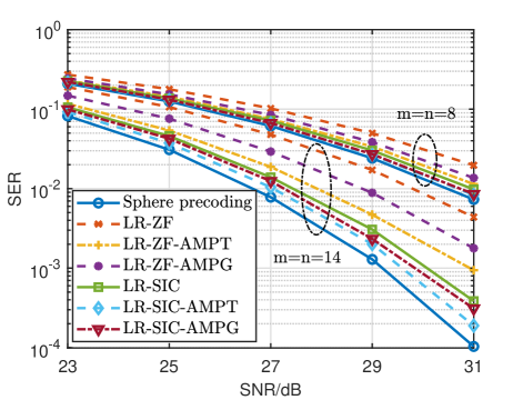
Figure 4: The symbol error rate of different algorithms.

Next, we examine the effect of choosing different spark values in AMPT, with $M=32,64$ and $m=n=14$. The AMPT algorithm using the real spark (by comparing to sphere precoding) to noted as AMPT-$\varepsilon^{\prime}$. Two other references are $\varepsilon=0.5$ and $\varepsilon=1$. According to Fig. 5, the idealised AMPT-$\varepsilon^{\prime}$ performs $1$dB better than AMPT-$1$, but is within $0.2$dB distance to AMPT-$.5$. This suggests that in practice we can adopt $\varepsilon=0.5$ as a reasonable configuration.

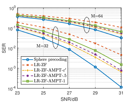
Figure 5: The impact of spark values in AMPT with $m=n=14$.

Similarly, the effect of chosen variance $\sigma_{g}^{2}$ in AMPG is studied in Fig. 6. The suffixes after AMPG refer to setting $\sigma_{g}^{2}$ as $\sigma_{g^{\prime}}^{2}=\left\|\mathbf{x}^{\mathrm{cvp}}-\hat{\mathbf{x}}\right\|^{2}/n$, and $2$, $20$, $200$, respectively. Other configurations are identical to those in Fig. 5. An observation from Fig. 6 is that the AMPG-$\sigma_{g^{\prime}}^{2}$ algorithm is not better than those with manually chosen variances; this refeclts the fact that $\sigma_{g}^{2}$ can not be too small so as to reflect discrete Gaussian information (c.f. Section V-C). In addition, the trade-offs $\sigma_{g}^{2}=2,20$ work better than the too large value $\sigma_{g}^{2}=200$ and the too small value ($\sigma_{g}^{2}=\sigma_{g^{\prime}}^{2}$).

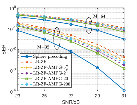
Figure 6: The impact of variance $\sigma_{g}^{2}$ in AMPG with $m=n=14$.

In the last example, we examine the complexity of our AMP algorithms. We use estimations in Section V-D to measure the complexity of ZF/SIC and AMP. As for the sphere decoding algorithm, it is implemented after b-LLL so as to decrease its complexity. All algorithms can take the benefits of b-LLL, and the complexity costed by lattice reduction is not counted for all of them. The actual complexity of sphere precoding depends on the inputs, so we count the number of nodes it visited, and assign $2k+7$ flops to a visited node in layer $k$ [15]. From Fig. 7, we can see that AMP with a constant iteration number, e.g., $T=10$ or $T=20$, is adding little complexity budget to that of ZF/SIC. On the contrary, the exponential complexity of sphere decoding makes it at least $200$ times more complicated than our ZF/SIC+AMP scheme in dimension $n=22$.

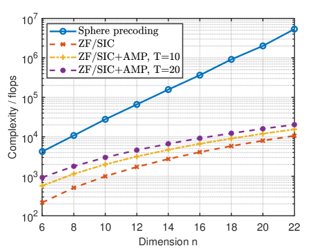
Figure 7: The complexity of different algorithms.

VII Extension to Data Detection in Massive MIMO

The developed hybrid precoding (decoding) scheme for VP can be directly extended to address the data detection problem in small-scaled MIMO systems whose underlying CVP has more constraints. We omit the presentation of similar results. The more interesting extension that we will pursuit in this section is to data detection in massive MIMO systems, where the base stations are equipped with hundreds of antennas to simultaneously serve tens of users [43]. In the classical i.i.d. frequency-flat Rayleigh fading MIMO channels, the set-up of massive MIMO implies that channel matrix is extremely tall in the corresponding CVP. As a result, we can regard these lattice bases (channel matrices) that are short and orthogonal as naturally reduced. This suggests we can apply our hybrid scheme to massive MIMO without using lattice reduction.

VII-A System Model and the Reduced Basis

With a slight abuse of notation, we write the system model in the uplink of massive MIMO as

$$\mathbf{y}=\mathbf{H}\mathbf{x}+\mathbf{w},$$ (61)

where $\mathbf{y}\in\mathbb{R}^{m}$ is the received signal vector at the base station, $\mathbf{H}\in\mathbb{R}^{m\times n}$ denotes the channel matrix whose entries follow the distribution of $\mathrm{N}(0,1)$, $\mathbf{w}\in\mathbb{R}^{m}$ is the additive noise vector whose entries admit $\mathrm{N}(0,\sigma^{2})$, and $\mathbf{x}\in\mathcal{M}^{n}$ is the transmitted signal vector that contains the data symbols from all the user terminals. For ease of presentation, we set the constellation as $\mathcal{M}=\{-M,-M+1,\ldots,M-1,M\}$. The special constraint in massive MIMO is that $m\gg n$, based on which the simple LMMSE detection suffices to provide near-optimal performance. Let $\sigma_{s}^{2}$ denote the averaged power of $\mathbf{x}$, by using LMMSE equalization we have

$$\mathbf{x}^{\mathrm{lmmse}}=\lfloor\left(\mathbf{H}^{\top}\mathbf{H}+\sigma^{2}/\sigma_{s}^{2}\mathbf{I}_{n}\right)^{-1}\mathbf{H}^{\top}\mathbf{y}\rceil.$$

It is well known that LMMSE is a variant of ZF and they become equivalent as $\sigma^{2}\rightarrow 0$, and its computational complexity is $O\left(n^{3}+mn^{2}\right)$.

TABLE II: The values $\hat{x}_{i}-x_{i}^{\mathrm{cvp}}$ with $i\in[n]$ and their probabilities in data detection.

error	distance	$-4$	$-3$	$-2$	$-1$	$0$	$1$	$2$	$3$	$4$
$m=16,n=8$	ZF	$0$	$0$	$0.0003$	$0.0796$	$0.8458$	$0.0744$	$0$	$0$	$0$
$\mathrm{SNR}=10\mathrm{dB}$	LR-ZF	$0$	$0$	$0.0021$	$0.0825$	$0.8285$	$0.0854$	$0.0015$	$0$	$0$
$m=8,n=8$	ZF	$0.0090$	$0.0174$	$0.0401$	$0.1594$	$0.5035$	$0.1544$	$0.0409$	$0.0163$	$0.0077$
$\mathrm{SNR}=10\mathrm{dB}$	LR-ZF	$0.0086$	$0.0166$	$0.0369$	$0.1090$	$0.6105$	$0.1087$	$0.0334$	$0.0160$	$0.0103$
$m=16,n=8$	ZF	$0$	$0$	$0$	$0.0003$	$0.9995$	$0.0002$	$0$	$0$	$0$
$\mathrm{SNR}=30\mathrm{dB}$	LR-ZF	$0$	$0$	$0$	$0.0001$	$0.9999$	$0$	$0$	$0$	$0$
$m=8,n=8$	ZF	$0.0057$	$0.0077$	$0.0195$	$0.1074$	$0.6937$	$0.1046$	$0.0176$	$0.0079$	$0.0043$
$\mathrm{SNR}=30\mathrm{dB}$	LR-ZF	$0.0018$	$0.0027$	$0.0037$	$0.0181$	$0.9299$	$0.0170$	$0.0056$	$0.0032$	$0.0022$

Here, we notice that channel matrices in massive MIMO represent extremely good lattice bases. For instance, a tall channel matrix with dimension $2n\times n$ already represents a lattice basis that often outcompetes boosted KZ (to our knowledge, this is almost the strongest lattice reduction). To support this argument, we show the symbol-wise error distance in decoding (61) by using LR (boosted KZ) aided ZF and ZF. Table II reveals this result using $M=14$, $\left(m,n\right)=\left(16,8\right)$, $\left(m,n\right)=(8,8)$, $\mathrm{SNR}=10\mathrm{dB}$ and $\mathrm{SNR}=30\mathrm{dB}$. We have the following observations from the table: For a square channel matrix with $m=n$, LR-ZF indeed has smaller error ratios than those of ZF. But as the channel matrix becomes tall with $m=2n$, ZF performs close to LR-ZF ($\mathrm{SNR}=30\mathrm{dB}$) or even outperforms LR-ZF ($\mathrm{SNR}=10\mathrm{dB}$). Similar observations can also be made for other sizes of constellations, SNRs and sizes of the system.

This phenomenon is however not a surprise: as $m/n$ grows larger, the vectors $\mathbf{h}_{1},\ldots,\mathbf{h}_{n}$ in the basis become almost mutually orthogonal. Since any linear combination of these vectors can only be longer, $\mathbf{h}_{1},\ldots,\mathbf{h}_{n}$ would become the shortest $n$ independent vectors of $\mathcal{L}(\mathbf{H})$ and we have $\left\|\mathbf{h}_{i}\right\|=\lambda_{i}(\mathbf{H})$ for $i\in[n]$. Compared to boosted KZ which only upper bounds $\left\|\mathbf{h}_{i}\right\|$ to $O(\sqrt{i})\lambda_{i}(\mathbf{H})$, these shortest independent vectors are much more desirable.

VII-B Simulations

To see the advantage of using hybrid decoding in massive MIMO, we run simulations to obtain SERs for different algorithms. With a relatively large constellation size, the AMP algorithm using exact a priori knowledge no longer suits our problem as it is slow, unstable and divergent [22, 23]. It is therefore reasonable to adopt AMPG [20, 26, 25] as a benchmark, because it has the best convergence behavior among all AMP-based algorithms without using hybrid decoding. Another benchmark is the LMMSE estimator, and we will use AMPG or AMPT (both have complexity $O(mnT)$) as the algorithm in “Phase 2” based on it.

The SERs of these algorithms are shown in Figs. 8 and 9, with constellation size $M=14,22$ and system dimension $(m,n)=(128,48),(128,64)$. As revealed in the figures, both AMPG and AMPT can improve the performance of LMMSE to a certain degree, but the improvement of AMPT is more evident as its threshold functions are non-linear. Note that the hybrid scheme can also employ AMPG as the first-round algorithm to make the total complexity of hybrid decoding as $O(mnT)$, but the bad performance of AMPG at high SNR dictates the overall performance.

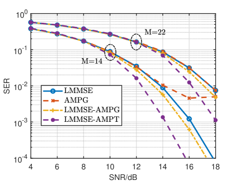
Figure 8: The symbol error rate of different algorithms with $m=128$, $n=48$.

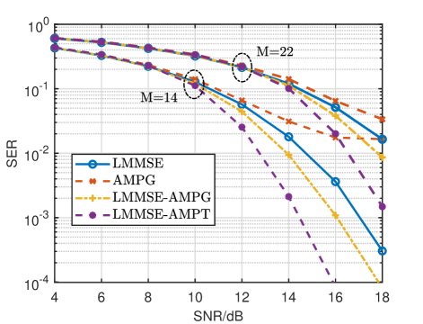
Figure 9: The symbol error rate of different algorithms with $m=128$, $n=64$.

VIII Conclusions

In this work, we have presented a hybrid precoding scheme for VP. The precoding problem in VP is about solving CVP in a lattice, and this problem is quite general because the signal space lies in integers $\mathbb{Z}$. After performing LR aided ZF/SIC, we indicated that the signal space had been significantly reduced, and this information paved the way for the application of the celebrated AMP algorithm. Considering ternary distributions and Gaussian distributions, we have designed threshold functions that have closed-form expressions. Our simulations showed that attaching AMP to LR-ZF or LR-SIC can provide around $0.5$dB to $2.5$dB gain in SER for VP, where the AMP algorithm only incurred complexity in the order of $O(mnT)$. Lastly, we have also demonstrated that the hybrid scheme can be extended to data detection in massive MIMO without using lattice reduction.

Appendix A On using reduced bases for AMP

In our precoding problem, the mixing matrix $\mathbf{H}$ comes from lattice reduction rather than naturally having i.i.d. Gaussian entries. Although $\mathbf{H}$ is known to be short and nearly orthogonal after lattice reduction, its statistical information cannot be exactly analyzed by only using the theory of lattices. To provide some complements to our simulation results that have confirmed the feasibility of using reduced bases for AMP, our aim in this section is to explain why the reduce bases can work in principle.

The first reason is that all the edges on the bipartite graph are weak for a reduced basis. It was suggested by Rangan et al. [35] that the AMP-style approximations are effective if the messages are propagating on weak edges. In their definition [35, P. 4578], the entries of a mixing matrix $\mathbf{H}$ are called “small” if no individual component can have a significant effect on the row-sum or column-sum of $\mathbf{H}$. Here we define a “small” factor to measure this effect:

$$\mu_{s}\left(\mathbf{H}\right)\triangleq\max_{i\in[m],j\in[n]}\left(\max\left(\frac{|H_{i,j}|}{\sum_{i}|H_{i,j}|},\frac{|H_{i,j}|}{\sum_{j}|H_{i,j}|}\right)\right).$$

In Fig. 10, we plot the averaged “small” factors $\mathbb{E}\mu_{s}\left(\mathbf{H}\right)$ produced by different methods. The lattice reduction methods, noted as “LLL”, “b-LLL”, “KZ” and “b-KZ” , are applied on the inverse of Gaussian random matrices of rank $n$. The “small” factors of Gaussian random matrices with $\mathrm{N}(0,1)$ entries, noted as “Gaussian”, and those before lattice reduction, noted as “Before LR”, are also included for comparison. One thing we can observe from the figure is that the lattice reduction methods behave as good as Gaussian entries. We also note the figure shows the bases before lattice reduction already exhibit rather weak edges, but this does not suggest they correspond to more efficient AMP methods. We notice that a small $\mu_{s}\left(\mathbf{H}\right)$ is only a necessary condition for AMP. Specifically, for a matrix with $H_{i,j}=1,\thinspace\forall i,j$, we have $\mu_{s}\left(\mathbf{H}\right)=1/n$ that is arbitrarily small while $\mathbf{H}$ is ill-conditioned.

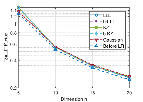
Figure 10: The averaged “small” factors of different algorithms for $\mathbf{H}\in\mathbb{R}^{n\times n}$.

The second reason is that a reduced basis has a small coherence parameter [44] defined by

$$\mu_{c}\left(\mathbf{H}\right)\triangleq\max_{1\leq i\neq j\leq n}|\mathbf{h}_{i}^{\top}\mathbf{h}_{j}|/\left\|\mathbf{h}_{i}\right\|\left\|\mathbf{h}_{j}\right\|,$$

where $\mathbf{H}=\left[\mathbf{h}_{1},\ldots\thinspace,\mathbf{h}_{n}\right]$. This metric can reflect the column-wise independence. In Fig. 11, we plot the expected coherence parameter $\mathbb{E}\mu_{c}\left(\mathbf{H}\right)$ of different lattice reduction algorithms from dimensions $5$ to $20$, and include Gaussian bases and the bases before LR for comparison. Other settings are the same as those in Fig. 10. As shown in Fig. 11, the coherence parameters can be significantly reduced after using lattice reduction. Most importantly, Fig. 11 suggests that a coherence parameter of $\mu_{c}\left(\mathbf{H}\right)=0.5$ that corresponds to a Gaussian random matrix of dimension $n=40$ is equivalent to those of lattice reduction with much smaller dimensions, e.g., $n=15$ with LLL and $n=20$ with boosted LLL.

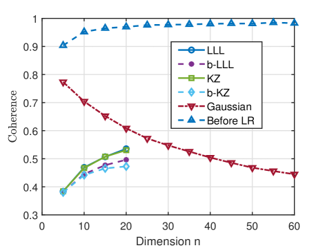
Figure 11: The coherence parameters of different algorithms for $\mathbf{H}\in\mathbb{R}^{n\times n}$.

Appendix B Proof of Eq. (14) in Theorem 1

When proving the energy efficiency of b-KZ aided SIC/ZF, the following lemma would be needed. Remind that $\mathbf{H}=\mathbf{QR}$ is the QR factorization.

Lemma 2 ([15]).

Suppose a basis $\mathbf{H}$ is b-KZ reduced, then this basis conforms to

$$\lambda_{1}(\mathbf{H})^{2}\leq\frac{8i}{9}(i-1)^{\ln(i-1)/2}R_{i,i}^{2},$$ (62)

$$\left\|\mathbf{h}_{i}\right\|^{2}\leq\Big{(}1+\frac{2i}{9}(i-1)^{1+\ln(i-1)/2}\Big{)}R_{i,i}^{2}$$ (63)

for $1\leq i\leq n$, and

$$R_{k-j+1,k-j+1}^{2}\leq\frac{8j}{9}(j-1)^{\ln(j-1)/2}R_{k,k}^{2}$$ (64)

for $2\leq k\leq n$, $j\leq k$.

Under the unitary transform $\mathbf{Q}^{\top}$, we aim to prove an equivalence of (12) as

$$\left\|\mathbf{\bar{y}}-\mathbf{R}\hat{\mathbf{x}}\right\|\leq\eta_{n}\min_{\mathbf{x}\in\mathbb{Z}^{n}}\left\|\mathbf{\bar{\mathbf{y}}}-\mathbf{Rx}\right\|,$$ (65)

with $\mathbf{\mathbf{\bar{y}}}=\mathbf{Q}^{\top}\mathbf{y}$. Let $\mathbf{v}^{\mathrm{cvp}}=\mathbf{R}\mathbf{x}^{\mathrm{cvp}}$ be the closest vector to $\mathbf{\mathbf{\bar{y}}}$, and $\mathbf{v}^{\mathrm{sic}}=\mathbf{R}\mathbf{x}^{\mathrm{sic}}$ be the vector founded by SIC. As the SIC parallelepiped generally mismatches the Voronoi region, we need to investigate the relation of $x_{n}^{\mathrm{cvp}}$ and $x_{n}^{\mathrm{sic}}=\lfloor\bar{y}_{n}/R_{n,n}\rceil$ as in that in [33]. If $x_{n}^{\mathrm{cvp}}=x_{n}^{\mathrm{sic}}$, we only need to investigate $\eta_{n-1}$ in another $n-1$ dimensional CVP by setting $\mathbf{\bar{y}}\leftarrow\mathbf{\bar{y}}-\mathbf{r}_{n}x_{n}^{\mathrm{sic}}$: $\left\|\mathbf{\bar{y}}-\mathbf{R}_{1:n,1:n-1}\mathbf{x}_{1:n-1}^{\mathrm{sic}}\right\|\leq\eta_{n-1}\min_{\mathbf{x}\in\mathbb{Z}^{n-1}}\left\|\mathbf{\bar{y}}-\mathbf{R}_{1:n,1:n-1}\mathbf{x}\right\|$. When this situation continues till the first layer, one clearly has $\eta_{1}=1$. Generally, we can assume that this mismatch first happens in the $k$th layer, i.e., assume $x_{k}^{\mathrm{cvp}}\neq x_{k}^{\mathrm{sic}},$ $k\in\{2,\ldots\thinspace,n\}$, then $|\bar{y}_{k}/R_{k,k}-x_{k}^{\mathrm{cvp}}|\geq\frac{1}{2}$, and

$$\left\|\bar{\mathbf{y}}-\mathbf{v}^{\mathrm{cvp}}\right\|^{2}\geq r_{k,k}^{2}(\bar{y}_{k}/R_{k,k}-x_{k}^{\mathrm{cvp}})^{2}\geq R_{k,k}^{2}/4.$$ (66)

According to (64) of b-KZ, we have $R_{k-j+1,k-j+1}^{2}\leq\frac{8j}{9}(j-1)^{\ln(j-1)/2}R_{k,k}^{2}$, then the SIC solution $\mathbf{R}_{1:n,1:k}\mathbf{x}_{1:k}^{\mathrm{sic}}$ satisfies

$$\left\|\bar{\mathbf{y}}-\mathbf{R}_{1:n,1:k}\mathbf{x}_{1:k}^{\mathrm{sic}}\right\|^{2} \leq\frac{1}{4}\sum_{i=1}^{k}R_{i,i}^{2}$$

$$\leq\left(\frac{1}{4}+\frac{2k}{9}\left(k-1\right)^{1+\ln(k-1)/2}\right)R_{k,k}^{2}.$$ (67)

Combining (67) and (66), and choose $k=n$ in the worst case, we have

$$\left\|\bar{\mathbf{y}}-\mathbf{v}^{\mathrm{sic}}\right\|^{2}\leq\left(1+\frac{8n}{9}\left(n-1\right)^{1+\ln(n-1)/2}\right)\left\|\bar{\mathbf{y}}-\mathbf{v}^{\mathrm{cvp}}\right\|^{2}.$$

Appendix C Proof of Theorem 2

The energy efficiency of b-LLL/b-KZ aided ZF precoding is non-trivial to prove because we cannot employ the size reduction conditions to claim an upper bound for $(\mathbf{A}^{i})_{1,1}^{-1}$ as that in [32, Eq. (65)], in which $\mathbf{A}^{i}=\mathbf{R}_{i:n,i:n}^{\top}\mathbf{R}_{i:n,i:n}$. This condition is crucial as one already has

$$\sin^{2}\theta_{i}=\frac{1}{\left\|\mathbf{h}_{i}\right\|^{2}(\mathbf{A}^{i})_{1,1}^{-1}}$$

according to [32, Appx. I], where $\theta_{i}$ is the angle between $\mathbf{h}_{i}$ and $\mathrm{span}(\mathbf{h}_{1},\ldots,\thinspace\mathbf{h}_{i-1},\mathbf{h}_{i+1},\ldots,\thinspace\mathbf{h}_{n})$. The following lemma proves a lower bound for $\sin^{2}\theta_{i}$ by only invoking the relation between $\left\|\mathbf{h}_{i}\right\|^{2}$ and $R_{i,i}^{2}$.

Lemma 3.

Let $\mathbf{H}$ be a b-KZ reduced basis, then it satisfies $\sin^{2}\theta_{i}\geq\left(\prod_{k=i}^{n}k^{2+\ln(k)/2}\right)^{-1}.$

Proof:

Define $\mathbf{M}^{k}=\mathbf{R}_{i:k,i:k}^{-1}$ along with $\mathbf{M}^{i}=R_{i,i}^{-1}$, then

$$\mathbf{M}^{k}=\left[\begin{array}[]{cc}\mathbf{M}^{k-1}&R_{k,k}^{-1}\mathbf{M}^{k-1}\mathbf{R}_{i:k-1,k}\\ \mathbf{0}&R_{k,k}^{-1}\end{array}\right].$$

By using Cauchy–Schwarz inequality on $\mathbf{M}_{1,:}^{k-1}\mathbf{R}_{i:k-1,k}$, we also have

$$\left\|\mathbf{M}_{1,:}^{k}\right\|^{2} =\left\|\mathbf{M}_{1,:}^{k-1}\right\|^{2}+\left(R_{k,k}^{-1}\mathbf{M}_{1,:}^{k-1}\mathbf{R}_{i:k-1,k}\right)^{2}$$

$$\leq\left\|\mathbf{M}_{1,:}^{k-1}\right\|^{2}\left(1+R_{k,k}^{-2}\left\|\mathbf{R}_{i:k-1,k}\right\|^{2}\right).$$ (68)

It is evident that $\left\|\mathbf{R}_{i:k-1,k}\right\|^{2}\leq\left\|\mathbf{h}_{k}\right\|^{2}-R_{k,k}^{2}\overset{(a)}{\leq}\Big{(}1+\frac{2k}{9}(k-1)^{1+\ln(k-1)/2}\Big{)}R_{k,k}^{2}-R_{k,k}^{2}$, where (a) is due to inequality (63), so that $R_{k,k}^{-2}\left\|\mathbf{R}_{i:k-1,k}\right\|^{2}\leq\frac{2k}{9}(k-1)^{1+\ln(k-1)/2}$. Substitute this into (68), then

$$\left\|\mathbf{M}_{1,:}^{k}\right\|^{2} \leq\left\|\mathbf{M}_{1,:}^{k-1}\right\|^{2}\left(1+\frac{2k}{9}(k-1)^{1+\ln(k-1)/2}\right)$$

$$\leq\left\|\mathbf{M}_{1,:}^{k-1}\right\|^{2}k^{2+\ln(k)/2}.$$

By induction, one has

$$(\mathbf{A}^{i})_{1,1}^{-1}=\left\|\mathbf{M}_{1,:}^{n}\right\|^{2}\leq R_{i,i}^{-2}\prod_{k=i+1}^{n}k^{2+\ln(k)/2}.$$

and thus

$$\sin^{2}\theta_{i}\geq\frac{R_{i,i}^{2}}{\left\|\mathbf{h}_{i}\right\|^{2}\prod_{k=i+1}^{n}k^{2+\ln(k)/2}}\geq\left(\prod_{k=i}^{n}k^{2+\ln(k)/2}\right)^{-1},$$

where the second inequality is due to Lem. 2. ∎

With the same technique as above, we can bound $\sin^{2}\theta_{i}$ for b-LLL.

Lemma 4.

Let $\mathbf{H}$ be a b-LLL reduced basis, then it satisfies $\sin^{2}\theta_{i}\geq\left(\prod_{k=i}^{n}\beta^{k-1}\right)^{-1}$.

We proceed to investigate inequality (65). Let $\mathbf{v}^{\mathrm{cvp}}=\mathbf{R}\mathbf{x}^{\mathrm{cvp}}$ be the closest vector to $\mathbf{\mathbf{\bar{y}}}$, and $\mathbf{v}^{\mathrm{zf}}=\mathbf{R}\mathbf{x}^{\mathrm{zf}}$ be the vector found by ZF. Define $\mathbf{v}^{\mathrm{cvp}}-\mathbf{v}^{\mathrm{zf}}=\sum_{i=1}^{n}\phi_{i}\mathbf{h}_{i}$ with $\phi_{i}\in\mathbb{Z}$. If $\mathbf{v}^{\mathrm{cvp}}=\mathbf{v}^{\mathrm{zf}}$, then the energy efficiency $\eta_{n}=1$. If $\mathbf{v}^{\mathrm{cvp}}\neq\mathbf{v}^{\mathrm{zf}},$ then

$$\left\|\mathbf{v}^{\mathrm{cvp}}-\mathbf{v}^{\mathrm{zf}}\right\|\leq\sum_{j=1}^{n}\left\|\phi_{j}\mathbf{h}_{j}\right\|.$$

At the same time, we have

$$\mathbf{v}^{\mathrm{cvp}}-\bar{\mathbf{y}} =\mathbf{v}^{\mathrm{cvp}}-\mathbf{v}^{\mathrm{zf}}+\mathbf{v}^{\mathrm{zf}}-\bar{\mathbf{y}}$$

$$=(\phi_{k}+\phi_{k}^{\mathrm{zf}})\mathbf{h}_{k}+\mathbf{m}^{\prime},$$

where $\mathbf{m}^{\prime}\in\mathrm{span}(\mathbf{h}_{1},\ldots,\thinspace\mathbf{h}_{k-1},\mathbf{h}_{k+1},\ldots,\thinspace\mathbf{h}_{n})$, $\mathbf{v}^{\mathrm{zf}}-\bar{\mathbf{y}}=\sum_{i=1}^{n}\phi_{i}^{\mathrm{zf}}\mathbf{h}_{i}$ satisfies $|\phi_{i}^{\mathrm{zf}}|\leq 1/2$ $\forall i$, and $k\triangleq\arg\max_{i}\left\|\phi_{i}\mathbf{h}_{i}\right\|$. From Lem. 3, $\left\|(\phi_{k}+\phi_{k}^{\mathrm{zf}})\mathbf{h}_{k}+\mathbf{m}^{\prime}\right\|\geq|\phi_{k}+\phi_{k}^{\mathrm{zf}}|\left(\prod_{j=k}^{n}j^{2+\ln(j)/2}\right)^{-1}\left\|\mathbf{h}_{k}\right\|$, so that

$$\left\|\mathbf{v}^{\mathrm{cvp}}-\bar{\mathbf{y}}\right\|\geq|\phi_{k}|\left(2\prod_{j=k}^{n}j^{2+\ln(j)/2}\right)^{-1}\left\|\mathbf{h}_{k}\right\|$$

as $|\phi_{k}+\phi_{k}^{\mathrm{zf}}|\geq|\phi_{k}|/2$. According to the triangle inequality, one has for b-KZ that

$$\left\|\mathbf{v}^{\mathrm{zf}}-\bar{\mathbf{y}}\right\| \leq\left\|\mathbf{v}^{\mathrm{zf}}-\mathbf{v}^{\mathrm{cvp}}\right\|+\left\|\mathbf{v}^{\mathrm{cvp}}-\bar{\mathbf{y}}\right\|$$

$$\leq\left(2n\prod_{j=1}^{n}j^{2+\ln(j)/2}+1\right)\left\|\mathbf{v}^{\mathrm{cvp}}-\bar{\mathbf{y}}\right\|.$$

One can similarly prove for b-LLL that

$$\left\|\mathbf{v}^{\mathrm{zf}}-\bar{\mathbf{y}}\right\|\leq\left(2n\prod_{j=1}^{n}\beta^{j-1}+1\right)\left\|\mathbf{v}^{\mathrm{cvp}}-\bar{\mathbf{y}}\right\|.$$

Appendix D Proof of Theorem 3

Proof:

We follow [20, Sec. 1.3] to analysis the state evolution equation (52). Let the observation equation be $\mathbf{y}^{t}=\mathbf{H}^{t}\bar{\mathbf{x}}+\mathbf{w}$, where the distribution of $\bar{\mathbf{x}}$ is denoted by $p_{X}$, $H_{b,i}\sim\mathrm{N}(0,\sigma_{i}^{2}/m)$, and $w_{i}\in\mathrm{N}(0,\sigma^{2})$. Without the Onsager term, the residual equation becomes:

$$\mathbf{r}^{t}=\mathbf{y}^{t}-\mathbf{H}^{t}\mathbf{x}^{t}.$$ (69)

Along with with independently generated $\left\{\mathbf{H}^{t}\right\}$, the estimation equation becomes:

$$\mathbf{x}^{t+1}=\eta(\Theta\mathbf{H}^{t\top}\mathbf{r}^{t}+\mathbf{x}^{t},\Theta\tau_{t}^{2}\mathbf{1}).$$ (70)

Then we evaluate the first input for the threshold function $\eta$: $\Theta\mathbf{H}^{t\top}\mathbf{r}^{t}+\mathbf{x}^{t}=$

$$\Theta\mathbf{H}^{t\top}(\mathbf{H}^{t}\bar{\mathbf{x}}+\mathbf{w}-\mathbf{H}^{t}\mathbf{x}^{t})+\mathbf{x}^{t}$$

$$= \bar{\mathbf{x}}+\underset{\triangleq\mathbf{u}}{\underbrace{(\Theta\mathbf{H}^{t\top}\mathbf{H}^{t}-\mathbf{I})(\bar{\mathbf{x}}-\mathbf{x}^{t})}}+\underset{\triangleq\mathbf{v}}{\underbrace{\Theta\mathbf{H}^{t\top}\mathbf{w}}.}$$

Regarding term $\mathbf{v}$, it satisfies $\mathbb{V}(v_{i})=\frac{\sigma_{i}^{2}}{m}\times\frac{1}{\sigma_{i}^{4}}\times m\times\sigma^{2}$, which means $v_{i}\sim\mathrm{N}(0,\sigma^{2}/\sigma_{i}^{2})$. As for the statistics of term $\bm{u}$, we need the following basic algebra to measure term $\Theta\mathbf{H}^{t\top}\mathbf{H}^{t}-\mathbf{I}$:

Suppose that we have two independent Gaussian columns $\mathbf{h}_{i}$ and $\mathbf{h}_{j}$ whose entries are generated from $\mathrm{N}(c,\sigma_{i}^{2}/m)$ and $\mathrm{N}(c,\sigma_{j}^{2}/m)$ respectively. Then $\forall i\neq j$, we have $\mathbb{E}(\mathbf{h}_{i}^{\top}\mathbf{h}_{j})=mc^{2}$ and $\mathbb{V}(\mathbf{h}_{i}^{\top}\mathbf{h}_{j})=\sigma_{i}^{2}\sigma_{j}^{2}/m+c^{2}(\sigma_{i}^{2}+\sigma_{j}^{2})$. For $i=j$, we have $\mathbb{E}(\left\|\mathbf{h}_{i}\right\|^{2})=mc^{2}+\sigma_{i}^{2}$ and $\mathbb{V}(\left\|\mathbf{h}_{i}\right\|^{2})=2\sigma_{i}^{4}/m^{2}+4c^{2}\sigma_{i}^{2}/m$.

Further denote the covariance matrix of $\bar{\mathbf{x}}-\mathbf{x}^{t}$ as $\mathrm{diag}(\hat{\tau}_{t,1}^{2},...\thinspace,\hat{\tau}_{t,n}^{2})$, where $\hat{\tau}_{t,i}^{2}=\mathbb{E}|\eta(X+\tau_{t,i}Z,\tau_{t,i}^{2})-X|^{2}$, $X\sim p_{X}$, $Z\sim\mathrm{N}(0,1)$. Then $\left\{u_{i}\right\}$ are i.i.d. with zeros mean and variance

$$\frac{\hat{\tau}_{t,i}^{2}}{m}+\frac{1}{m\sigma_{i}^{2}}\sum_{j\in[n]}\sigma_{j}^{2}\hat{\tau}_{t,j}^{2},$$

in which $\frac{\hat{\tau}_{t,i}^{2}}{m}\ll\frac{1}{m\sigma_{i}^{2}}\sum_{j\in[n]}\sigma_{j}^{2}\hat{\tau}_{t,j}^{2}$ and thus negligible. The entry of $\Theta\mathbf{H}^{t\top}\mathbf{r}^{t}+\mathbf{x}^{t}$ can be written as $\bar{x}_{i}+\tau_{t,i}^{t}Z$, where the variance of $\tau_{t,i}Z=u_{i}+v_{i}$ satisfies

$$\tau_{t,i}^{2} =\frac{1}{m\sigma_{i}^{2}}\sum_{j\in[n]}\sigma_{j}^{2}\hat{\tau}_{t,j}^{2}+\frac{\sigma^{2}}{\sigma_{i}^{2}}$$

$$\stackrel{{\scriptstyle(a)}}{{=}}\frac{1}{m\sigma_{i}^{2}}\sum_{j\in[n]}\sigma_{j}^{2}\mathbb{E}|\eta(X+\tau_{(t-1),j}Z,\tau_{(t-1),j}^{2})-X|^{2}+\frac{\sigma^{2}}{\sigma_{i}^{2}},$$

where (a) comes from evaluating the covariance of $\bar{\mathbf{x}}-\mathbf{x}^{t}$. ∎

Appendix E Proof of Proposition 1

Proof:

Substitute the threshold functions in Lemma 1 to Eq. (58), it yields

$$\Psi(\widetilde{\tau}^{2})=\frac{1}{m}\sum_{j\in[n]}\sigma_{j}^{2}\mathbb{E}\left((1-\varepsilon)g_{1}(Z,\widetilde{\tau}^{2})+\varepsilon g_{2}(Z,\widetilde{\tau}^{2})\right)+\sigma^{2},$$ (71)

where

$$g_{1}(Z,\widetilde{\tau}^{2})=\frac{(1-\varepsilon)/\varepsilon e^{\sigma_{j}^{2}/(2\widetilde{\tau}^{2})}\cosh(Z\sigma_{j}/\widetilde{\tau})+1}{\left((1-\varepsilon)/\varepsilon e^{\sigma_{j}^{2}/(2\widetilde{\tau}^{2})}+\cosh(Z\sigma_{j}/\widetilde{\tau})\right)^{2}},$$

$$g_{2}(Z,\widetilde{\tau}^{2})=\frac{(1-\varepsilon)/\varepsilon e^{\sigma_{j}^{2}/(2\widetilde{\tau}^{2})}\cosh(Z\sigma_{j}/\widetilde{\tau}+\sigma_{j}^{2}/\widetilde{\tau}^{2})+1}{\left((1-\varepsilon)/\varepsilon e^{\sigma_{j}^{2}/(2\widetilde{\tau}^{2})}+\cosh(Z\sigma_{j}/\widetilde{\tau}+\sigma_{j}^{2}/\widetilde{\tau}^{2})\right)^{2}}.$$

Since we have

$$\lim_{\widetilde{\tau}^{2}\rightarrow\infty}\Psi(\widetilde{\tau}^{2})= \frac{1}{m}\sum_{j\in[n]}\sigma_{j}^{2}\left(\frac{1-\varepsilon}{\left(1-\varepsilon\right)/\varepsilon+1}+\frac{\varepsilon}{\left(1-\varepsilon\right)/\varepsilon+1}\right)+\sigma^{2}$$

$$=\frac{\varepsilon}{m} \sum_{j\in[n]}\sigma_{j}^{2}+\sigma^{2},$$

one can always tune $\sigma^{2}$ such that $\Psi(\widetilde{\tau}^{2})$ intersects with $f(\widetilde{\tau}^{2})=\widetilde{\tau}^{2}$ and the point of intersection becomes stable. This point is the highest one as $\partial\Psi(\widetilde{\tau}^{2})/\partial\widetilde{\tau}^{2}=0$ for all $\widetilde{\tau}^{2}>\varepsilon/m\sum_{j\in[n]}\sigma_{j}^{2}+\sigma^{2}$, which means $\Psi(\widetilde{\tau}^{2})<\widetilde{\tau}^{2}$ in this region. ∎

References

- [1] C. B. Peel, B. M. Hochwald, and A. L. Swindlehurst, “A vector-perturbation technique for near-capacity multiantenna multiuser communication-part I: channel inversion and regularization,” IEEE Trans. Communications, vol. 53, no. 1, pp. 195–202, 2005.
- [2] B. M. Hochwald, C. B. Peel, and A. L. Swindlehurst, “A vector-perturbation technique for near-capacity multiantenna multiuser communication-part II: perturbation,” IEEE Trans. Communications, vol. 53, no. 3, pp. 537–544, 2005.
- [3] D. Micciancio and S. Goldwasser, Complexity of Lattice Problems. Boston, MA: Springer, 2002.
- [4] E. Agrell, T. Eriksson, A. Vardy, and K. Zeger, “Closest point search in lattices,” IEEE Trans. Inf. Theory, vol. 48, no. 8, pp. 2201–2214, 2002.
- [5] C. Masouros, M. Sellathurai, and T. Ratnarajah, “Computationally efficient vector perturbation precoding using thresholded optimization,” IEEE Trans. Communications, vol. 61, no. 5, pp. 1880–1890, 2013.
- [6] H. Han, S. Park, S. Lee, and I. Lee, “Modulo loss reduction for vector perturbation systems,” IEEE Trans. Communications, vol. 58, no. 12, pp. 3392–3396, 2010.
- [7] S. Park, H. Han, S. Lee, and I. Lee, “A decoupling approach for low-complexity vector perturbation in multiuser downlink systems,” IEEE Trans. Wireless Communications, vol. 10, no. 6, pp. 1697–1701, 2011.
- [8] S. Liu, C. Ling, and X. Wu, “Proximity factors of lattice reduction-aided precoding for multiantenna broadcast,” in Proceedings of the 2012 IEEE International Symposium on Information Theory, ISIT 2012, Cambridge, MA, USA, July 1-6, 2012. IEEE, 2012, pp. 2291–2295.
- [9] C. Masouros, M. Sellathurai, and T. Ratnarajah, “Maximizing energy efficiency in the vector precoded MU-MISO downlink by selective perturbation,” IEEE Trans. Wireless Communications, vol. 13, no. 9, pp. 4974–4984, 2014.
- [10] D. A. Karpuk and P. Moss, “Channel pre-inversion and max-sinr vector perturbation for large-scale broadcast channels,” TBC, vol. 63, no. 3, pp. 494–506, 2017.
- [11] Y. Ma, A. Yamani, N. Yi, and R. Tafazolli, “Low-complexity MU-MIMO nonlinear precoding using degree-2 sparse vector perturbation,” IEEE Journal on Selected Areas in Communications, vol. 34, no. 3, pp. 497–509, 2016.
- [12] C. Windpassinger, R. F. H. Fischer, and J. B. Huber, “Lattice-reduction-aided broadcast precoding,” IEEE Trans. Communications, vol. 52, no. 12, pp. 2057–2060, 2004.
- [13] M. Taherzadeh, A. Mobasher, and A. K. Khandani, “Communication over MIMO broadcast channels using lattice-basis reduction,” IEEE Trans. Inf. Theory, vol. 53, no. 12, pp. 4567–4582, 2007.
- [14] A. K. Lenstra, H. W. Lenstra, and L. Lovász, “Factoring polynomials with rational coefficients,” Mathematische Annalen, vol. 261, no. 4, pp. 515–534, 1982.
- [15] S. Lyu and C. Ling, “Boosted KZ and LLL algorithms,” IEEE Trans. Signal Process., vol. 65, no. 18, pp. 4784–4796, Sep. 2017.
- [16] Y. Weiss and W. T. Freeman, “On the optimality of solutions of the max-product belief-propagation algorithm in arbitrary graphs,” IEEE Trans. Inf. Theory, vol. 47, no. 2, pp. 736–744, 2001.
- [17] T. J. Richardson and R. L. Urbanke, Modern Coding Theory. Cambridge University Press, 2008.
- [18] D. L. Donoho, A. Maleki, and A. Montanari, “Message-passing algorithms for compressed sensing,” Proceedings of the National Academy of Sciences, vol. 106, no. 45, pp. 18 914–18 919, oct 2009.
- [19] ——, “Message passing algorithms for compressed sensing: I. motivation and construction,” CoRR, vol. abs/0911.4219, 2009.
- [20] M. Bayati and A. Montanari, “The dynamics of message passing on dense graphs, with applications to compressed sensing,” IEEE Trans. Inf. Theory, vol. 57, no. 2, pp. 764–785, 2011.
- [21] M. Bayati, M. Lelarge, and A. Montanari, “Universality in polytope phase transitions and message passing algorithms,” The Annals of Applied Probability, vol. 25, no. 2, pp. 753–822, apr 2015.
- [22] C. Jeon, R. Ghods, A. Maleki, and C. Studer, “Optimality of large MIMO detection via approximate message passing,” in IEEE International Symposium on Information Theory, ISIT 2015, Hong Kong, China, June 14-19, 2015. IEEE, 2015, pp. 1227–1231.
- [23] C. Jeon, A. Maleki, and C. Studer, “On the performance of mismatched data detection in large MIMO systems,” in IEEE International Symposium on Information Theory, ISIT 2016, Barcelona, Spain, July 10-15, 2016. IEEE, 2016, pp. 180–184.
- [24] L. Liu, C. Yuen, Y. L. Guan, Y. Li, and Y. Su, “Convergence analysis and assurance for gaussian message passing iterative detector in massive MU-MIMO systems,” IEEE Trans. Wireless Communications, vol. 15, no. 9, pp. 6487–6501, 2016.
- [25] J. Chen, “A low complexity data detection algorithm for uplink multiuser massive MIMO systems,” IEEE Journal on Selected Areas in Communications, vol. 35, no. 8, pp. 1701–1714, 2017.
- [26] S. Lyu. (2015). Approximate message passing (amp) for massive mimo detection. [Online]. Available: http://www.commsp.ee.ic.ac.uk/~slyu
- [27] A. Korkinge and G. Zolotareff, “Sur les formes quadratiques positives,” Math. Ann., vol. 11, no. 2, pp. 242–292, 1877.
- [28] A. Montanari, “Graphical models concepts in compressed sensing,” CoRR, vol. abs/1011.4328, 2010.
- [29] A. Maleki, “Approximate message passing algorithms for compressed sensing,” Ph.D. dissertation, Stanford university, 2011.
- [30] J. C. Lagarias, H. W. Lenstra, and C.-P. Schnorr, “Korkin-Zolotarev bases and successive minima of a lattice and its reciprocal lattice,” Combinatorica, vol. 10, no. 4, pp. 333–348, 1990.
- [31] P. Q. Nguyen and B. Vallée, Eds., The LLL Algorithm. Springer Berlin Heidelberg, 2010.
- [32] C. Ling, “On the proximity factors of lattice reduction-aided decoding,” IEEE Trans. Signal Process., vol. 59, no. 6, pp. 2795–2808, 2011.
- [33] L. Babai, “On lovász’ lattice reduction and the nearest lattice point problem,” Combinatorica, vol. 6, no. 1, pp. 1–13, 1986.
- [34] S. Rangan, P. Schniter, and A. K. Fletcher, “On the convergence of approximate message passing with arbitrary matrices,” in 2014 IEEE International Symposium on Information Theory, Honolulu, HI, USA, June 29 - July 4, 2014. IEEE, 2014, pp. 236–240.
- [35] S. Rangan, A. K. Fletcher, V. K. Goyal, E. Byrne, and P. Schniter, “Hybrid approximate message passing,” IEEE Trans. Signal Processing, vol. 65, no. 17, pp. 4577–4592, 2017.
- [36] F. R. Kschischang, B. J. Frey, and H. Loeliger, “Factor graphs and the sum-product algorithm,” IEEE Trans. Information Theory, vol. 47, no. 2, pp. 498–519, 2001.
- [37] D. Bera, I. Chakrabarti, S. S. Pathak, and G. K. Karagiannidis, “Another look in the analysis of cooperative spectrum sensing over nakagami-m fading channels,” IEEE Trans. Wireless Communications, vol. 16, no. 2, pp. 856–871, 2017.
- [38] T. P. Minka, “Expectation propagation for approximate bayesian inference,” in UAI ’01: Proceedings of the 17th Conference in Uncertainty in Artificial Intelligence, University of Washington, Seattle, Washington, USA, August 2-5, 2001. Morgan Kaufmann, 2001, pp. 362–369.
- [39] S. Rangan, “Generalized approximate message passing for estimation with random linear mixing,” in 2011 IEEE International Symposium on Information Theory Proceedings, ISIT 2011, St. Petersburg, Russia, July 31 - August 5, 2011. IEEE, 2011, pp. 2168–2172.
- [40] V. Lyubashevsky, “Lattice signatures without trapdoors,” in Advances in Cryptology - EUROCRYPT 2012 - 31st Annual International Conference on the Theory and Applications of Cryptographic Techniques, Cambridge, UK, April 15-19, 2012. Proceedings, ser. Lecture Notes in Computer Science, vol. 7237. Springer, 2012, pp. 738–755.
- [41] C. Ling and J. Belfiore, “Achieving AWGN channel capacity with lattice Gaussian coding,” IEEE Trans. Inf. Theory, vol. 60, no. 10, pp. 5918–5929, 2014.
- [42] L. Zheng, A. Maleki, H. Weng, X. Wang, and T. Long, “Does lp minimization outperform l1 minimization?” IEEE Trans. Inf. Theory, vol. 63, no. 11, pp. 6896–6935, 2017.
- [43] E. G. Larsson, O. Edfors, F. Tufvesson, and T. L. Marzetta, “Massive MIMO for next generation wireless systems,” IEEE Communications Magazine, vol. 52, no. 2, pp. 186–195, 2014.
- [44] S. Foucart and H. Rauhut, A Mathematical Introduction to Compressive Sensing, ser. Applied and Numerical Harmonic Analysis. Birkhäuser, 2013.