True self energy function and reducibility in effective scalar theories.
(Revised).

Abstract

This is the revised version of Sect. I - IV of the paper VV2 originally published in 2014. The thing is that in VV2 the text was insufficiently clear and, in addition, it contained (through my fault) a few typos. This is the reason why I decided to offer a revised version.

I Introduction

First of all it is necessary to recall the definition of the term “effective theory” suggested in AVVV2 and used throughout the paper. The theory is called effective if the corresponding interaction Lagrangian in the interaction picture contains all the local monomials consistent with a given linear symmetry. In the paper KSAVVV2 it was given the definition of the effective scattering theory: this is just an effective theory only designed for calculating the S-matrix (not Green functions). As pointed in WeinAsySafe , the Green functions, as well as effective Lagrangian, depend on the infinite set of redundant parameters (see, e.g., Weinberg1 ), while the S-matrix elements only depend on the essential parameters. What is important, is that when the essential parameters are concentrated in a certain area it looks possible to construct the renormalizable S-matrix (see WeinAsySafe and also GomisWein ). For this reason I find it interesting to make an attempt of constructing the iteration scheme suitable for effective scattering theory. Such a scheme should result in finite expressions for the S-matrix elements at every step of the iteration procedure. The finiteness of Green functions (off the mass shell) is not required; it is only required the finiteness of their residues at $p_{i}^{2}\to m_{i}^{2}$.

The obvious problem emerging immediately on this way is that of the two-point Green function (self energy). In contrast to the S-matrix elements we need to know this function off the mass shell. One more problem manifests itself when one performs the conventional Dyson summation of the chain of two-point functions to obtain the full propagator. The point is that the result demonstrates the obvious contradiction with the limitation imposed by the famous Källen-Lehmann representation. Besides, when inserted in the external line of a Green function of the multi-scalar effective scattering theory, the 2-leg graph of brings unwanted poles which make the physical interpretation contradictory. At last, the presence of many similar particles in a theory makes the problem of diagonalization difficult.

The present paper is devoted to the discussion of above-mentioned problems in the framework of the one-scalar effective scattering theory. My main goal is to explain that when performing the renormalization it is much more convenient to use the reduced graphs than to work with the graphs constructed from the initial Feynman rules. I use (and explain when necessary) the terminology from the previous publications (see AVVV2 , KSAVVV2 and references therein). I would like to stress that I work in terms of the commonly accepted calculational scheme described in many text-books and monographs (see, e.g., Weinberg1 , Bogoliubov , Peskin ).

Three notes are in order. First, it is implied that in the theory considered below there is no massless particle. This eliminates infrared problems. Second, as usually the diverging integrals are considered regularized by one-parametric cutoff. At last, I only consider the case of space-time dimension $D=4$. Below I often use the following commonly accepted abbreviations: 1PI – one-particle-irreducible, 1PR - one-particle-reducibile, LSZ – Lehman-Simanzik-Zimmerman, RP – renormalization prescription.

II Preliminary notes

First of all it is necessary to recall the reader some results obtained in the previous papers (see AVVV2 , KSAVVV2 , VV1 ) and the terminology introduces therein. For simplicity I consider here only the case of scalar theories. I refer the reader to the above-cited papers for more detailed discussion and the relevant figures.

In the papers AVVV2 , KSAVVV2 it has been considered the phenomenon of disappearance of the pole associated with the propagator line of a particle with mass $m$ and momentum $p$ in S-matrix graph due to the presence of “killing” factors [those proportional to $(p^{2}-m^{2})$] in adjacent vertices and the corresponding confluence of these latter ones. This phenomenon is called the reduction of a line. The vertex is called minimal with respect to its line $p$ if it does not contain the corresponding “killing” factor $(p^{2}-m^{2})$. The line $p$ of a graph is called minimal if it cannot be reduced or, the same, if the adjacent vertex (or both adjacent vertices if the line is inner) is minimal with respect to it. The graph may be called minimal if all its lines are minimal. Clearly, the reduction of all internal lines of the a given graph results in the new graph that is built entirely of minimal vertices each of which is minimal w.r.t. all its lines. Note that the analytic expressions that correspond to the graphs under consideration (original and reduced) are identical. I would like to stress that - by definition - all subgraphs of the minimal graph are also minimal.

It can be easily understood that an arbitrary graph that provides the nonzero contribution to $S$-matrix can be made minimal and, hence, it can only depend on the minimal parameters (coupling constants at the minimal vertices). This means that the set of essential parameters only contains the minimal coupling constants. This set is much more narrow as compared to the total number of coupling constants (minimal plus non-minimal) of the effective theory. Nevertheless, it is still infinite. This follows from the fact that all the vertices of the form $g_{n}\phi^{n}(x)$ ($n=5,6,\ldots$) are minimal. The theories that contain vertices of these types ($n\geqslant 5$) are nonrenormalizable. This means that one needs to attract an infinite number of counterterms constructed from the field and its derivatives of arbitrary order to eliminate the occurrence of infinities in $S$-matrix elements. Hence, it is necessary to formulate an infinite number of corresponding RP’s including those fixing the finite parts of non-minimal parameters. It turns out that the renormalization of the $S$-matrix graph constructed from the minimal vertices, in principle, might introduce dependence on non-minimal parameters. This contradicts to what is written above. Is there any way out of this contradiction? I think the answer is yes. It is necessary to reconstruct the renormalization procedure in such a way that the need in fixing the non-minimal counterterms would not appear at all. Surely, this might be only possible if the non-minimal coupling constants are certain functions of the minimal ones. In other words, the renormalizability of effective scattering theory requires the existence of certain complicated symmetry that establishes linkage between the values of different coupling constants. In this case it looks like the number of independent essential constants in the effective theory with a single scalar particle should equal three: two minimal coupling constants $g_{3}$, $g_{4}$ and the physical mass $m$. To chech/prove this guess it is necessary to construct the explicit form of the corresponding symmetry relations

$$F(m^{2},g_{3},g_{4},\ldots)=0.$$

Here I imply that the set of arguments of the function $F$ contains all parameters that appear in the basic Lagrangian (both minimal and nonminimal).

In this paper I make the very first step on the way of constructing the relevant renormalization procedure. I follow the conventional logical scheme. First of all one needs to perform the renormalization of 1PI one-loop $n$-leg graphs for $n=1,2,,3,\ldots$. Then these renormalized (finite!) graphs can be considered as subgraphs in the structure of 1PI 2-loop n-leg graphs which, in turn, must be renormalized, and so on. The new feature that manifests itself in the case of effective scattering theory is the emergence of possibility to introduce two different definitions of one-particle irreducibility – the graphical or the analytical 1PI. This problem is discussed in the Sec. IV

III The most general form of local vertices

Let us first consider the simplest effective theory: that containing only one real scalar field $\phi(x)$:

$$\phi(x)=\frac{1}{(2\pi)^{3}}\int\frac{d^{3}p}{2p_{\,0}}\>[a^{+}(p)\exp({ip\,x})+H.c.].$$

The creation and annihilation operators fulfil the conventional commutation relation

$$[a^{-}(p),a^{+}(q)]_{-}=(2\pi)^{3}\,2p_{\scriptscriptstyle 0}\;\delta({\bf p}-{\bf q})\,.$$

Here $p_{\,0}=\sqrt{{\bf p}^{\,2}+m_{k}^{2}}$ and $m$ stands for the physical mass.

Note that I rely upon the renormalized perturbation scheme with OMS (on-mass-shell) renormalization prescriptions. R-operation is precisely that described in Collins (see also vasiliev2 ).

The full interaction Lagrangian density of the effective theory is the sum of an infinite number of local terms of the form

$$L_{int}(x)=\sum_{n=0}^{\infty}\left[L_{n}(x)+C_{n}\right]\,,$$ (1)

where $L_{n}(x)$ is an infinite sum of all Lorentz-invariant $n$-leg local vertices constructed from the field and its derivatives of various orders. $C_{n}$ stands for the full sum of $n$-leg counterterms.

To present $H_{n}$ in explicit form it is necessary to introduce a contracted notation for the field derivatives of various orders. Let us define

$$\partial^{[s]}\stackrel{{\scriptstyle\rm def}}{{=}}\partial^{\mu_{1}}\!\ldots\,\partial^{\mu_{s}}.$$

The most general triple interaction Lagrangian density may be written as an infinite sum of local terms of the form

$$L_{3}=\frac{1}{3!}\sum_{s=0}{\tilde{D}}^{jk;s}:\phi\left(\partial^{[s]}\phi^{j}\right)\left(\partial_{[s]}\phi^{k}\right):\;,$$ (2)

where $:\ldots:$ denotes the normal product,

$$\phi^{i}\stackrel{{\scriptstyle\rm def}}{{=}}K^{i}\phi\;,$$

$$K\stackrel{{\scriptstyle\rm def}}{{=}}-(\partial^{\mu}\partial_{\mu}+m^{2})\;,$$

$$K^{i}\stackrel{{\scriptstyle\rm def}}{{=}}\underbrace{K\ldots K}_{i\;\rm times}\,,$$

and ${\tilde{D}}^{jk;s}$ are real (dimensional) coupling constants. In 2 there are no derivatives acting on the field $\phi$ because one can make use of the integration by parts.

For the following we do not need to know the form of vertices with $l>3$ lines. Nevertheless it may be useful to show how one can write down, say, the vertex with four lines:

$$L_{4}=\frac{1}{4!}\sum_{ijk}^{\infty}\sum_{s_{1}s_{2}s_{3}}^{\infty}{\tilde{D}}^{\;ijk;s_{1}s_{2}s_{3}}:\phi\left(\partial^{[s_{1}]}\partial^{[s_{2}]}\phi^{i}\right)\left(\partial_{[s_{2}]}\partial^{[s_{3}]}\phi^{j}\right)\left(\partial_{[s_{3}]}\partial_{[s_{1}]}\phi^{k}\right):\;.$$

The generalization for the case of $l>4$ lines is straightforward.

In momentum space the Feynman rules needed to write down the 2-leg graphs are constructed from the elements of bare propagator $\pi$:

$$\pi(p_{i})=\frac{1}{p_{i}^{2}-m^{2}},$$

and the vertices of the form :

$$V(p_{1},p_{2},p_{3})=i(2\pi)^{4}\delta(p_{1}+p_{2}+p_{3})\sum_{i,j,k=0}^{\infty}D^{ijk}(p_{1}^{2}-m^{2})^{i}(p_{2}^{2}-m^{2})^{j}(p_{3}^{2}-m^{2})^{k}\,$$ (3)

(all the lines are considered internal). If, say, the line $p_{i},(i=1,2,3)$ is external, then $p_{i}^{2}=m^{2}$ (recall that we only need to consider the one-loop 2-leg graphs!). Here $D^{ijk}$ are just certain sums constructed from the above-introduced coupling constants ${\tilde{D}}^{jk;s}$ and masses.

The 4-leg effective vertex of the Lagrangian level depends (symmetrically) on three dependent Mandelstam variables (as above, when the line $p_{i}$ is external, $p_{i}^{2}=m^{2}$) $s=(p_{1}+p_{2})^{2}$, $t=(p_{2}+p_{3})^{2}$, $u=(p_{3}+p_{1})^{2}$; $s+t+u=\sum_{i=0}^{4}p_{i}^{2}.$ Of course, this is a manifestation of the 3-variable symmetry in $\{s,t,u\}$. In turn, this latter symmetry is associated with the original Bose symmetry with respect to $\{k_{1},k_{2},k_{3}\}$ and follows from the requirement of Lorentz symmetry.

To make formulae shorter I often use the notation

$$\kappa(k)\equiv(k^{2}-m^{2})\,.$$

IV The one-loop 2-leg function, self energy and irreducibility.

Using the above-given form 3 one can construct the most general expression for the one-loop two-leg function that is conventionally called as one-loop self energy. It reads ($k$ and $q$ stand for incoming and outgoing momenta, respectively)

$$S(\kappa)=\sum_{ijklmn=0}^{\infty}D^{ijk}D^{lmn}\kappa^{i+l}\int\!dr\,(r^{2}-m^{2})^{j+m-1}[(k+r)^{2}-m^{2}]^{k+n-1}+C(\kappa,\Lambda)\;.$$ (4)

Here $C(\kappa,\Lambda)$ stands for the counterterm series:

$$C(\kappa,\Lambda)=\left[C^{\rm[log]}(\kappa)\cdot{\rm log}\Lambda+\sum_{n=0}^{\infty}C^{[n]}(\kappa)\Lambda^{2n}\right],$$ (5)

where $\Lambda$ is the cutoff parameter and every $C^{[x]}(\kappa)$ $(x={\rm log},0,1,\ldots)$ is a power series in $\kappa$:

$$C^{[x]}(\kappa)=\sum_{n=0}^{\infty}c_{n}^{[x]}{\kappa}^{n}.$$ (6)

Recall that in effective theory all the types of two-leg counterterms are presented in 5. The counterterms of the types $C^{[x]}(\kappa)$ $(x={\rm log},1,2,\ldots)$ are needed to remove infinities, while $C^{[0]}(\kappa)$ are used for the finite renormalization required by RP’s.

It can be easily shown that the sum 4 contains only one nontrivial integral (it corresponds to $j+m=k+n=0$):

$$I^{0,0}(\kappa)=\int\!\frac{dr}{(r^{2}-m^{2})[(k+r)^{2}-m^{2}]}\,\equiv\left[J(\kappa)+a_{1}{\rm log}\Lambda+a_{2}\right]\,.$$ (7)

(recall that the common delta-function is omitted). All the other integrals diverge like the powers of $\Lambda$. In 7 $a_{1}$ and $a_{2}$ are just arbitrary constants (depending on $m^{2}$) while the integral $J(\kappa)$ is understood as the part of $I^{0,0}(\kappa)$, which remains after the infinite renormalization is done. Of course, this part depends on all finite counterterms.

Clearly, infinite counterterms in 5 can be chosen so that they cancel all the infinite contributions. The finite parts should be chosen in accordance with the normalization conditions. So, the expression 4 can be rewritten as follows:

$$S(\kappa)=\sum_{il=0}^{\infty}D^{i00}D^{l00}\kappa^{i+l}J(\kappa)+\sum_{n=0}^{\infty}c_{n}{(\kappa)}^{n}\,.$$ (8)

Here $c_{n}$ are the new (finite) counterterm coefficients to be fixed with the help of renormalization prescriptions. Let us present 8 in the form most suitable for the following analysis. For this it is convenient to reorder the terms in 8 as follows:

$$S(\kappa)=\sum_{i=0}^{\infty}G^{i}J(\kappa){\kappa}^{i}+\sum_{i=0}^{\infty}\widetilde{d}_{i}{\kappa}^{i}\,.$$ (9)

Here

$$G^{i}=G^{0}+2\sum_{k=1}^{i}D^{k00}D^{(i-k)00}\,,$$ (10)

and the coefficients $\widetilde{d}_{i}$ (free parameters!) are certain combinations of $c_{n}$ and various degrees of $m^{2}$.

The problem is that the number of unknown parameters $\widetilde{d}_{i}$ $(i=0,1,2,\ldots)$ in our theory is actually infinite, while we have only two physically motivated restrictions that can be used to fix them. They are the following:

$$\left.S(\kappa)\right|_{\kappa=0}=0\,$$ (11)

(fixes the pole position of the 2-leg Green function), and

$$\left.\frac{\partial}{\partial\kappa}S(\kappa)\right|_{\kappa=0}=0\,$$ (12)

(fixes the residue at pole or, the same, normalization of the wave function; the normalization corresponding to 12 is especially convenient for dealing with S matrix). Let us try to fulfil formally these restrictions and analyze the results. Substituting 9 in 11 we obtain:

$$\widetilde{d}_{0}=-G^{0}J(0)\,.$$ (13)

Then, from 12 it follows:

$$\widetilde{d}_{1}=G^{0}J^{\prime}(0)-G^{1}J(0)\,.$$ (14)

So, the counterterm coefficients $\widetilde{d}_{i}$ with $i\geqslant 2$ remain unfixed (recall that they are certainly nonzero).

Here is a point to remind the reader that both the requirements 11 and 12 are based on the result of formal computation of the exact (or. the same, full) propagator $P(p^{2})$ by way of summing Dyson’s chain constructed from an infinite number of links (2-leg insertions) connected with one another by the simple propagator. Every link is considered as the 1PI full 2-leg function $S$ (conventionally called “self energy”):

$$P(p^{2})=\pi+\pi S\,\pi+\pi S\,\pi S\,\pi+\ldots\stackrel{{\scriptstyle\rm formally}}{{=}}\frac{\pi}{1-\pi S}=\frac{1}{\kappa-S}\,.$$ (15)

The result in the RHS of 15 is only valid under the condition that

$$\left|\frac{S(\kappa)}{\kappa}\right|<1.$$ (16)

In familiar renormalizable theories this limitation is certainly fulfilled. That is why in such case the conditions 11 and 12 can be used as legitimate RP’s. However, this is not true in the case of effective theory. To show this let us make use of the requirement that follows from 16:

$${\Bigl{|}}S(\kappa){\Bigr{|}}_{\kappa\rightarrow\infty}<\kappa\,.$$ (17)

If this limitation is broken the use of RP’s 11 and 12 as the normalizing conditions for 2-leg function turns out groundless.

There is a different argumentation (not based on the full summing of Dyson’s chain) in favor of using those RP’s for the normalization of 2-leg function. It is based on the quite natural requirement: neither the pole location nor the residue should be changed by the higher orders of the loop expansion. This argumentation is no less correct than that discussed above. The problem is that in effective theory the straightforward using of RP’s 11 and 12 looks a bit naive since it certainly leads to unsatisfactory result.

Note that the expression 14 requires attracting the RP for the non-minimal parameter

$$G^{1}=2D^{000}D^{100}.$$ (18)

It can be shown that the renormalization of 3-leg one-loop graphs would, in turn, require fixing the parameters $G^{i}$ with $i=2,3,\ldots$. This contradicts to what has been written in AVVV2 (and compactly recalled in Sec. II). Similarly, as have been shown above, the direct summing of Dyson’s chain leads to the contradiction with Källen-Lehmann representation.

I think the reason for these problems lies in erroneous (naive) identification of the expression for the one-loop propagator (2-leg Green function) following from the effective theory Lagrangian with that for the one-loop 2-leg function $\Sigma(p^{2})$ which occurs in S-matrix graphs with arbitrary number of legs $n\geqslant 1$ and $l\geqslant 1$ loops. Such an identification seems me too forthright. In fact, we have to deal with two functions - $G_{2}(k^{2})$ and $\Sigma(k^{2})$. These functions differ from each other: $G_{2}(\kappa)$ is normalized near $\kappa=0$ by two conditions 11 and 12 while $\Sigma(\kappa)$ - by the only condition 11 for arbitrary value (in the physical area) $\kappa\geqslant 3m^{2}$. Besides, $\Sigma(\kappa)$ must satisfy the condition analogous to 17 for the sake of considering Dyson’s chains with arbitrary number of links. Of course, it is implied that the infinite renormalization is done in both cases and both functions may only depend on relevant finite counterterms.

The written above can be presented in the form of two equalities:

$$G_{2}(\kappa)=J(\kappa)+g_{0}+g_{1}\kappa+\sum_{n=2}^{\infty}g_{i}\kappa^{i},$$ (19)

and

$$\Sigma(\kappa)=J(\kappa)+\sigma_{0}+\sigma_{1}\kappa+\sum_{n=2}^{\infty}\sigma_{i}\kappa^{i}.$$ (20)

Here $g_{i}\,\,{\rm and}\,\,\sigma_{i},\,(i=0,1,2,...)$ are the finite counterterm coefficients while $J(\kappa)$ has been defined in 7. If we take now

$$g_{0}=0,\ \ \ g_{1}=-J^{\prime}(0),\ \ \ g_{i}=0,\ \ (i=2,3,...)$$ (21)

and

$$\sigma_{0}=-J(0),\ \ \ \sigma_{i}=0,\ \ (i=1,2,...)$$ (22)

then we obtain the functions $G_{2}$ and $\Sigma$, properly normalized near the point $k^{2}=m^{2}$. The function $\Sigma$ will then grow in accordance with the condition 16. This means that we can use that function which we find necessary (and sufficient!) for the sake of computing the S-matrix graphs. It remains to prove that such a function is $\Sigma(\kappa)$.

To prove this, we must show that the expression 20 (with relations 22 taken into account) describes all 2-leg subgraphs that may occur when we consider an arbitrary S-matrix graph.

The proof is trivial. As written above (see AVVV2 , KSAVVV2 and Sec. II ) this is so just because all internal lines of any reduced (arbitrarily complex) graph are minimal. The external lines of such S-matrix graph are minimal because we need to know the matrix elements on shell only. So, Dyson’s chains (both finite and infinite) inside arbitrary (reduced!) S-matrix graph only may consist of the minimal 2-leg subgraphs $\Sigma(\kappa)$. This would not be so if we isolated the subgraphs in an unreduced graph. In particular, it would be necessary to introduce counterterms to two-leg subgraphs with different numbers of derivatives on external lines.

The renormalization procedure is constructed as the series of steps: (renormalization of the one-loop 1-, 2-,…, n-leg,… graphs). The analytic expressions for the initial and reduced graphs are identical. So, Weinberg’s theorem on the high energy behavior Weinberg1960 is applicable for both types of one-loop graphs and one has to fix only minimal counterterms. All this means that we can consider the 1-loop minimal 2-leg graph $\Sigma(\kappa)$ as the true one-loop self energy function. Surely, the true one-loop Green function defined by the relations (only near the pole location!) is G2.

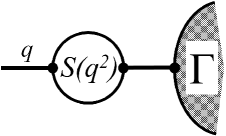
Figure 1: One loop insertion in external line of the S-matrix graph. The RP’s for $\Sigma(\kappa)$ should be taken according to 20 and 22.

At this point it seems me useful to formulate compactly the sequence of steps needed to perform the 1-loop renormalization of a given S-matrix graph. It looks as follows.

1. Draw the S-matrix graph $G$ under consideration. This should be done in accordance with Feynman rules that correspond to the initial effective Lagrangian. Select its 1PI one-loop subgraphs. (It is these subgraphs that are necessary and sufficient for renormalization).

2. Perform the reduction of all internal lines of the 2-leg subgraph $S(r^{2})$ selected at the previous step. This results in the sum of subgraphs of the same loop order $l=1$ as the initial ones. The loop numbers of these new subgraphs (we need to preserve the initial loop counting rules!) should be computed as the sums of the number of explicitly drawn loops plus the loop index (equal to 1) of the formally pointlike secondary vertex constructed from the coupling constants of the completely reduced subgraph $\Sigma(r^{2})$ (so-called secondary vertex of the one-loop level (see AVVV2 )).

3. Add the relevant one-loop counterterms. Keep in mind that the secondary vertices of one-loop level look precisely like the one-loop counterterms. Unite both series. The result is nothing but a new (redefined) counterterm series.

4. Impose the relevant (minimal!) RP’s – the result will be the correctly renormalized one-loop two-leg graph.

The advance of the above-described approach is obvious: one has no need in formulating the non-minimal RP’s for the one-loop 2-leg subgraphs!

Clearly, the same logic applies to the case when we consider the effect caused by the insertion of the two-leg one loop graph $S(r^{2})$ in internal line (see the graph $G$ in the left side of Fig. 2). It is clearly visible that the reduction of both lines $r$ (this does not change the analytical expression of the graph $G$!) leads to a separation of the initial graph into three parts. Only one of these parts requires knowledge of the one loop 2-leg graph $S(r^{2})$; two others relate to the next steps of the renormalization (3-, 4, …, n-leg graphs). This part is presented by the graph $A$, where the 2-leg subgraph is precisely $\Sigma(r^{2})$. The graphs $B$ and $C$ should be renormalized at next steps!

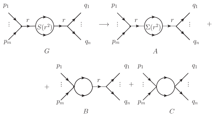
Figure 2: The reduction of the lines $r$ of the graph $G$ that follows from the Feynman rules based on the original effective Lagrangian. I do not show the relevant numerical coefficients in front of graphs $A$, $B$ and $C$ because they have no relation to the discussion of the topological structure. The dotted lines $r$ are minimal because the adjacent vertices are implied minimal with respect to these lines. The solid lines correspond to the sums of contributions of both kinds – minimal and nonminimal.

That is why (as have been explained above) one can introduce the alternative (“analytical”) definition of what is irreducibility: graphical (G1PI) versus analytical (A1PI) reducibility.

It might be useful to analyze the process of reduction of the simple (undressed) internal line. This point has been discussed already in papers AVVV2 and KSAVVV2 which I refer the reader to.

What is the essence of the above analysis? The thing is that for the renormalization of a given graph it is necessary (and sufficient) to renormalize all its 1PI subgraphs. In the case when we rely on the G1PI concept we would need to fix the non-minimal counterterms (just because the subgraphs may be non-minimal). In contrast, when all the lines of the graph in question have been reduced (the graph is made minimal), all its subgraphs turn out minimal and one only needs to fix the minimal counterterms. This confirms the general logical line described in AVVV2 , KSAVVV2 .

References

- (1) Vladimir V. Vereshagin, Phys. Rev. D 89, 125022 (2014).
- (2) A. Vereshagin and V. Vereshagin, Phys. Rev. D 69, 025002 (2004).
- (3) S. Weinberg, Physica 96A, 327 (1979).
- (4) S. Weinberg, The Quantum Theory of Fields, Vol. 1, (Cambridge University Press, Cambridge, 1996).
- (5) K. Semenov-Tian-Shansky, A. Vereshagin, and V. Vereshagin, Phys. Rev. D 73, 025020 (2006).
-
(6)
S. Weinberg, in
General Relativity – An Einstein Centenary Survey,
ed. by S. W. Hawking and W. Israel (Cambridge University Press, Cambridge, 1979). - (7) R. E. Kallosh and I. V. Tyitin, Sov. J. Nucl. Phys. 17, 98 (1973).
- (8) D. Chicherin, V. Gorbenko, and V. Vereshagin, Phys. Rev. D 84, 105003 (2011).
- (9) J. Gomis and S. Weinberg, Nucl.Phys. B469, 473 (1996).
- (10) Bogoliubov, N. N. and Shirkov, D. V. Introduction to the Theory of Quantized Fields. 3rd edition, Wiley, New York 1980.
- (11) M. E. Peskin and D. V. Schroeder, Quantum Field Theory (Addison-Wesley, NY, 1997).
- (12) Vladimir V. Vereshagin, Phys. Rev. D 55, number 9, 5349 (1997).
- (13) J. C. Collins, Renormalization (Cambridge Univ. Press, Cambridge, 1984).
-
(14)
A. N. Vasiliev,
The field theoretic renormalization group in
critical behavior theory and stochastic dynamics, (CRS Press LLC, 2004). - (15) M. Veltman, Physica, 29, 186 (1963).
- (16) S. Weinberg, Phys. Rev. 118, 838 (1960).