Large $h\to bs$ in generic two-Higgs-doublet models

Abstract

We investigate the possible size of $h\to bs$ in two-Higgs-doublet models with generic Yukawa couplings. Even though the corresponding rates are in general expected to be small due to the indirect constraints from $B_{s}\to\mu^{+}\mu^{-}$ and $B_{s}$–$\overline{B}_{s}$ mixing, we find regions in parameter space where $h\to bs$ can have a sizable branching ratio well above 10%. This requires a tuning of the neutral scalar masses and their couplings to muons, but then all additional constraints such as $B\to X_{s}\gamma$, $(g-2)_{\mu}$, and $h\to\mu^{+}\mu^{-}$ are satisfied. In this case, $h\to bs$ can be a relevant background in $h\to b\bar{b}$ searches and vice versa due to the imperfect $b$-tagging purity. Furthermore, if $h\to bs$ is sizeable, one expects two more scalar resonances in the proximity of $m_{h}$. We briefly comment on other flavour violating Higgs decays and on the 95 GeV $\gamma\gamma$ resonance within generic two-Higgs-doublet models.

I Introduction

The possibility of flavour-changing decays of the Brout–Englert–Higgs boson $h$ (Higgs for short in the following) has been discussed for a long time as a possible signal for physics beyond the Standard Model (SM) McWilliams:1980kj ; Shanker:1981mj ; Han:2000jz ; Giudice:2008uua ; Goudelis:2011un ; Harnik:2012pb ; Blankenburg:2012ex . Indirect constraints on these couplings come from flavour-changing neutral-current observables. In many analyses one follows an effective-field-theory approach in which one assumes that only the couplings of the SM-like Higgs to fermions are modified and derives constraints on these couplings from low-energy processes Harnik:2012pb ; Blankenburg:2012ex . This leads one to conclude that no flavour-changing Higgs decays can be observable at the LHC, with the possible exception of $h\to\tau e$ and $h\to\tau\mu$ Blankenburg:2012ex ; Harnik:2012pb . This is a dangerous conclusion because the very existence of flavour-changing Higgs couplings in a renormalizable SM extension implies additional states which posses flavour-changing couplings as well. The indirect constraints from flavour-changing neutral currents and rare decays are thus inherently model-dependent and can be decoupled from Higgs decays. This generically involves finetuning of the mass spectrum and couplings of the additional states, but opens the way for some new channels to look for physics beyond the SM.

In this article we will study the arguably simplest SM extension that can lead to flavour-changing couplings of the SM-like Higgs: the two-Higgs-Doublet Model (2HDM) with generic Yukawa couplings, i.e. type III. After computing the effects in $B_{s}$–$\overline{B}_{s}$ mixing, $B_{s}\to\mu^{+}\mu^{-}$ and $b\to s\gamma$, we identify regions of parameter space that can lead to sizable decay rates of $h\to bs$ (upwards of 10%) which are potentially observable at the LHC, hopefully motivating dedicated searches. This is particularly relevant now that the largest Higgs decay mode, $h\to b\bar{b}$, has finally been observed ATLAS:2017bic ; Sirunyan:2017elk , rendering it background for $h\to bs$. While not the focus of our work, we stress that the additional neutral states ($H$ or $A$) can easily have even larger flavour-violating branching ratios, so general resonance searches for $bs$ final states are encouraged as well.

The rest of this article is structured as follows: in Sec. II we set up our 2HDM notation. In Sec. III we discuss the main observables that could invalidate large $h\to bs$ rates and identify ways to circumvent their constraints. Sec. IV deals with direct searches for the new scalars at colliders, pointing out their main production and decay channels. We comment on different choices of bases for the 2HDM in Sec. V. Finally, we conclude in Sec. VI and provide an outlook for other rare Higgs decays. Appendix A provides one-loop formulae relevant for $b\to s\gamma$.

II Type-III 2HDM

Our starting point is the 2HDM with generic couplings to fermions (type III) and a CP conserving scalar potential Branco:2011iw . In the Higgs basis Georgi:1978ri ; Lavoura:1994fv ; Botella:1994cs in which only one doublet acquires a vacuum expectation value (using notation close to Ref. Davidson:2016utf ) we have

$$\Phi_{1}=\begin{pmatrix}G^{+}\\ \frac{v+H_{1}^{0}+iG^{0}}{\sqrt{2}}\end{pmatrix}, \Phi_{2}=\begin{pmatrix}H^{+}\\ \frac{H_{2}^{0}+iA}{\sqrt{2}}\end{pmatrix},$$ (1)

with $v\simeq 246\,\mathrm{GeV}$, the Goldstone bosons $G^{0,+}$, and the physical CP-odd scalar $A$. Assuming that CP is conserved in the scalar potential, the CP-even mass eigenstates are

$$h =H_{1}^{0}\sin(\beta-\alpha)+H_{2}^{0}\cos(\beta-\alpha)\,,$$ (2)

$$H =H_{1}^{0}\cos(\beta-\alpha)-H_{2}^{0}\sin(\beta-\alpha)\,,$$ (3)

where we defined the mixing angle as $\beta-\alpha$ for easier comparison with the well-known type-I/II/X/Y 2HDM. We will abbreviate $s_{\beta\alpha}\equiv\sin(\beta-\alpha)$, $c_{\beta\alpha}\equiv\cos(\beta-\alpha)$, and $t_{\beta\alpha}\equiv\tan(\beta-\alpha)$ below.

In the physical basis with diagonal fermion mass matrices the Yukawa couplings are given by

$$\begin{split}-\mathcal{L}_{Y}&=\sum_{f=u,d,\ell}\left[\overline{f}\left(y^{f}s_{\beta\alpha}+(\varepsilon^{f}P_{R}+{\varepsilon^{f}}^{\dagger}P_{L})c_{\beta\alpha}\right)f\,h\right.\\ &\quad+\overline{f}\left(y^{f}c_{\beta\alpha}-(\varepsilon^{f}P_{R}+{\varepsilon^{f}}^{\dagger}P_{L})s_{\beta\alpha}\right)f\,H\\ &\quad+\left.i\eta_{f}\,\overline{f}\left(\varepsilon^{f}P_{R}-{\varepsilon^{f}}^{\dagger}P_{L}\right)f\,A\right]\\ &\quad+\sqrt{2}\left[\overline{u}\left(V\varepsilon^{d}P_{R}-{\varepsilon^{u}}^{\dagger}VP_{L}\right)d\,H^{+}+\text{h.c.}\right]\\ &\quad+\sqrt{2}\left[\overline{\nu}\left(\varepsilon^{\ell}P_{R}\right)\ell\,H^{+}+\text{h.c.}\right],\end{split}$$ (4)

where $\eta_{d,\ell}=1=-\eta_{u}$ and $V$ is the Cabibbo–Kobayashi–Maskawa (CKM) matrix. $(y^{f})_{ij}=\delta_{ij}m_{j}^{f}/v$ are the standard (diagonal) SM Yukawa couplings, while $\varepsilon^{u,d,\ell}$ are arbitrary complex $3\times 3$ matrices in flavour space. Off-diagonal elements in $\varepsilon^{f}$ lead to flavour-changing Higgs couplings. For our channel of interest, $h\to\overline{b}s+b\overline{s}$, we have

$$\Gamma(h\to bs)\simeq\frac{3c_{\beta\alpha}^{2}m_{h}}{8\pi}(|\varepsilon_{23}^{d}|^{2}+|\varepsilon_{32}^{d}|^{2})\left(1-\frac{m_{b}^{2}}{m_{h}^{2}}\right)^{2}.$$ (5)

Note that this expression is valid at tree level; next-to-leading order QCD corrections might increase the decay rate by $10$–$20\%$ Barenboim:2015fya . However, since we are interested in an order of magnitude estimate, such corrections are not of particular importance here. The resulting branching ratio is then

$$\mathrm{BR}(h\to bs)=\frac{\Gamma(h\to bs)}{\Gamma(h\to bs)+s_{\beta\alpha}^{2}\Gamma_{\mathrm{SM}}}\,,$$ (6)

with $\Gamma_{\mathrm{SM}}\simeq 4.1\,\mathrm{MeV}$ and assuming all $\varepsilon^{u,d,\ell}$ to be zero, except of course those for $h\to bs$. Note that a branching ratio of $h\to bs$ of $1\%$ ($10\%$) requires $\varepsilon^{d}_{23,32}$ couplings of order $0.02$ ($0.06$), assuming $c_{\beta\alpha}=0.1$.

So far no searches for $h\to bs$ have been performed, making it difficult to assess the sensitivity. The channel $h\to b\bar{b}$, which has a large SM branching ratio of $58\%$, has only recently been observed ATLAS:2017bic ; Sirunyan:2017elk despite its better $b$-tagging possibilities compared to $h\to bs$. Nevertheless, we can obtain a model-independent limit on $\Gamma(h\to bs)$ of $1.1\,\mathrm{GeV}$ Sirunyan:2017exp , corresponding roughly to the CMS energy resolution. This is still almost three orders of magnitude above the SM value $\Gamma_{\mathrm{SM}}$, and thus still allows for $\mathrm{BR}(h\to bs)\sim 1$. A more intricate upper limit on the Higgs width can be obtained by comparing on- and off-shell cross sections, as proposed in Ref. Caola:2013yja . A recent CMS analysis of run-1 data along these lines obtains $\Gamma_{h}<13\,\mathrm{MeV}$ Khachatryan:2016ctc . While it cannot be claimed to be a model-independent limit Englert:2014aca , it should hold true in our scenario with $c_{\beta\alpha}\ll 1$, seeing as $h$ becomes arbitrarily SM-like. Naively applying $\Gamma_{h}<13\,\mathrm{MeV}$ on our model and using $c_{\beta\alpha}\leq 0.55$ as a very conservative bound (see below), this implies $\mathrm{BR}(h\to bs)\lesssim 78\%$; for $c_{\beta\alpha}\ll 1$ the limit is $\mathrm{BR}(h\to bs)\lesssim 68\%$. This is obviously still very large and can most likely be improved by a direct search for $h\to bs$. We will use this as a conservative limit in the following.

Stronger limits can be obtained from global fits to observed Higgs production and decay channels, seeing as a large $\Gamma(h\to bs)$ would reduce all measured Higgs branching ratios and hence require a larger production cross section to obtain the same rates. An analysis of this type with LHC run-1 data was performed in Ref. Khachatryan:2016vau and lead to the $95\%$ C.L. limit $\mathrm{BR}(h\to\text{new})<34\%$ on any new decay channels, including $bs$. This is a factor of two stronger than the limit from the Higgs width, in part because it is based on a combination of ATLAS and CMS data and makes use of more search channels. We will also show this limit in the following, but stress that it should be taken with a grain of salt; global-fit limits are very indirect and depend strongly on the assumptions one puts in. With the many parameters available in a type-III 2HDM, it is conceivable that the limit could be weakened by increasing some parameters relevant to Higgs production. A dedicated search for $h\to bs$ will yield far more direct constraints and should always be preferred to global-fit limits.

The goal of our article is to show that a sizable branching ratio for $h\to bs$ is possible, even up to the conservative limit of $68\%$. To simplify the analysis we will set as many entries of $\varepsilon^{f}$ to zero as possible, i.e. $\varepsilon^{u,d,\ell}_{ij}=0$ is the starting point of our investigation. In this limit, we can obtain bounds on the masses and on the mixing angle $\beta-\alpha$ by comparison with the type-I 2HDM (in the limit $\tan(\beta)\to\infty$, i.e. $\beta\to\pi/2$, identifying our $c_{\beta\alpha}$ with the type-I $\sin(\alpha)=\cos(\pi/2-\alpha)$). This gives the rather weak bound $|c_{\beta\alpha}|\lesssim 0.55$ from LHC run-1 Higgs measurements Dorsch:2016tab ; Marcellini:2017nwk . In the limit $c_{\beta\alpha}\to 0$, the new scalars become completely fermiophobic and the model resembles the Inert Higgs Doublet (IDM), with a $\mathbb{Z}_{2}$ symmetry that only allows the new scalars to be produced in pairs. This $\mathbb{Z}_{2}$ is of course broken in the scalar potential and by $c_{\beta\alpha}\neq 0$, but it allows us to use well-known limits on IDM. In particular, LEP constraints on the $Z$ and $W$ widths approximately require

$$m_{A}+m_{H}\geq m_{Z}\,, m_{H^{+}}+m_{A,H}\geq m_{W}\,,$$ (7)

while LEP-II excludes $m_{H^{+}}<70\,\mathrm{GeV}$ and also restricts the $m_{A}$–$m_{H}$ parameter space Lundstrom:2008ai . Additional bounds come from LHC searches, which most importantly constrain the masses below $m_{h}/2$ Belanger:2015kga ; Datta:2016nfz . The Peskin–Takeuchi parameters $S$ and $T$ also provide constraints, unless the mass spectrum satisfies $m_{A}\simeq m_{H^{+}}$ (for $\Delta T\simeq 0$) and $m_{A}\simeq m_{H}\simeq m_{H^{+}}$ (for $\Delta S\simeq 0$) Barbieri:2006dq ; Haber:2010bw ; Arhrib:2012ia . All in all, the fermiophobic limit still allows for new-scalar masses around $100\,\mathrm{GeV}$, depending on the hierarchy. Turning on the mixing angle $\beta-\alpha$ will significantly affect the limits on $m_{H}$ as it opens up gluon fusion, diphoton decay, etc., to be discussed below.

III Observables

Since we are interested in $h\to bs$ we will use the ansatz

$$\varepsilon^{d}=\begin{pmatrix}0&0&0\\ 0&0&\varepsilon_{23}^{d}\\ 0&\varepsilon_{32}^{d}&0\end{pmatrix}, \varepsilon^{\ell}=\begin{pmatrix}0&0&0\\ 0&\varepsilon_{\mu\mu}^{\ell}&0\\ 0&0&0\end{pmatrix}, \varepsilon^{u}=0\,,$$ (8)

where in addition to $\varepsilon_{23,32}^{d}$ we also allow for non-zero values of $\varepsilon_{\mu\mu}^{\ell}$ because this entry is important for $B_{s}\to\mu^{+}\mu^{-}$. In addition to $B_{s}\to\mu^{+}\mu^{-}$, the most relevant constraints originate from $B_{s}$–$\overline{B}_{s}$ mixing and $B\to X_{s}\gamma$.

These channels were also discussed in the MSSM (i.e. type-II 2HDM), where the $h\to bs$ branching ratio was found to be tiny Barenboim:2015fya ; Gomez:2015duj . Here it is important to discuss the difference of our analysis to the MSSM. Even though at the loop-level non-decoupling effects in the MSSM induce non-holomorphic Higgs couplings Hempfling:1993kv ; Hall:1993gn ; Carena:1994bv ; Noth:2008tw ; Hofer:2009xb ; Crivellin:2010er ; Crivellin:2011jt ; Crivellin:2012zz (making it a type-III 2HDM), these effects are only corrections to the type-II structure. Therefore, the strong bounds from direct LHC searches for additional Higgs bosons as well as the stringent bounds from $b\to s\gamma$ on the charged Higgs mass of around 570 GeV apply Misiak:2017bgg . Furthermore, in the MSSM the angle $\alpha$ is directly related to $m_{A}\simeq m_{H^{+}}$, rendering it small and further suppressing $h\to bs$.

III.1 $B_{s}$–$\overline{B}_{s}$ mixing

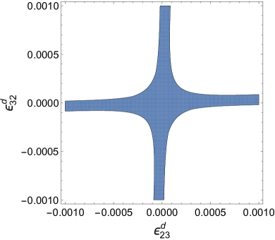
Figure 1: Allowed regions in the $\varepsilon^{d}_{23}$–$\varepsilon^{d}_{32}$ plane for $m_{H}=150\,\mathrm{GeV}$ and $c_{\beta\alpha}=0.1$, requiring that the 2HDM contribution to $B_{s}$–$\overline{B}_{s}$ mixing should not exceed 10% compared to the SM which is of the order of the uncertainty in the lattice calculation of the matrix elements. Here we scanned over $m_{A}$ from 100 to 200 GeV. Note that the dependence on $c_{\beta\alpha}$ is very weak. As one can see, in order to get potentially large effects in $h\to bs$, either $\varepsilon^{d}_{23}$ or $\varepsilon^{d}_{32}$ must be very small.

The $\Delta F=2$ process $B_{s}$–$\overline{B}_{s}$ mixing is unavoidably modified already at tree-level if $h\to bs$ has a non-vanishing rate. To describe this process we use the effective Hamiltonian (see for example Becirevic:2001jj )

$$\mathcal{H}_{\mathrm{eff}}=\sum_{j=1}^{5}C_{j}O_{j}+\sum_{j=1}^{3}C_{j}^{\prime}O_{j}^{\prime}+\text{h.c.}\,,$$ (9)

where non-vanishing Wilson coefficients are generated for the three operators

$$O_{2}^{(\prime)} \equiv(\overline{s}_{A}P_{L,(R)}b_{A})(\overline{s}_{B}P_{L,(R)}b_{B})\,,$$ (10)

$$O_{4} \equiv(\overline{s}_{A}P_{L}b_{A})(\overline{s}_{B}P_{R}b_{B})\,,$$ (11)

with $A$ and $B$ being colour indices. At tree level, we obtain the Wilson coefficients Crivellin:2013wna

$$C_{2} =-\frac{(\varepsilon^{d\,\star}_{32})^{2}}{2}\left[\frac{c_{\beta\alpha}^{2}}{m_{h}^{2}}+\frac{s_{\beta\alpha}^{2}}{m_{H}^{2}}-\frac{1}{m_{A}^{2}}\right],$$ (12)

$$C_{2}^{\prime} =-\frac{(\varepsilon^{d}_{23})^{2}}{2}\left[\frac{c_{\beta\alpha}^{2}}{m_{h}^{2}}+\frac{s_{\beta\alpha}^{2}}{m_{H}^{2}}-\frac{1}{m_{A}^{2}}\right],$$ (13)

$$C_{4} =-(\varepsilon^{d\,\star}_{32}\varepsilon^{d}_{23})\left[\frac{c_{\beta\alpha}^{2}}{m_{h}^{2}}+\frac{s_{\beta\alpha}^{2}}{m_{H}^{2}}+\frac{1}{m_{A}^{2}}\right].$$ (14)

Computing the $B_{s}$–$\overline{B}_{s}$ mass difference by inserting the matrix elements together with the corresponding bag factor and taking into account the renormalization group evolution Becirevic:2001jj , we show the result in Fig. 1. Here, one can see that $\varepsilon^{d}_{23}$ ($\varepsilon^{d}_{32}$) can only be sizable if $\varepsilon^{d}_{32}$ ($\varepsilon^{d}_{23}$) is close to zero. In fact, one can avoid any effect in $B_{s}$–$\overline{B}_{s}$ mixing by setting

$$m_{A}=\frac{m_{h}m_{H}}{\sqrt{m_{h}^{2}s_{\beta\alpha}^{2}+m_{H}^{2}c_{\beta\alpha}^{2}}}\,, \varepsilon^{d\,\star}_{32}\varepsilon^{d}_{23}=0\,.$$ (15)

This in particular implies that $m_{A}$ is between $m_{h}$ and $m_{H}$, so neither the heaviest nor the lightest neutral scalar. Even with all new-physics Wilson coefficients vanishing at tree level, loop contributions, including those with $H^{+}$, will generate additional contributions. However, since all contributions interfere, this effect is significantly suppressed compared to the tree-level exchange and can always be cancelled by a small modification of Eq. (15). We can hence eliminate any new-physics effect in $B_{s}$–$\overline{B}_{s}$ mixing using Eq. (15) while keeping either $\varepsilon^{d}_{23}$ or $\varepsilon^{d}_{32}$ large.

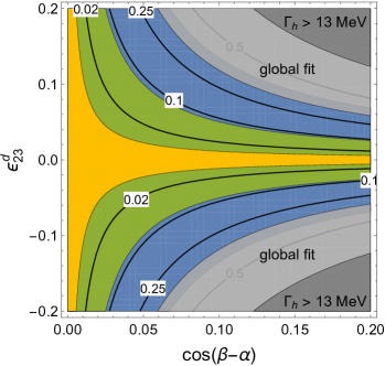
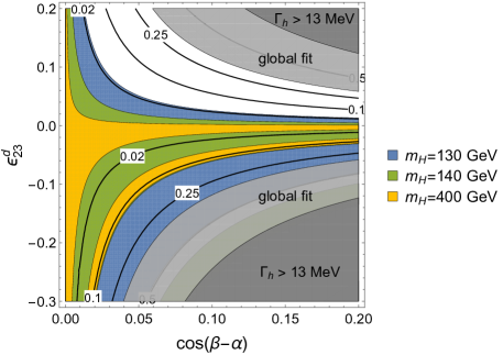
Figure 2: $\mathrm{BR}(h\to bs)$ contours and the allowed $2\sigma$ regions from $B_{s}\to\mu^{+}\mu^{-}$. Left: setting all $\varepsilon^{f}=0$ except for $\varepsilon^{d}_{23}$, with $m_{A}$ given by Eq. (15). Right: Same as left plot but with non-zero $\varepsilon_{\mu\mu}^{\ell}$ given by Eq. (23) instead. The darker gray region is excluded by the upper limit on the total decay width of the Higgs of 13 MeV Khachatryan:2016ctc and the lighter gray region is excluded by the global-fit constraint $\mathrm{BR}(h\to\rm{anything})<34\%$ Khachatryan:2016vau .

III.2 $B_{s}\to\mu^{+}\mu^{-}$

The $\varepsilon^{d}_{23,32}$ couplings necessary for $h\to bs$ also induce a modification of $B_{s}\to\mu^{+}\mu^{-}$ at tree level, because by construction all three neutral scalars couple to $bs$, and at least two scalars also couple to $\mu^{+}\mu^{-}$. The effective Hamiltonian takes the form Crivellin:2013wna

$$\begin{split}\mathcal{H}_{\mathrm{eff}}^{B_{s}\to\mu\mu}&=-\frac{G_{F}^{2}m_{W}^{2}}{\pi^{2}}\left[C_{A}O_{A}+C_{S}O_{S}+C_{P}O_{P}\right.\\ &\quad\left.+C_{A}^{\prime}O_{A}^{\prime}+C_{S}^{\prime}O_{S}^{\prime}+C_{P}^{\prime}O_{P}^{\prime}\right]+\text{h.c.},\end{split}$$ (16)

with

$$O_{A} \equiv(\overline{b}\gamma_{\alpha}P_{L}s)(\overline{\mu}\gamma^{\alpha}\gamma_{5}\mu)\,,$$ (17)

$$Q_{S} \equiv(\overline{b}P_{L}s)(\overline{\mu}\mu)\,,$$ (18)

$$Q_{P} \equiv(\overline{b}P_{L}s)(\overline{\mu}\gamma_{5}\mu)\,.$$ (19)

$O_{X}^{\prime}$ are obtained from $O_{X}$ by replacing $P_{L}$ with $P_{R}$. The branching ratio then reads Crivellin:2013wna

$$\mathrm{BR}(B_{s}\to\mu^{+}\mu^{-})=\frac{G_{F}^{4}m_{W}^{4}}{8\pi^{5}}\sqrt{1-\frac{4m_{\mu}^{2}}{M_{B_{s}}^{2}}}M_{B_{s}}f_{B_{s}}^{2}m_{\mu}^{2}\tau_{B_{s}}$$

$$\qquad\times\left[\left|\frac{M_{B_{s}}^{2}(C_{P}-C_{P}^{\prime})}{2m_{\mu}(m_{b}+m_{s})}-(C_{A}-C_{A}^{\prime})\right|^{2}\right.$$

$$\qquad\qquad+\left.\left|\frac{M_{B_{s}}^{2}(C_{S}-C_{S}^{\prime})}{2m_{\mu}(m_{b}+m_{s})}\right|^{2}\left(1-\frac{4m_{\mu}^{2}}{M_{B_{s}}^{2}}\right)\right]\,,$$ (20)

experimentally determined to be $\left(2.8^{+0.7}_{-0.6}\right)\times 10^{-9}$ CMS:2014xfa . The SM yields only one non-zero Wilson coefficient, $C_{A}^{\text{SM}}\sim-V_{ts}V_{tb}^{*}$, while our neutral scalars induce

$$\begin{split}C_{S}-&C_{S}^{\prime}=\frac{\pi^{2}}{G_{F}^{2}m_{W}^{2}}\left[\frac{i}{m_{A}^{2}}\Im(\varepsilon_{\mu\mu}^{\ell})\left(\varepsilon_{23}^{d\,\star}+\varepsilon_{32}^{d}\right)\right.\\ &+\frac{c_{\beta\alpha}}{m_{h}^{2}}\left(y_{\mu\mu}^{\ell}s_{\beta\alpha}+\Re(\varepsilon_{\mu\mu}^{\ell})c_{\beta\alpha}\right)\left(\varepsilon_{23}^{d\,\star}-\varepsilon_{32}^{d}\right)\\ &\left.-\frac{s_{\beta\alpha}}{m_{H}^{2}}\left(y_{\mu\mu}^{\ell}c_{\beta\alpha}-\Re(\varepsilon_{\mu\mu}^{\ell})s_{\beta\alpha}\right)\left(\varepsilon_{23}^{d\,\star}-\varepsilon_{32}^{d}\right)\right],\end{split}$$ (21)

$$\begin{split}C_{P}-&C_{P}^{\prime}=\frac{\pi^{2}}{G_{F}^{2}m_{W}^{2}}\left[\frac{1}{m_{A}^{2}}\Re(\varepsilon_{\mu\mu}^{\ell})\left(\varepsilon_{23}^{d\,\star}+\varepsilon_{32}^{d}\right)\right.\\ &\left.+i\left(\frac{c_{\beta\alpha}^{2}}{m_{h}^{2}}+\frac{s_{\beta\alpha}^{2}}{m_{H}^{2}}\right)\Im(\varepsilon_{\mu\mu}^{\ell})\left(\varepsilon_{23}^{d\,\star}-\varepsilon_{32}^{d}\right)\right].\end{split}$$ (22)

First of all note that one cannot avoid effects here by setting $\varepsilon_{32}^{d}=\pm\varepsilon_{23}^{d\,\star}$ due to the constraints from $B_{s}$–$\overline{B}_{s}$ mixing. Adjusting $\varepsilon^{\ell}_{\mu\mu}$ allows one to eliminate the muon coupling of at most one of the neutral scalars, leaving the other two contributing to $B_{s}\to\mu^{+}\mu^{-}$ at tree level. Setting for example $\varepsilon_{\mu\mu}^{\ell}=0$ gives $C_{P}-C_{P}^{\prime}=0$ and $C_{S}-C_{S}^{\prime}\propto(1/m_{h}^{2}-1/m_{H}^{2})\left(\varepsilon_{23}^{d\,\star}-\varepsilon_{32}^{d}\right)$, which can only be made small for $m_{H}\sim m_{h}$ with our ansatz from Eq. (15). As can be seen in Fig. 2 (left), this is already sufficient to obtain $\mathrm{BR}(h\to bs)=\mathcal{O}(10\%)$ while satisfying the experimental $B_{s}\to\mu^{+}\mu^{-}$ result within $2\sigma$.

An even better ansatz is to choose a (real) $\varepsilon_{\mu\mu}^{\ell}$ such that $C_{S}-C_{S}^{\prime}=0$, as this allows for new-physics contributions interfering with the SM Wilson coefficient $C_{A}$. The required coupling for $C_{S}-C_{S}^{\prime}=0$ is

$$\varepsilon_{\mu\mu}^{\ell}=\frac{c_{\beta\alpha}s_{\beta\alpha}\left(m_{h}^{2}-m_{H}^{2}\right)}{c_{\beta\alpha}^{2}m_{H}^{2}+s_{\beta\alpha}^{2}m_{h}^{2}}y_{\mu\mu}^{\ell}\,,$$ (23)

which gives, using also Eq. (15),

$$C_{P}-C_{P}^{\prime}=\frac{\pi^{2}y_{\mu\mu}^{\ell}c_{\beta\alpha}s_{\beta\alpha}}{G_{F}^{2}m_{W}^{2}}\left(\frac{1}{m_{H}^{2}}-\frac{1}{m_{h}^{2}}\right)\left(\varepsilon_{23}^{d\,\star}+\varepsilon_{32}^{d}\right).$$ (24)

The most obvious way to eliminate the new-physics effect here is to choose $m_{H}=m_{h}$, which also implies $m_{A}=m_{h}$ with Eq. (15). Another possibility is to pick the phase of $\varepsilon_{23,32}^{d}$ in such a way that it induces destructive interference with the SM contribution $C_{A}$, which will soften the limits and allow for larger $h\to bs$, see Fig. 2 (right). The largest possible $h\to bs$ values arise when $C_{P}-C_{P}^{\prime}$ destructively interferes with $C_{A}^{\text{SM}}$, while keeping $\mathrm{BR}(B_{s}\to\mu^{+}\mu^{-})$ close to its SM value. Indeed, if we impose the condition

$$\frac{M_{B_{s}}^{2}(C_{P}-C_{P}^{\prime})}{2m_{\mu}(m_{b}+m_{s})}-C_{A}^{\text{SM}}\stackrel{{\scriptstyle!}}{{=}}+C_{A}^{\text{SM}}\,,$$ (25)

then all observables in $B_{s}\to\mu^{+}\mu^{-}$ will remain exactly at their SM values, as we are effectively just flipping the sign of the SM contribution, which is unphysical (see, for example, Refs. Blake:2016olu ; Fleischer:2017yox ). The above relation can be immediately solved for $\varepsilon_{23,32}^{d}$

$$\varepsilon_{23}^{d\,\star}+\varepsilon_{32}^{d}=\frac{4G_{F}^{2}m_{W}^{2}m_{b}m_{\mu}C_{A}^{\text{SM}}m_{h}^{2}m_{H}^{2}}{\pi^{2}c_{\beta\alpha}s_{\beta\alpha}y_{\mu\mu}^{\ell}M_{B_{s}}^{2}(m_{h}^{2}-m_{H}^{2})}\,,$$ (26)

where $m_{b}$ should now be evaluated at the scale $m_{H}$ to take the running of $C_{P}-C_{P}^{\prime}$ into account Crivellin:2013wna .

To reiterate, choosing masses and couplings according to Eqs. (15), (23), (26) allows us to keep all $B_{s}$–$\overline{B}_{s}$ and $B_{s}\to\mu^{+}\mu^{-}$ observables at their SM values, even though $h\to bs$ can be large. The only free relevant parameters left are $c_{\beta\alpha}$ and $m_{H}$, so we can show $h\to bs$ as a function of $m_{H}$, see Fig. 3. As expected, the region $m_{H}\sim m_{h}$ allows for the largest $h\to bs$ rates due to the cancellation in $C_{P}-C_{P}^{\prime}$ in Eq. (24). However, even for $m_{h}\ll m_{H}$ and $c_{\beta\alpha}\ll 1$ one can obtain $\mathrm{BR}(h\to bs)\simeq 10\%$.

As an aside, Eq. (26) is the only expression so far that depends on the quark flavour, via $C_{A}^{\text{SM}}\sim V_{ts}V_{tb}^{*}$. All our results can thus be easily translated to the case $h\to bd$, with $\Gamma(h\to bd)/\Gamma(h\to bs)\simeq|V_{td}/V_{ts}|^{2}\simeq 0.05$ in the maximum-cancellation region. A large $h\to bd$ rate above the percent level thus requires $m_{H}\sim m_{A}\sim m_{h}$ if $B_{d}$–$\bar{B}_{d}$ mixing and $B\to\mu^{+}\mu^{-}$ are to be kept around their SM values. Hence, larger fine-tuning is needed.

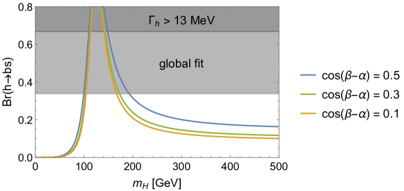
Figure 3: $\mathrm{BR}(h\to bs)$ vs. $m_{H}$ for our ansatz from Eqs. (15), (23), (26) for different values of $c_{\beta\alpha}$. Note that for degenerate masses of the neutral scalars $h\to bs$ is in principle unbounded.

III.3 $B\to X_{s}\gamma$

At loop level our new scalars unavoidably modify $B\to X_{s}\gamma$ Blake:2016olu , the relevant one-loop formulae can be found in App. A. Only the Wilson coefficients $C_{7}$ and $C_{8}$ are induced in our model. With our Eqs. (15), (23), (26), for the neutral scalars we find that $C_{8}=-3C_{7}$ depends only on $m_{H}$ but not on the mixing angle. We can thus predict the size of $C_{7}$ as a function of $m_{H}$ (or $\mathrm{BR}(h\to bs)$ with the help of Fig. 3). For $m_{H}$ in the region of interest for a large $h\to bs$, we find a tiny $|C_{7}|\simeq 2\times 10^{-3}$ ($2\times 10^{-6}$) for $\varepsilon_{32}^{d}=0$ ($\varepsilon_{23}^{d}=0$), far below the current limit Paul:2016urs . $B\to X_{s}\gamma$ is hence trivially compatible with a large $h\to bs$ in the region of parameter space under study here.

III.4 $B\to K\ell^{+}\ell^{-}$ and $B_{s}\to\tau^{+}\tau^{-}$

The decay $B_{s}\to\mu^{+}\mu^{-}$ is sensitive to the difference of the Wilson coefficients $C_{P,S}-C_{P,S}^{\prime}$, whereas $B\to K\mu^{+}\mu^{-}$ depends on their sum $C_{P,S}+C_{P,S}^{\prime}$ Bobeth:2007dw ; Becirevic:2012fy ; Hiller:2014yaa . With our ansatz from Eqs. (15), (23), (26), we have $C_{S}=C_{S}^{\prime}=0$ and either $C_{P}=0$ or $C_{P}^{\prime}=0$, depending on which $\varepsilon^{d}_{23,32}$ we set to zero. We thus unavoidably modify $B\to K\mu^{+}\mu^{-}$ at tree level. Using the results of Ref. Becirevic:2012fy , we checked that this effect is very small, keeping $B\to K\mu^{+}\mu^{-}$ close to the SM value. This means that our model cannot address the observed deviations from the SM prediction in current global fits to $b\to s\mu^{+}\mu^{-}$ observables Capdevila:2017bsm ; Altmannshofer:2017yso ; Hurth:2017hxg .

Similarly, one can expect an effect in $B\to K\tau^{+}\tau^{-}$ or $B_{s}\to\tau^{+}\tau^{-}$. Even though the effect is enhanced by $m_{\tau}/m_{\mu}$, the very weak experimental bounds on the branching ratio TheBaBar:2016xwe ; Aaij:2017xqt (several times $10^{-3}$) do not pose relevant constraints on our parameter space.

III.5 Anomalous Magnetic Moment of the Muon

The choice of $\varepsilon_{\mu\mu}^{\ell}$ in Eq. (23) reduces the coupling of $h$ to $\mu\mu$, but enhances the one of $H$ by a factor of few, and also couples $A$ and $H^{+}$ to muons. As a result, one could expect a modification of $(g-2)_{\mu}$, an observable that famously deviates from the SM value by around $3\sigma$ and can be explained in 2HDMs Iltan:2001nk ; Broggio:2014mna ; Crivellin:2015hha . However, the one-loop effect is still suppressed by the small muon mass. In addition, the usually dominant Barr–Zee contributions Barr:1990vd are also not important in our Higgs basis (with a minimal number of free parameters $\varepsilon^{f}$) since the couplings to heavy fermions (top, bottom or tau) are not enhanced for the heavy scalars. Furthermore, $B_{s}\to\mu^{+}\mu^{-}$ prefers nearly degenerate masses for $A$ and $H$, leading to a cancellation in the anomalous magnetic moment of the muon.

III.6 $B^{-}\to\mu\overline{\nu}$, $D_{s}^{-}\to\mu\overline{\nu}$, and $K^{-}\to\mu\overline{\nu}$

Concerning $H^{+}$ effects, the best channel is $B^{-}\to\mu\overline{\nu}$ (assuming $\varepsilon^{\ell}_{\tau\tau}=0$), with the rate

$$\frac{\mathrm{BR}(B^{-}\to\mu\overline{\nu})}{\mathrm{BR}(B^{-}\to\mu\overline{\nu})_{\text{SM}}}\simeq\left|1-\frac{m_{B^{-}}^{2}}{m_{\mu}m_{b}}\frac{V_{us}\varepsilon^{d}_{23}\varepsilon_{\mu\mu}^{\ell}}{\sqrt{2}G_{F}V_{ub}m_{H^{+}}^{2}}\right|^{2},$$ (27)

where $m_{b}$ is again to be evaluated at the scale $m_{H^{+}}$ to take the running of the Wilson coefficients into account. The predicted SM branching ratio $\mathrm{BR}(B^{-}\to\mu\overline{\nu})_{\text{SM}}\simeq 6\times 10^{-7}$ is small and not observed yet, but our new contribution could reach the current upper limit $\mathrm{BR}(B^{-}\to\mu\overline{\nu})<10^{-6}$ Aubert:2009ar . From Fig. 4 we see that the limits are rather weak and automatically satisfied in the region $m_{H^{+}}\sim m_{H}$.

Two other indirect channels are of potential interest: $D_{s}^{-}\to\mu\overline{\nu}$ and $K^{-}\to\mu\overline{\nu}$, the latter of which is suppressed but measured with more accuracy. We have

$$\frac{\mathrm{BR}(K^{-}\to\mu\overline{\nu})}{\mathrm{BR}(K^{-}\to\mu\overline{\nu})_{\text{SM}}}\simeq\left|1-\frac{m_{K^{-}}^{2}}{m_{\mu}m_{s}}\frac{V_{ub}\varepsilon^{d}_{32}\varepsilon_{\mu\mu}^{\ell}}{\sqrt{2}G_{F}V_{us}m_{H^{+}}^{2}}\right|^{2},$$ (28)

which gives much weaker bounds than $B^{-}\to\mu\nu$ before.

IV Collider Constraints

Having explored the indirect constraints that come with a large $h\to bs$ decay, let us briefly comment on possible collider searches.

IV.1 Charged Scalar

The charged scalar has barely played a role in any of the processes discussed so far, thanks to our ansatz for the $\varepsilon$ couplings in Eq. (8) together with Eq. (15). Its mass is hence a more-or-less free parameter, as long as we keep it close enough to $m_{A,H}$ to not induce too large $S$ and $T$ parameters. Let us briefly comment on the $H^{+}$ phenomenology beyond electroweak precision observables (see also Ref. Akeroyd:2016ymd for a recent review). Aside from gauge couplings, $H^{+}$ only couples according to Eq. (4):

$$-\mathcal{L}_{Y} =\sqrt{2}\left[\overline{u}\left(V\varepsilon^{d}P_{R}\right)d+\overline{\nu}\left(\varepsilon^{\ell}P_{R}\right)\ell\right]H^{+}+\text{h.c.},$$ (29)

where $\varepsilon^{\ell}$ contains only the non-zero entry $\varepsilon_{\mu\mu}^{\ell}$ and the quark couplings are determined by the matrix

$$V\varepsilon^{d}=\begin{pmatrix}0&V_{ub}\varepsilon_{32}^{d}&V_{us}\varepsilon_{23}^{d}\\ 0&V_{cb}\varepsilon_{32}^{d}&V_{cs}\varepsilon_{23}^{d}\\ 0&V_{tb}\varepsilon_{32}^{d}&V_{ts}\varepsilon_{23}^{d}\end{pmatrix}.$$ (30)

Since we impose $\varepsilon^{d\,\star}_{32}\varepsilon^{d}_{23}=0$ in order to satisfy limits from $B_{s}$–$\overline{B}_{s}$ mixing, the $H^{+}$ couples only either to $b$ or $s$ quarks. In particular, it does not contribute to $b\to s\gamma$. $\varepsilon^{d}_{23,32}$ is much bigger than the $\varepsilon_{\mu\mu}^{\ell}$ given by Eq. (23) for a sizeable $h\to bs$ rate, so the dominant coupling of $H^{+}$ is to quarks. If $H^{+}$ is lighter than the top quark, it can be produced in its decays:

If $\varepsilon^{d}_{32}=0$, the production channel is $t\to bH^{+}$, suppressed by $V_{ts}$, followed by $H^{+}\to\bar{b}c$ with branching ratio $\simeq 1$. This channel has been looked for Laurila:2017phk , with constraints around $|\varepsilon^{d}_{23}|\lesssim 2$ for $m_{H^{+}}$ between $90$ and $150\,\mathrm{GeV}$. This is still compatible with a large $h\to bs$ rate as long as $c_{\beta\alpha}$ is not too small ($c_{\beta\alpha}>0.1$). For completeness, we can replace $\varepsilon^{d}_{23}$ directly with the $h\to bs$ branching ratio $\mathrm{BR}_{h}^{bs}$ to predict

$$\frac{\Gamma(t\to bH^{+})}{m_{t}}\simeq\frac{|V_{ts}|^{2}s_{\beta\alpha}^{2}}{6c_{\beta\alpha}^{2}}\frac{\mathrm{BR}_{h}^{bs}}{1-\mathrm{BR}_{h}^{bs}}\frac{\Gamma_{h}^{\text{SM}}}{m_{h}}\left(1-\frac{m_{H^{+}}^{2}}{m_{t}^{2}}\right)^{2}.$$ (31)

If instead $\varepsilon^{d}_{23}=0$, the production channel will be $t\to sH^{+}$ with $\mathrm{BR}(H^{+}\to\bar{s}c)\simeq 1$. The rate can be obtained from Eq. (31) via $V_{ts}\to V_{tb}$, so this channel is enhanced by $|V_{tb}/V_{ts}|^{2}\simeq 580$ compared to the previous one. Since this final state has only been considered with the production channel $t\to bH^{+}$ Aad:2013hla ; Khachatryan:2015uua , we cannot obtain useful limits.

For $H^{+}$ masses above the top mass the typical search channel is $H^{+}\to tb$ ATLAS:2016qiq or $H^{+}\to\tau\nu$, which are suppressed or even zero in our scenario and hence not good signatures.

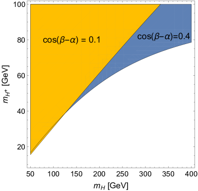
Figure 4: Allowed region from $B\to\mu\nu$ for our ansatz from Eqs. (15), (23), (26) with $\varepsilon^{d}_{32}=0$.

IV.2 Neutral Scalars

The neutral scalars $H$ and $A$ have large couplings to $bs$, but also the far easier to detect muon coupling exists. For $A$, the branching ratio is however very small,

$$\mathrm{BR}(A\to\mu^{+}\mu^{-})\simeq 2\times 10^{-4}c_{\beta\alpha}^{4}\frac{1-\mathrm{BR}_{h}^{bs}}{\mathrm{BR}_{h}^{bs}}\left(1-\frac{m_{H}^{2}}{m_{h}^{2}}\right)^{2},$$ (32)

especially in the region $m_{H}\sim m_{h}$ where the $h\to bs$ branching ratio $\mathrm{BR}_{h}^{bs}$ is largest. As a result, the best search channel is typically $A\to bs$. The same is true for $H$ in the limit $c_{\beta\alpha}\ll 1$, although a sizeable $c_{\beta\alpha}$ can lead to a large $H\to b\bar{b}$. With essentially only a large $bs$ coupling, $A$ can be produced at the LHC via the strange-quark sea, e.g. $sg\to bA$, followed by $A\to bs$ or $A\to\mu\mu$. Similar channels have been discussed in the past, see for example Refs. Dawson:2004nv ; Altmannshofer:2016zrn . For $H$, the $c_{\beta\alpha}$-suppressed gluon or vector-boson-fusion channels become available too, allowing for a search analogous to $h\to bs$.

A particularly interesting, albeit also $c_{\beta\alpha}$-suppressed, decay channel for $H,A$ is $H,A\to\gamma\gamma$. Recent $\sqrt{s}=13\,\mathrm{TeV}$ CMS limits for this signature can be found in Ref. CMS:2017yta , which also shows a small ($2.9\sigma$ local, $1.5\sigma$ global) excess around $m\simeq 95\,\mathrm{GeV}$. This would be an interesting value for $m_{H}$, as it can lead to $\mathrm{BR}(h\to bs)\sim 20\%$ (Fig. 3). With the couplings at hand, the cross section $pp\to H\to\gamma\gamma$ is simply too small for realistic values of $c_{\beta\alpha}$. However, the discussion so far assumed that all other entries $\varepsilon^{f}_{ij}$ except $\varepsilon^{d}_{23,32}$ are zero. Introducing extra couplings, in particular $\varepsilon^{u}_{33}$, enhances both the gluon-fusion $H,A$ production as well as the $H,A$ branching ratio into $\gamma\gamma$ since $H,A$ with a mass of 95 GeV cannot decay into two top quarks. In order to keep $h\to\gamma\gamma$ close to SM value, one needs $c_{\beta\alpha}\ll 1$, which in turn gives $m_{A}\simeq m_{H}$ due to Eq. (15). Therefore, the CMS diphoton excess would have to be interpreted as two unresolved peaks from $gg\to A/H\to\gamma\gamma$. Since the total signal corresponds approximately to the expected signal strength of an SM-like Higgs boson CMS:2017yta each boson should reproduce approximately half of the expected SM signal. Nevertheless, if one aims at large rates of $h\to bs$, very large values of $\varepsilon^{u}_{33}$ will be required to obtain the desired $\gamma\gamma$-signal. We will leave a detailed discussion of this for future work.

V Different choice of basis

$\rm{Type}$	${c_{y}^{d}}$	${c_{y}^{u}}$	${c_{y}^{\ell}}$	${c_{\tilde{\varepsilon}}^{d}}$	${c_{\tilde{\varepsilon}}^{u}}$	${c_{\tilde{\varepsilon}}^{\ell}}$
I	${\cot\left(\beta\right)}$	${\cot\left(\beta\right)}$	${\cot\left(\beta\right)}$	${-\sin\left(\beta\right)}$	${-\sin\left(\beta\right)}$	${-\sin\left(\beta\right)}$
II	${-\tan\left(\beta\right)}$	${\cot\left(\beta\right)}$	${-\tan\left(\beta\right)}$	${\cos\left(\beta\right)}$	${-\sin\left(\beta\right)}$	${\cos\left(\beta\right)}$
X	${\cot\left(\beta\right)}$	${\cot\left(\beta\right)}$	${-\tan\left(\beta\right)}$	${-\sin\left(\beta\right)}$	${-\sin\left(\beta\right)}$	${\cos\left(\beta\right)}$
Y	${-\tan\left(\beta\right)}$	${\cot\left(\beta\right)}$	${\cot\left(\beta\right)}$	${\cos\left(\beta\right)}$	${-\sin\left(\beta\right)}$	${-\sin\left(\beta\right)}$

Table 1: Relation between the parameters $\varepsilon_{ij}^{f}$ of the Higgs basis and the new free parameters $\tilde{\varepsilon}^{f}_{ij}$: $\varepsilon_{ij}^{f}=c_{y}^{f}y^{f}_{i}\delta_{ij}+\tilde{\varepsilon}^{f}_{ij}/c_{\tilde{\varepsilon}}^{f}$. Here, $\tilde{\varepsilon}^{f}_{ij}$ breaks the $\mathbb{Z}_{2}$ symmetry of the four 2HDMs with natural flavour conservation and induces flavour changing neutral currents.

So far, we worked in the Higgs basis in which only one Higgs doublet requires a vacuum expectation value. However, this basis is not motivated by a symmetry and allows for generic large and potentially dangerous flavour violation, while the type-I, II, X and Y models posses a $\mathbb{Z}_{2}$ symmetry ensuring natural flavour conservation (see Ref. Branco:2011iw for an overview). Therefore, let us consider these models but allow for a breaking of this $\mathbb{Z}_{2}$ symmetry such that flavour changing Higgs couplings are possible. In Tab. 1 we give the relation between the couplings $\varepsilon_{ij}^{f}$ defined in the Higgs basis and the quantities $\tilde{\varepsilon}^{f}_{ij}$ which break the $\mathbb{Z}_{2}$ symmetry of the four 2HDMs with natural flavour conservation. Our new free parameters which induce flavour-changing neutral Higgs couplings are now $\tilde{\varepsilon}^{f}_{ij}$ instead of ${\varepsilon}^{f}_{ij}$. $\tan(\beta)$ corresponds as always to the ratio of the two vacuum expectation values.

First of all, we can rule out the type-II as well as the type-Y model since they lead to large effects in $b\to s\gamma$ and direct LHC searches, leading to stringent lower bounds on the masses of the additional scalars.

V.1 Type-I Model

Concerning $B_{s}$–$\overline{B}_{s}$ mixing the analysis remains unchanged compared to the one in the Higgs basis. For $B_{s}\to\mu^{+}\mu^{-}$ we can set $\tilde{\varepsilon}_{22}^{\ell}=0$, the condition to cancel $C_{S}-C^{\prime}_{S}$ reads

$$m_{H}^{2}=\tan(\alpha)t_{\beta\alpha}m_{h}^{2}\,,$$ (33)

and $\tilde{\varepsilon}^{d}_{23,32}$ have to be chosen as

$$\tilde{\varepsilon}_{23}^{d*}+\tilde{\varepsilon}_{32}^{d}=-\frac{4G_{F}^{2}m_{W}^{2}vC_{A}^{\text{SM}}}{\pi^{2}}\frac{m_{b}+m_{s}}{M_{B_{s}}^{2}}\frac{\tan(\beta)\sin(\alpha)}{c_{\beta\alpha}}m_{h}^{2}\,,$$ (34)

such that after destructive interference the SM result is recovered. Another possibility to avoid effects in $B_{s}\to\mu^{+}\mu^{-}$ is to choose $\tilde{\varepsilon}_{22}^{\ell}$ such that $C_{S}-C^{\prime}_{S}=0$, i.e.

$$\tilde{\varepsilon}_{22}^{\ell}=-\frac{m_{\mu}}{v}\frac{\sin({\alpha})s_{\beta\alpha}m_{h}^{2}-\cos(\alpha)c_{\beta\alpha}m_{H}^{2}}{s_{\beta\alpha}^{2}m_{h}^{2}+c_{\beta\alpha}^{2}m_{H}^{2}}\,.$$ (35)

This leads to the additional condition

$$\tilde{\varepsilon}_{23}^{d*}+\tilde{\varepsilon}_{32}^{d}=\frac{4G_{F}^{2}m_{W}^{2}vC_{A}^{\text{SM}}}{\pi^{2}}\frac{m_{b}+m_{s}}{M_{B_{s}}^{2}}\frac{\sin(\beta)}{c_{\beta\alpha}s_{\beta\alpha}}\frac{m_{h}^{2}m_{H}^{2}}{m_{h}^{2}-m_{H}^{2}}\,.$$ (36)

Again, just like in the analysis in the Higgs basis, the effect in $B_{s}\to\mu^{+}\mu^{-}$ can be avoided if the neutral CP even scalars are degenerate in mass. Also concerning the anomalous magnetic moment of the muon one cannot expect a sizable effect due to the lack of any enhancement of the Higgs couplings to fermions.

V.2 Type-X Model

Again, concerning $B_{s}$–$\overline{B}_{s}$ mixing the analysis remains unchanged compared to the one in the Higgs basis. For $B_{s}\to\mu^{+}\mu^{-}$ we can set $\tilde{\varepsilon}^{\ell}_{22}=0$, which requires

$$m_{H}^{2}=-\cot(\alpha)t_{\beta\alpha}m_{h}^{2}$$ (37)

to get $C_{S}-C^{\prime}_{S}=0$. In addition,

$$\tilde{\varepsilon}_{23}^{d*}+\tilde{\varepsilon}_{32}^{d}=\frac{4G_{F}^{2}m_{W}^{2}vC_{A}^{\text{SM}}}{\pi^{2}}\frac{m_{b}+m_{s}}{M_{B_{s}}^{2}}\frac{\cos(\alpha)}{c_{\beta\alpha}}m_{h}^{2}\,,$$ (38)

is needed. In the case of $\tilde{\varepsilon}^{\ell}_{22}\neq 0$, the cancellation conditions read

$$\tilde{\varepsilon}_{22}^{\ell}=\frac{m_{\mu}}{v}\frac{\cos(\alpha)s_{\beta\alpha}m_{h}^{2}+\sin(\alpha)c_{\beta\alpha}m_{H}^{2}}{s_{\beta\alpha}^{2}m_{h}^{2}+c_{\beta\alpha}^{2}m_{H}^{2}}$$ (39)

and

$$\tilde{\varepsilon}_{23}^{d*}+\tilde{\varepsilon}_{32}^{d}=\frac{4G_{F}^{2}m_{W}^{2}vC_{A}^{\text{SM}}}{\pi^{2}}\frac{m_{b}+m_{s}}{M_{B_{s}}^{2}}\frac{\sin(\beta)}{c_{\beta\alpha}s_{\beta\alpha}}\frac{m_{h}^{2}m_{H}^{2}}{m_{H}^{2}-m_{h}^{2}}\,.$$ (40)

Here, in principle large effects in the anomalous magnetic moment of the muon are possible if $\tan(\beta)$ is large. However, in this case $B_{s}\to\mu^{+}\mu^{-}$ enforces $m_{h}\simeq m_{H}$ which leads simultaneously to a cancellation in the Barr–Zee contributions rendering the effect small again.

We find the following relations between the type I and the type X 2HDM in the case of $\tilde{\varepsilon}_{22}^{\ell}=0$

$$\frac{m_{H}^{2}\big{|}_{\rm{Type}-I}}{m_{H}^{2}\big{|}_{\rm{Type}-X}} =-\tan^{2}(\alpha)\,,$$ (41)

$$\frac{\tilde{\varepsilon}_{23}^{d*}+\tilde{\varepsilon}_{32}^{d}\big{|}_{\rm{Type}-I}}{\tilde{\varepsilon}_{23}^{d*}+\tilde{\varepsilon}_{32}^{d}\big{|}_{\rm{Type}-X}} =-\tan(\beta)\tan(\alpha)\,,$$ (42)

while in the case $\tilde{\varepsilon}^{\ell}_{22}\neq 0$ we obtain

$$\frac{\tilde{\varepsilon}^{\ell}_{22}\big{|}_{\rm{Type}-I}}{\tilde{\varepsilon}^{\ell}_{22}\big{|}_{\rm{Type}-X}} =\frac{m_{H}^{2}-\tan(\alpha)t_{\beta\alpha}m_{h}^{2}}{t_{\beta\alpha}m_{h}^{2}+\tan(\alpha)m_{H}^{2}}\,,$$ (43)

$$\frac{\tilde{\varepsilon}_{23}^{d*}+\tilde{\varepsilon}_{32}^{d}\big{|}_{\rm{Type}-I}}{\tilde{\varepsilon}_{23}^{d*}+\tilde{\varepsilon}_{32}^{d}\big{|}_{\rm{Type}-X}} =1\,.$$ (44)

VI Conclusion and Outlook

The discovery of the Higgs boson has opened up new channels to search for flavour-violating processes. A comparison of $h\to f_{i}f_{j}$ with low-energy flavour observables is inherently model-dependent and thus difficult to assess in an effective-field-theory framework. In this article we have shown explicitly how the $h\to bs$ branching ratio can be enhanced to nearly arbitrary levels in a generic 2HDM while keeping other processes such as $B_{s}\to\mu^{+}\mu^{-}$, $B\to X_{s}\gamma$ and $B_{s}$–$\overline{B}_{s}$ mixing essentially at their SM values. Of course, this requires some tuning in the mass spectrum (new neutral scalars with masses similar to the SM Higgs) and couplings of the new scalars, but illustrates the importance of flavour-changing Higgs decays as a complementary probe of new physics. We strongly encourage dedicated experimental searches for $bs$ resonances.

Other rare or forbidden Higgs decays Harnik:2012pb can be analysed in a similar way within the 2HDM with generic Yukawa couplings:

• $h\to bd$: Here the analogy with $h\to sd$ is straightforward, i.e. the same conditions for the cancellations in flavour observables are required. However, the parameters must be adjusted even more precisely such that large decay rates can be possible.

• $h\to ds,uc$: Here the experimental problem of tagging light flavour makes it very hard to distinguish such modes from $h\to qq$ or $h\to gg$. Anyway, $\varepsilon^{q}_{12,21}$ is stringently constrained from Kaon or $D$–$\bar{D}$ mixing. This bound can be avoided in the same way as the $B_{s}$–$\bar{B}_{s}$ mixing bound studied here. However, an even more precise cancellation would be required and bounds from $D\to\mu\nu$ and $K\to\mu\nu$ become relevant.

• $h\to\tau\mu$: Thanks to the former CMS excess in $h\to\tau\mu$ Khachatryan:2015kon , many analyses already exist for this channel, showing that sizable rates are in fact possible, not only in the SM effective field theory with dimension-six operators but also in UV complete models (see for example Refs. Campos:2014zaa ; Heeck:2014qea ; Sierra:2014nqa ; Crivellin:2015mga ; Dorsner:2015mja ; Altmannshofer:2015esa ; Altmannshofer:2016oaq ; Herrero-Garcia:2016uab ).

• $h\to\tau e$: Here the situation is very much like in the case of $h\to\tau\mu$ since the experimental bounds from $\tau\to e\gamma$ and $\tau\to e\mu\mu$ are comparable to the corresponding $\tau\to\mu$ processes.

• $h\to e\mu$: Obtaining large rates for $h\to\mu e$ is very difficult, not only because of the stringent bounds from $\mu\to e\gamma$ but also because of $\mu\to e$ conversion, where in a 2HDM Crivellin:2014cta an accurate cancellation among all the couplings to quarks would be required.

For a recent discussion of flavour violation involving the top quark see Ref. Gori:2017tvg . Finally, $H,A\to\gamma\gamma$ in our model is particularly interesting in light of the CMS excess at 95 GeV. By adjusting $\varepsilon^{u}_{33}$ one can account for the measured signal since it only affects the effective coupling to gluons and photons but does not open up other decay channels.

Appendix A Formulae for $b\to s\gamma$

Using the effective Hamiltonian

$$H_{\text{eff}}^{b\to s\gamma}=-\frac{{4{G_{F}}}}{{\sqrt{2}}}{V_{tb}}V_{ts}^{\star}\sum\limits_{i}{{C_{i}}}{\mkern 1.0mu}{O_{i}}+\text{h.c.}$$ (45)

with

$${O_{7}} =\frac{e}{{16{\pi^{2}}}}{m_{b}}\bar{s}{\sigma^{\mu\nu}}{P_{R}}b\,{F_{\mu\nu}}\,,$$ (46)

$${O_{8}} =\frac{{{g_{s}}}}{{16{\pi^{2}}}}{m_{b}}\bar{s}{\sigma^{\mu\nu}}{T^{a}}{P_{R}}b\,G_{\mu\nu}^{a}\,,$$ (47)

where $F$ ($G$) is the electromagnetic (gluon) field strength tensor, we get the following expressions for the Wilson coefficients

$$C_{7,8}^{{H^{+}}} =\frac{1}{{4m_{{H^{+}}}^{2}}}\frac{{\sqrt{2}}}{{4{G_{F}}{\lambda_{t}}}}\sum\limits_{j=1}^{3}\left({\frac{{{m_{{u_{j}}}}}}{{{m_{b}}}}\Gamma_{L,j2}^{q{H^{+}}*}{\mkern 1.0mu}\Gamma_{R,j3}^{q{H^{+}}}f_{7,8}\left({{y_{j}}}\right)+\Gamma_{L,j2}^{q{H^{+}}*}{\mkern 1.0mu}\Gamma_{L,j3}^{q{H^{+}}}g_{7,8}\left({{y_{j}}}\right)}\right){\mkern 1.0mu},$$ (48)

$$C_{7}^{H_{k}^{0}} =\frac{1}{{36m_{H_{k}^{0}}^{2}}}\frac{{\sqrt{2}}}{{4{G_{F}}{\lambda_{t}}}}\sum\limits_{j=1}^{3}\left({\Gamma_{R,2j}^{d{\kern 1.0pt}H_{k}^{0}}\Gamma_{R,3j}^{dH_{k}^{0}\star}+\frac{{{m_{s}}}}{{{m_{b}}}}\Gamma_{R,j2}^{dH_{k}^{0}*}\Gamma_{R,j3}^{d{\kern 1.0pt}H_{k}^{0}}-\frac{{{m_{{d_{j}}}}}}{{{m_{b}}}}\Gamma_{R,2j}^{dH_{k}^{0}}\Gamma_{R,j3}^{d{\kern 1.0pt}H_{k}^{0}}\left({9+6\log\left({\frac{{m_{{d_{j}}}^{2}}}{{m_{H_{k}^{0}}^{2}}}}\right)}\right)}\right),$$ (49)

$$C_{8}^{H_{k}^{0}} =-3C_{7}^{H_{k}^{0}}\,,$$ (50)

with $y_{j}=m_{q_{j}}^{2}/m_{H^{+}}^{2}$ and the loop functions

$$f_{7}({y}) ={\mkern 1.0mu}{\frac{{-5y^{2}+8{y}-3+\left({6{y}-4}\right)\ln{y}}}{{{{3\left({{y}-1}\right)}^{3}}}}}\,,$$

$$f_{8}({y}) ={\mkern 1.0mu}\frac{{-y^{2}+4{y}-3-2\ln{y}}}{{{{\left({{y}-1}\right)}^{3}}}}\,,$$

$$g_{7}({y}) ={\frac{{-8y^{3}+3y^{2}+12{y}-7+\left({18y^{2}-12{y}}\right)\ln{y}}}{{{{18\left({{y}-1}\right)}^{4}}}}}\,,$$

$$g_{8}({y}) ={\mkern 1.0mu}{\frac{{-y^{3}+6y^{2}-3{y}-2-6{y}\ln{y}}}{{{{6\left({{y}-1}\right)}^{4}}}}}\,.$$ (51)

Here $\lambda_{t}=V_{tb}V_{ts}^{\star}$ and we used the couplings $\Gamma$ defined as

$$-\mathcal{L}_{Y}= \sum_{f=u,d,\ell}\sum_{k}\bar{f}_{j}\left(\Gamma_{R,ij}^{H_{k}^{0}*}P_{L}+\Gamma_{R,ji}^{H_{k}^{0}}P_{R}\right)f_{i}H_{k}^{0}$$

$$+\sqrt{2}\left[\bar{u}_{j}\left(\Gamma_{L,ji}^{qH^{+}}P_{L}+\Gamma_{R,ji}^{qH^{+}}P_{R}\right)d_{i}H^{+}+\text{h.c.}\right]$$

$$+\sqrt{2}\left[\bar{\nu}_{j}\Gamma_{R,ji}^{\ell H^{+}}P_{R}\ell_{i}H^{+}+\text{h.c.}\right],$$ (52)

with $H^{0}_{1,2,3}=h,H,A$. In order to compare with the couplings given in Eq. (4), see Tab. 2.

	$\Gamma^{H}_{L}$	$\Gamma^{H}_{R}$
$H_{0}$	$c_{\beta\alpha}y^{f}-s_{\beta\alpha}\varepsilon^{f\dagger}$	$c_{\beta\alpha}y^{f}-s_{\beta\alpha}\varepsilon^{f}$
$h_{0}$	$s_{\beta\alpha}y^{f}+c_{\beta\alpha}\varepsilon^{f\dagger}$	$s_{\beta\alpha}y^{f}+c_{\beta\alpha}\varepsilon^{f}$
$A_{0}$	$-i\eta_{f}\varepsilon^{f\dagger}$	$i\eta_{f}\varepsilon^{f}$
$H^{+}$	$-\varepsilon^{u\dagger}V$	$V\varepsilon^{d}$
$H^{+}$	$0$	$\varepsilon^{\ell}$

Table 2: The couplings of the interaction Lagrangian in Eq. (52) in terms of $y^{f}$ and $\varepsilon^{f}$ in Eq. (4).

References

- (1) B. McWilliams and L.-F. Li, “Virtual Effects of Higgs Particles,” Nucl. Phys. B179 (1981) 62–84.
- (2) O. U. Shanker, “Flavor Violation, Scalar Particles and Leptoquarks,” Nucl. Phys. B206 (1982) 253–272.
- (3) T. Han and D. Marfatia, “ at hadron colliders,” Phys. Rev. Lett. 86 (2001) 1442–1445, arXiv:hep-ph/0008141.
- (4) G. F. Giudice and O. Lebedev, “Higgs-dependent Yukawa couplings,” Phys. Lett. B665 (2008) 79–85, arXiv:0804.1753.
- (5) A. Goudelis, O. Lebedev, and J.-H. Park, “Higgs-induced lepton flavor violation,” Phys. Lett. B707 (2012) 369–374, arXiv:1111.1715.
- (6) R. Harnik, J. Kopp, and J. Zupan, “Flavor Violating Higgs Decays,” JHEP 03 (2013) 026, arXiv:1209.1397.
- (7) G. Blankenburg, J. Ellis, and G. Isidori, “Flavour-Changing Decays of a 125 GeV Higgs-like Particle,” Phys. Lett. B712 (2012) 386–390, arXiv:1202.5704.
- (8) A. Arhrib, D. K. Ghosh, O. C. W. Kong, and R. D. Vaidya, “Flavor Changing Higgs Decays in Supersymmetry with Minimal Flavor Violation,” Phys. Lett. B647 (2007) 36–42, arXiv:hep-ph/0605056.
- (9) G. Barenboim, C. Bosch, J. S. Lee, M. L. López-Ibáñez, and O. Vives, “Flavor-changing Higgs boson decays into bottom and strange quarks in supersymmetric models,” Phys. Rev. D92 (2015) 095017, arXiv:1507.08304.
- (10) M. E. Gómez, S. Heinemeyer, and M. Rehman, “Quark flavor violating Higgs boson decay in the MSSM,” Phys. Rev. D93 (2016) 095021, arXiv:1511.04342.
- (11) T. Ibrahim, A. Itani, P. Nath, and A. Zorik, “Flavor violating top decays and flavor violating quark decays of the Higgs boson,” Int. J. Mod. Phys. A32 (2017) no. 22, 1750135, arXiv:1703.04457.
- (12) A. Arhrib, “Higgs bosons decay into bottom-strange in two Higgs doublets models,” Phys. Lett. B612 (2005) 263–274, arXiv:hep-ph/0409218.
- (13) S. Gori, H. E. Haber, and E. Santos, “High scale flavor alignment in two-Higgs doublet models and its phenomenology,” JHEP 06 (2017) 110, arXiv:1703.05873.
- (14) G. C. Branco, W. Grimus, and L. Lavoura, “Relating the scalar flavor changing neutral couplings to the CKM matrix,” Phys. Lett. B380 (1996) 119–126, arXiv:hep-ph/9601383.
- (15) F. J. Botella, G. C. Branco, M. Nebot, and M. N. Rebelo, “Flavour Changing Higgs Couplings in a Class of Two Higgs Doublet Models,” Eur. Phys. J. C76 (2016) no. 3, 161, arXiv:1508.05101.
- (16) J. Herrero-García, T. Ohlsson, S. Riad, and J. Wirén, “Full parameter scan of the Zee model: exploring Higgs lepton flavor violation,” JHEP 04 (2017) 130, arXiv:1701.05345.
- (17) C.-W. Chiang, X.-G. He, F. Ye, and X.-B. Yuan, “Constraints and Implications on Higgs FCNC Couplings from Precision Measurement of Decay,” Phys. Rev. D96 (2017) 035032, arXiv:1703.06289.
- (18) ATLAS, ATLAS, “Evidence for the decay with the ATLAS detector.” ATLAS-CONF-2017-041, 2017.
- (19) CMS, A. M. Sirunyan et al., “Evidence for the Higgs boson decay to a bottom quark-antiquark pair,” arXiv:1709.07497.
- (20) G. C. Branco, P. M. Ferreira, L. Lavoura, M. N. Rebelo, M. Sher, and J. P. Silva, “Theory and phenomenology of two-Higgs-doublet models,” Phys. Rept. 516 (2012) 1–102, arXiv:1106.0034.
- (21) H. Georgi and D. V. Nanopoulos, “Suppression of Flavor Changing Effects From Neutral Spinless Meson Exchange in Gauge Theories,” Phys. Lett. 82B (1979) 95–96.
- (22) L. Lavoura and J. P. Silva, “Fundamental CP violating quantities in a model with many Higgs doublets,” Phys. Rev. D50 (1994) 4619–4624, arXiv:hep-ph/9404276.
- (23) F. J. Botella and J. P. Silva, “Jarlskog-like invariants for theories with scalars and fermions,” Phys. Rev. D51 (1995) 3870–3875, arXiv:hep-ph/9411288.
- (24) S. Davidson, “ in the 2HDM: an exercise in EFT,” Eur. Phys. J. C76 (2016) no. 5, 258, arXiv:1601.01949.
- (25) CMS, A. M. Sirunyan et al., “Measurements of properties of the Higgs boson decaying into the four-lepton final state in pp collisions at TeV,” arXiv:1706.09936.
- (26) F. Caola and K. Melnikov, “Constraining the Higgs boson width with ZZ production at the LHC,” Phys. Rev. D88 (2013) 054024, arXiv:1307.4935.
- (27) CMS, V. Khachatryan et al., “Search for Higgs boson off-shell production in proton-proton collisions at 7 and 8 TeV and derivation of constraints on its total decay width,” JHEP 09 (2016) 051, arXiv:1605.02329.
- (28) C. Englert and M. Spannowsky, “Limitations and Opportunities of Off-Shell Coupling Measurements,” Phys. Rev. D90 (2014) 053003, arXiv:1405.0285.
- (29) ATLAS, CMS, G. Aad et al., “Measurements of the Higgs boson production and decay rates and constraints on its couplings from a combined ATLAS and CMS analysis of the LHC pp collision data at and 8 TeV,” JHEP 08 (2016) 045, arXiv:1606.02266.
- (30) G. C. Dorsch, S. J. Huber, K. Mimasu, and J. M. No, “Hierarchical versus degenerate 2HDM: The LHC run 1 legacy at the onset of run 2,” Phys. Rev. D93 (2016) 115033, arXiv:1601.04545.
- (31) CMS, S. Marcellini, “Neutral Beyond-Standard-Model Higgs Searches in CMS,” PoS CHARGED2016 (2017) 005.
- (32) E. Lundstrom, M. Gustafsson, and J. Edsjo, “The Inert Doublet Model and LEP II Limits,” Phys. Rev. D79 (2009) 035013, arXiv:0810.3924.
- (33) G. Belanger, B. Dumont, A. Goudelis, B. Herrmann, S. Kraml, and D. Sengupta, “Dilepton constraints in the Inert Doublet Model from Run 1 of the LHC,” Phys. Rev. D91 (2015) 115011, arXiv:1503.07367.
- (34) A. Datta, N. Ganguly, N. Khan, and S. Rakshit, “Exploring collider signatures of the inert Higgs doublet model,” Phys. Rev. D95 (2017) 015017, arXiv:1610.00648.
- (35) R. Barbieri, L. J. Hall, and V. S. Rychkov, “Improved naturalness with a heavy Higgs: An Alternative road to LHC physics,” Phys. Rev. D74 (2006) 015007, arXiv:hep-ph/0603188.
- (36) H. E. Haber and D. O’Neil, “Basis-independent methods for the two-Higgs-doublet model III: The CP-conserving limit, custodial symmetry, and the oblique parameters S, T, U,” Phys. Rev. D83 (2011) 055017, arXiv:1011.6188.
- (37) A. Arhrib, R. Benbrik, and N. Gaur, “ in Inert Higgs Doublet Model,” Phys. Rev. D85 (2012) 095021, arXiv:1201.2644.
- (38) R. Hempfling, “Yukawa coupling unification with supersymmetric threshold corrections,” Phys. Rev. D49 (1994) 6168–6172.
- (39) L. J. Hall, R. Rattazzi, and U. Sarid, “The Top quark mass in supersymmetric SO(10) unification,” Phys. Rev. D50 (1994) 7048–7065, arXiv:hep-ph/9306309.
- (40) M. Carena, M. Olechowski, S. Pokorski, and C. E. M. Wagner, “Electroweak symmetry breaking and bottom - top Yukawa unification,” Nucl. Phys. B426 (1994) 269–300, arXiv:hep-ph/9402253.
- (41) D. Noth and M. Spira, “Higgs Boson Couplings to Bottom Quarks: Two-Loop Supersymmetry-QCD Corrections,” Phys. Rev. Lett. 101 (2008) 181801, arXiv:0808.0087.
- (42) L. Hofer, U. Nierste, and D. Scherer, “Resummation of tan-beta-enhanced supersymmetric loop corrections beyond the decoupling limit,” JHEP 10 (2009) 081, arXiv:0907.5408.
- (43) A. Crivellin, “Effective Higgs Vertices in the generic MSSM,” Phys. Rev. D83 (2011) 056001, arXiv:1012.4840.
- (44) A. Crivellin, L. Hofer, and J. Rosiek, “Complete resummation of chirally-enhanced loop-effects in the MSSM with non-minimal sources of flavor-violation,” JHEP 07 (2011) 017, arXiv:1103.4272.
- (45) A. Crivellin and C. Greub, “Two-loop supersymmetric QCD corrections to Higgs-quark-quark couplings in the generic MSSM,” Phys. Rev. D87 (2013) 015013, arXiv:1210.7453. [Erratum: Phys. Rev.D87,079901(2013)].
- (46) M. Misiak and M. Steinhauser, “Weak radiative decays of the B meson and bounds on in the Two-Higgs-Doublet Model,” Eur. Phys. J. C77 (2017) no. 3, 201, arXiv:1702.04571.
- (47) D. Becirevic, M. Ciuchini, E. Franco, V. Gimenez, G. Martinelli, A. Masiero, M. Papinutto, J. Reyes, and L. Silvestrini, “ mixing and the asymmetry in general SUSY models,” Nucl. Phys. B634 (2002) 105–119, arXiv:hep-ph/0112303.
- (48) A. Crivellin, A. Kokulu, and C. Greub, “Flavor-phenomenology of two-Higgs-doublet models with generic Yukawa structure,” Phys. Rev. D87 (2013) 094031, arXiv:1303.5877.
- (49) ATLAS, G. Aad et al., “Search for invisible decays of a Higgs boson using vector-boson fusion in collisions at TeV with the ATLAS detector,” JHEP 01 (2016) 172, arXiv:1508.07869.
- (50) LHCb, CMS, V. Khachatryan et al., “Observation of the rare decay from the combined analysis of CMS and LHCb data,” Nature 522 (2015) 68–72, arXiv:1411.4413.
- (51) ATLAS, M. Aaboud et al., “Search for the dimuon decay of the Higgs boson in collisions at = 13 TeV with the ATLAS detector,” Phys. Rev. Lett. 119 (2017) 051802, arXiv:1705.04582.
- (52) T. Blake, G. Lanfranchi, and D. M. Straub, “Rare Decays as Tests of the Standard Model,” Prog. Part. Nucl. Phys. 92 (2017) 50–91, arXiv:1606.00916.
- (53) R. Fleischer, D. G. Espinosa, R. Jaarsma, and G. Tetlalmatzi-Xolocotzi, “CP Violation in Leptonic Rare Decays as a Probe of New Physics,” arXiv:1709.04735.
- (54) S. M. Barr and A. Zee, “Electric Dipole Moment of the Electron and of the Neutron,” Phys. Rev. Lett. 65 (1990) 21–24. [Erratum: Phys. Rev. Lett.65,2920(1990)].
- (55) A. Paul and D. M. Straub, “Constraints on new physics from radiative decays,” JHEP 04 (2017) 027, arXiv:1608.02556.
- (56) C. Bobeth, G. Hiller, and G. Piranishvili, “Angular distributions of decays,” JHEP 12 (2007) 040, arXiv:0709.4174.
- (57) D. Becirevic, N. Kosnik, F. Mescia, and E. Schneider, “Complementarity of the constraints on New Physics from and from decays,” Phys. Rev. D86 (2012) 034034, arXiv:1205.5811.
- (58) G. Hiller and M. Schmaltz, “ and future physics beyond the standard model opportunities,” Phys. Rev. D90 (2014) 054014, arXiv:1408.1627.
- (59) B. Capdevila, A. Crivellin, S. Descotes-Genon, J. Matias, and J. Virto, “Patterns of New Physics in transitions in the light of recent data,” arXiv:1704.05340.
- (60) W. Altmannshofer, P. Stangl, and D. M. Straub, “Interpreting Hints for Lepton Flavor Universality Violation,” Phys. Rev. D96 (2017) 055008, arXiv:1704.05435.
- (61) T. Hurth, F. Mahmoudi, D. Martinez Santos, and S. Neshatpour, “On lepton non-universality in exclusive decays,” arXiv:1705.06274.
- (62) BaBar, J. P. Lees et al., “Search for at the BaBar experiment,” Phys. Rev. Lett. 118 (2017) 031802, arXiv:1605.09637.
- (63) LHCb, R. Aaij et al., “Search for the decays and ,” Phys. Rev. Lett. 118 (2017) 251802, arXiv:1703.02508.
- (64) E. O. Iltan and H. Sundu, “Anomalous magnetic moment of muon in the general two Higgs doublet model,” Acta Phys. Slov. 53 (2003) 17, arXiv:hep-ph/0103105.
- (65) A. Broggio, E. J. Chun, M. Passera, K. M. Patel, and S. K. Vempati, “Limiting two-Higgs-doublet models,” JHEP 11 (2014) 058, arXiv:1409.3199.
- (66) A. Crivellin, J. Heeck, and P. Stoffer, “A perturbed lepton-specific two-Higgs-doublet model facing experimental hints for physics beyond the Standard Model,” Phys. Rev. Lett. 116 (2016) 081801, arXiv:1507.07567.
- (67) BaBar, B. Aubert et al., “Search for the Rare Leptonic Decays ,” Phys. Rev. D79 (2009) 091101, arXiv:0903.1220.
- (68) A. G. Akeroyd et al., “Prospects for charged Higgs searches at the LHC,” Eur. Phys. J. C77 (2017) no. 5, 276, arXiv:1607.01320.
- (69) CMS, S. Laurila, “Recent results on 2HDM charged Higgs boson searches in CMS,” PoS CHARGED2016 (2017) 008.
- (70) ATLAS, G. Aad et al., “Search for a light charged Higgs boson in the decay channel in events using pp collisions at = 7 TeV with the ATLAS detector,” Eur. Phys. J. C73 (2013) no. 6, 2465, arXiv:1302.3694.
- (71) CMS, V. Khachatryan et al., “Search for a light charged Higgs boson decaying to in pp collisions at TeV,” JHEP 12 (2015) 178, arXiv:1510.04252.
- (72) ATLAS, ATLAS, “Search for charged Higgs bosons in the decay channel in collisions at TeV using the ATLAS detector.” ATLAS-CONF-2016-089, 2016.
- (73) S. Dawson, D. Dicus, C. Kao, and R. Malhotra, “Discovering the Higgs bosons of minimal supersymmetry with muons and a bottom quark,” Phys. Rev. Lett. 92 (2004) 241801, arXiv:hep-ph/0402172.
- (74) W. Altmannshofer, J. Eby, S. Gori, M. Lotito, M. Martone, and D. Tuckler, “Collider Signatures of Flavorful Higgs Bosons,” Phys. Rev. D94 (2016) 115032, arXiv:1610.02398.
- (75) CMS, CMS, “Search for new resonances in the diphoton final state in the mass range between 70 and 110 GeV in pp collisions at 8 and 13 TeV.” CMS-PAS-HIG-17-013, 2017.
- (76) CMS, V. Khachatryan et al., “Search for Lepton-Flavour-Violating Decays of the Higgs Boson,” Phys. Lett. B749 (2015) 337–362, arXiv:1502.07400.
- (77) M. D. Campos, A. E. Cárcamo Hernández, H. Päs, and E. Schumacher, “Higgs as an indication for flavor symmetry,” Phys. Rev. D91 (2015) 116011, arXiv:1408.1652.
- (78) J. Heeck, M. Holthausen, W. Rodejohann, and Y. Shimizu, “Higgs in Abelian and non-Abelian flavor symmetry models,” Nucl. Phys. B896 (2015) 281–310, arXiv:1412.3671.
- (79) D. Aristizabal Sierra and A. Vicente, “Explaining the CMS Higgs flavor violating decay excess,” Phys. Rev. D90 (2014) 115004, arXiv:1409.7690.
- (80) A. Crivellin, G. D’Ambrosio, and J. Heeck, “Explaining , and in a two-Higgs-doublet model with gauged ,” Phys. Rev. Lett. 114 (2015) 151801, arXiv:1501.00993.
- (81) I. Doršner, S. Fajfer, A. Greljo, J. F. Kamenik, N. Košnik, and I. Nišandžic, “New Physics Models Facing Lepton Flavor Violating Higgs Decays at the Percent Level,” JHEP 06 (2015) 108, arXiv:1502.07784.
- (82) W. Altmannshofer, S. Gori, A. L. Kagan, L. Silvestrini, and J. Zupan, “Uncovering Mass Generation Through Higgs Flavor Violation,” Phys. Rev. D93 (2016) 031301, arXiv:1507.07927.
- (83) W. Altmannshofer, M. Carena, and A. Crivellin, “ theory of Higgs flavor violation and ,” Phys. Rev. D94 (2016) 095026, arXiv:1604.08221.
- (84) J. Herrero-Garcia, N. Rius, and A. Santamaria, “Higgs lepton flavour violation: UV completions and connection to neutrino masses,” JHEP 11 (2016) 084, arXiv:1605.06091.
- (85) A. Crivellin, M. Hoferichter, and M. Procura, “Improved predictions for conversion in nuclei and Higgs-induced lepton flavor violation,” Phys. Rev. D89 (2014) 093024, arXiv:1404.7134.
- (86) S. Gori, C. Grojean, A. Juste, and A. Paul, “Heavy Higgs Searches: Flavour Matters,” arXiv:1710.03752.