Error bounds for discretized optimal transport and its reliable efficient numerical solution

Abstract.

The discretization of optimal transport problems often leads to large linear programs with sparse solutions. We derive error estimates for the approximation of the problem using convex combinations of Dirac measures and devise an active-set strategy that uses the optimality conditions to predict the support of a solution within a multilevel strategy. Numerical experiments confirm the theoretically predicted convergence rates and a linear growth of effective problem sizes with respect to the variables used to discretize given data.

1. Introduction

The goal in optimal transportation is to transport a measure $\mu$ into a measure $\nu$ with minimal total effort with respect to a given cost function $c$. This optimization problem can be formulated as an infinite-dimensional linear program. One way to find optimal solutions is to approximate the transport problem by (finite-dimensional) standard linear programs. This can be done by approximating the measures $\mu$ and $\nu$ by convex combinations of Dirac measures and we prove that this leads to accurate approximations of optimal costs. The size of these linear programs grows quadratically in the size of the supports of these approximations, i.e., if $M$ and $N$ are the number of atoms on which the approximations are supported, then the size of the linear programs is $MN$. Thus, they can only be solved directly on coarse grids, i.e., for small $M$ and $N$. It is another goal of this article to devise an iterative strategy that automatically identifies the support of a solution using auxiliary problems of comparable sizes. For other approaches to the numerical solution of optimal transport problems we refer the reader to [RU00, BB00, BFO14, BC15, BS17]; for details on the mathematical formulation and its analytical features we refer the reader to [Eva99, Vil03, Vil08].

Our error estimate follows from identifying convex combinations of Dirac measures supported in the nodes of a given triangulation as approximations of probability measures via the adjoint of the standard nodal interpolation operator defined on continuous functions. Thereby, it is possible to quantify the approximation quality of a discretized probability measure in the operator norm related to a class of continuously differentiable functions.

Using the fact that if $c$ is strictly convex and $\mu$ has a density, the support of optimal solutions is contained in a lower dimensional set, we expect that the linear programs have a sparse solution, i.e., the number of nonzero entries in the solution matrix is comparable to $M+N$. Related approaches have previously been discussed in the literature, cf. [OR15, Sch16]. In this article we aim at investigating a general strategy that avoids assumptions on an initial guess or a coarse solution and particular features of the cost function and thus leads to an efficient solution procedure that is fully reliable.

The optimality conditions for standard linear programs characterize the optimal support using the Lagrange multipliers $\phi$ and $\psi$ which occur as solutions of the dual problem. Given approximations of those multipliers, we may restrict the full linear program to the small set of atoms where those approximations satisfy the characterizing equations of the optimal support up to some tolerance, with the expectation that the optimal support is contained in this set. If the solution of the corresponding reduced linear program satisfies the optimality conditions of the full problem, a global solution is found. Otherwise, the tolerance is increased to enlarge the active set of the reduced problem, and the procedure is repeated. Good approximations of the Lagrange multipliers result from employing a multilevel scheme and in each step prolongating the dual solutions computed on a coarser grid to the next finer grid.

Our numerical experiments reveal that this iterative strategy leads to linear programs whose dimensions are comparable to $M+N$. The optimality conditions have to be checked on the full product grid which requires $\mathcal{O}(MN)$ arithmetic operations. These are however fully independent and can be realized in parallel. The related algorithm of [OR15] avoids this test and simply adds atoms in a neighborhood of a coarse grid solution. This is an efficient strategy if a good coarse grid solution is available.

Another alternative is the method presented in [Sch16] where the concept of shielding neighbourhoods is introduced. Solutions which are optimal in a shielding neighbourhood are analytically shown to be globally optimal. Strategies to construct those sets are presented for several cost functions. However, each cost function requires a particular strategy to find the neighbourhoods, depending on its geometric structure. Critical for the efficiency of the algorithm is the sparsity of shielding neighbourhoods for which theoretical bounds and intuitive arguments are given, confirmed by numerical experiments.

The efficiency of our numerical scheme can be greatly increased if it is combined with the methods from [OR15] or [Sch16]. In this case the activation of atoms is only done within the described neighbourhoods of the support of a current approximation. This is expected to be reliable once asymptotic convergence behaviour is observed.

The outline of this article is as follows. The general optimal transport problem, its discretization, optimality conditions, and sparsity properties are discussed in Section 2. A rigorous error analysis for optimal costs based on the approximation of marginal measures via duality is carried out in Section 3. Section 4 devises the multilevel active set stategy for efficiently solving the linear programs arising from the discretization. The efficiency of the algorithm and the optimality of the error estimates are illustrated via numerical experiments in Section 5.

2. Discretized Optimal Transport

We describe in this section the general mathematical framework for optimal transport problems, their discretization, optimality conditions, and sparsity properties of optimal transport plans.

2.1. General formulation

The general form of an optimal transport problem seeks a probability measure $\pi\in\mathcal{M}(X\times Y)$ called a transport plan on probability spaces $X$ and $Y$ such that its projections onto $X$ and $Y$ coincide with given probability measures $\mu\in\mathcal{M}(X)$ and $\nu\in\mathcal{M}(Y)$, respectively, called marginals, and such that it is optimal in the set of all such measures for a given continuous cost function $c:X\times Y\to\mathbb{R}$. The minimization problem thus reads:

$$(\widehat{P})\quad\left\{\begin{array}[]{l}\text{Minimize }\widehat{I}[\pi]=\iint_{X\times Y}c(x,y)\,{\mathrm{d}}\pi(x,y)\\[4.2679pt] \text{subject to }\pi\in\mathcal{M}(X\times Y),\,\pi\geq 0,\,P_{X}\pi=\mu,\,P_{Y}\pi=\nu\end{array}\right.$$

Here, $P_{X}\pi$ and $P_{Y}\pi$ are defined via $P_{X}\pi(A)=\pi(A\times Y)$ and $P_{Y}\pi(B)=\pi(X\times B)$ for measurable sets $A\subset X$ and $B\subset Y$, respectively. This formulation may be regarded as a relaxation of the problem of determining a transport map $T:X\to Y$ which minimizes a cost functional in the set of bijections between $X$ and $Y$ subject to the constraint that the measure $\mu$ is pushed forward by $T$ into the measure $\nu$:

$$(P)\quad\left\{\begin{array}[]{l}\text{Minimize }I[T]=\int_{X}c(x,T(x))\,{\mathrm{d}}\mu(x)\\[4.2679pt] \text{subject to $T$ bijective and }T_{\#}\mu=\nu\end{array}\right.$$

In the case that $\mu$ and $\nu$ have densities $f\in L^{1}(X)$ and $g\in L^{1}(Y)$ the relation $T_{\#}\mu=\nu$ is equivalent to the identity

$$g\circ T\det DT=f,$$

which is a Monge–Ampère equation if $T=\nabla\Phi$ for a convex potential $\Phi$. Since the formulation $(P)$ does not provide sufficient control on variations of transport maps to pass to limits in the latter equation, it is difficult to establish the existence of solutions directly. In fact, optimal transport maps may not exist, e.g., when a single Dirac mass splits into a convex combination of several Dirac masses. The linear program $(\widehat{P})$ extends the formulation $(P)$ via graph measures $\pi=(\operatorname{id}\times T)\#\mu$ and admits solutions. In the case of a strictly convex cost function $c$ it can be shown that optimal transport plans correspond to optimal transport maps, i.e., optimal plans are supported on graphs of transport maps, provided that $\mu$ has a density. In this sense $(\widehat{P})$ is a relaxation of $(P)$; we refer the reader to [Eva99, Vil03, Vil08] for details.

2.2. Discretization

In the case where the marginals are given by convex combinations of Dirac measures supported in atoms $(x_{i})_{i=1,\dots,M}\subset X$ and $(y_{j})_{j=1,\dots,N}\subset Y$, respectively, i.e.,

$$\mu_{h}=\sum_{i=1}^{M}\mu_{h}^{i}\delta_{x_{i}},\quad\nu_{h}=\sum_{j=1}^{N}\nu_{h}^{j}\delta_{y_{j}},$$

we have that admissible transport plans $\pi$ are supported in the set of pairs of atoms $(x_{i},y_{j})$. Indeed, if $A\times B\subset X\times Y$ with $(x_{i},y_{j})\not\in A\times B$, i.e., $x_{i}\not\in A$ for all $i\in\{1,2,\dots,M\}$ or $y_{j}\not\in B$ for all $j\in\{1,2,\dots,N\}$, then one of the inequalities

$$\begin{split}\pi(A\times B)&\leq\pi(A\times Y)=\mu_{h}(A)=0,\\ \pi(A\times B)&\leq\pi(X\times B)=\nu_{h}(B)=0,\end{split}$$

holds, and we deduce $\pi(A\times B)=0$. By approximating measures $\mu$ and $\nu$ by convex combinations of Dirac measures $\mu_{h}$ and $\nu_{h}$, we therefore directly obtain a standard linear program that determines the unknown matrix $\pi_{h}\in\mathbb{R}^{M\times N}$:

$$(\widehat{P}_{h})\quad\left\{\begin{array}[]{l}\text{Minimize }\widehat{I}_{h}[\pi_{h}]=\sum_{i=1}^{M}\sum_{j=1}^{N}c(x_{i},y_{j})\pi_{h}^{ij}\\[4.2679pt] \text{subject to }\pi_{h}\geq 0,\ \sum_{j=1}^{N}\pi_{h}^{ij}=\mu_{h}^{i},\ \sum_{i=1}^{M}\pi_{h}^{ij}=\nu_{h}^{j}\end{array}\right.$$

The rigorous construction of approximating measures $\mu_{h}$ and $\nu_{h}$ via duality arguments will be described below in Section 3. Weak convergence of discrete transport plans to optimal transport plans can be established via abstract theories, cf. [Vil08, OR15] for details.

2.3. Optimality conditions

Precise information about the support of an optimal discrete transport plan $\pi_{h}$ are provided by the Lagrange multipliers corresponding to the marginal constraints. Including these in an augmented Lagrange functional $\widehat{L}_{h}$ leads to

$$\begin{split}\widehat{L}_{h}[\pi_{h};\phi_{h},\psi_{h}]&=\widehat{I}_{h}[\pi_{h}]+\sum_{i=1}^{M}\phi_{h}^{i}\Big{(}\mu_{h}^{i}-\sum_{j=1}^{N}\pi_{h}^{ij}\Big{)}+\sum_{j=1}^{N}\psi_{h}^{j}\Big{(}\nu_{h}^{j}-\sum_{i=1}^{M}\pi_{h}^{ij}\Big{)}\\ &=\sum_{i=1}^{M}\sum_{j=1}^{N}\pi_{h}^{ij}\Big{(}c(x_{i},y_{j})-\phi_{h}^{i}-\psi_{h}^{j}\big{)}+\sum_{i=1}^{M}\phi_{h}^{i}\mu_{h}^{i}+\sum_{j=1}^{N}\psi_{h}^{j}\nu_{h}^{j}.\end{split}$$

Minimization in $\pi_{h}\geq 0$ and maximization in $\phi_{h}$ and $\psi_{h}$ provide the condition

$$c(x_{i},y_{j})-\phi_{h}^{i}-\psi_{h}^{j}\geq 0,$$

and the implication

$$\phi_{h}^{i}+\psi_{h}^{j}<c(x_{i},y_{j})\quad\implies\quad\pi_{h}^{ij}=0,$$

which determines the support of the discrete transport plan $\pi_{h}$.

2.4. Sparsity

The Knott–Smith theorem and generalizations thereof state that optimal transport plans are supported on $c$-cyclically monotone sets, cf. [Vil08]. In particular, if $c$ is strictly convex and if the marginal $\mu$ has a density then optimal transport plans are unique and supported on the graph of the $c$-subdifferential of a convex function $\Phi$. For the special case of a quadratic cost function it follows that $\Phi$ is a solution of the Monge–Ampère equation for which regularity properties can be established, cf. [Vil03, DPF13]. Hence, in this case it is rigorously established that the support is contained in a lower-dimensional submanifold. Typically, such a quantitative behaviour can be expected but may be false under special circumstances. We refer the reader to [CF17] for further details on partial regularity properties of transport maps.

On the discrete level it is irrelevant to distinguish measures with or without densities since the action of a discrete measure on a finite-dimensional set $V_{h}$ of continuous functions can always be identified with an integration, i.e., we associate a well defined density $f_{h}\in V_{h}$ by requiring that

$$\int_{X}v_{h}f_{h}\,{\mathrm{d}}x=\langle\mu_{h},v_{h}\rangle,$$

for all $v_{h}\in V_{h}$. The properties of optimal transport plans thus apply to the discrete transport problem introduced above. Asymptotically, these properties remain valid provided that we have $f_{h}\to f$ in $L^{1}(X)$ for a limiting density $f\in L^{1}(X)$.

3. Error analysis

We derive an error estimate for the approximation of the continuous problem $(\widehat{P})$ by the discrete problem $(\widehat{P}_{h})$ by appropriately interpolating measures. For this we follow [Rou97] and assume that we are given a triangulation $\mathcal{T}_{h}$ with maximal mesh-size $h>0$ of a domain $U\subset\mathbb{R}^{d}$ which represents $X$ or $Y$ with nodes

$$\mathcal{N}_{h}=\{z_{1},z_{2},\dots,z_{L}\}$$

and associated nodal basis functions $(\varphi_{z}:z\in\mathcal{N}_{h})$. With the corresponding nodal interpolation operator

$$\mathcal{I}_{h}:C(U)\to\mathcal{S}^{1}(\mathcal{T}_{h}),\quad\mathcal{I}_{h}v=\sum_{z\in\mathcal{N}_{h}}v(z)\varphi_{z},$$

we define approximations $\mathcal{I}_{h}^{*}\varrho$ of measures $\varrho\in\mathcal{M}(U)\simeq C(U)^{*}$ via

$$\langle\mathcal{I}_{h}^{*}\varrho,u\rangle=\langle\varrho,\mathcal{I}_{h}u\rangle=\sum_{z\in\mathcal{N}_{h}}u(z)\langle\varrho,\varphi_{z}\rangle,$$

i.e., we have the representation

$$\mathcal{I}_{h}^{*}\varrho=\sum_{z\in\mathcal{N}_{h}}\varrho_{z}\delta_{z}$$

with $\varrho_{z}=\langle\varrho,\varphi_{z}\rangle$. Standard nodal interpolation estimates imply that we have, cf. [BS08],

$$\big{|}\langle\varrho-\mathcal{I}_{h}^{*}\varrho,u\rangle\big{|}=\big{|}\langle\varrho,u-\mathcal{I}_{h}u\rangle\big{|}\leq c_{\mathcal{I}}h^{1+\alpha}\|u\|_{C^{1,\alpha}(U)}\|\varrho\|_{\mathcal{M}(U)},$$

for all $u\in C^{1,\alpha}(U)$. Analogously, we can approximate measures on the product space $X\times Y$ with triangulations $\mathcal{T}_{X,h}$ and $\mathcal{T}_{Y,h}$, nodes $\mathcal{N}_{X,h}$ and $\mathcal{N}_{Y,h}$, and interpolation operators $\mathcal{I}_{X,h}$ and $\mathcal{I}_{Y,h}$, respectively, via

$$\langle\mathcal{I}_{X\otimes Y,h}^{*}\pi,r\rangle=\langle\pi,\mathcal{I}_{X\otimes Y,h}r\rangle=\sum_{(x,y)\in\mathcal{N}_{X,h}\times\mathcal{N}_{Y,h}}r(x,y)\langle\pi,\varphi_{x}\otimes\varphi_{y}\rangle,$$

for all $r\in C(X\times Y)$. In the following error estimate we abbreviate the optimal values of the minimization problems $(\widehat{P})$ and $(\widehat{P}_{h})$ by $\min_{\pi\geq 0}\widehat{I}[\pi]$ and $\min_{\pi_{h}\geq 0}\widehat{I}_{h}[\pi_{h}]$, respectively.

Proposition 3.1.

Assume that $\mu_{h}=\mathcal{I}_{X,h}^{*}\mu$ and $\nu_{h}=\mathcal{I}_{Y,h}^{*}\nu$. If $c\in C^{1,\alpha}(X\times Y)$ with $\alpha\in[0,1]$ we then have

$$\big{|}\min_{\pi\geq 0}\widehat{I}[\pi]-\min_{\pi_{h}\geq 0}\widehat{I}_{h}[\pi_{h}]\big{|}\leq c_{\mathcal{I}}h^{1+\alpha}\|c\|_{C^{1,\alpha}(X\times Y)}.$$

Proof.

(i) Assume that $\min_{\pi\geq 0}\widehat{I}[\pi]\leq\min_{\pi_{h}\geq 0}\widehat{I}_{h}[\pi_{h}]$. The interpolant $\widetilde{\pi}_{h}=\mathcal{I}_{X\times Y,h}^{*}\pi$ of a solution $\pi$ for $(\widehat{P})$ is admissible in $(\widehat{P}_{h})$ since

$$\langle\mathcal{I}_{X\otimes Y,h}^{*}\pi,v\otimes 1\rangle=\langle\pi,\mathcal{I}_{X,h}v\otimes 1\rangle=\langle\mu,\mathcal{I}_{X,h}v\rangle=\langle\mathcal{I}_{X,h}^{*}\mu,v\rangle=\langle\mu_{h},v\rangle,$$

for every $v\in C(X)$, i.e., $P_{X}\widetilde{\pi}_{h}=\mu_{h}$. Analogously, we find that $P_{Y}\widetilde{\pi}_{h}=\nu_{h}$. This implies that

$$\begin{split}\min_{\pi_{h}\geq 0}\widehat{I}_{h}[\pi_{h}]-\min_{\pi\geq 0}\widehat{I}[\pi]&\leq\widehat{I}_{h}[\widetilde{\pi}_{h}]-\widehat{I}[\pi]\\ &=\langle\widetilde{\pi}_{h}-\pi,c\rangle\leq c_{\mathcal{I}}h^{1+\alpha}\|c\|_{C^{1,\alpha}(X\times Y)},\end{split}$$

where we used that $\|\pi\|_{\mathcal{M}(X\times Y)}=1$.
(ii) If conversely we have $\min_{\pi\geq 0}\widehat{I}[\pi]\geq\min_{\pi_{h}\geq 0}\widehat{I}_{h}[\pi_{h}]$ we let $\pi_{h}$ be a discrete solution and consider the measure

$$\widetilde{\pi}=\pi_{h}+\,{\mathrm{d}}x\otimes(\nu-\nu_{h})+(\mu-\mu_{h})\otimes\,{\mathrm{d}}y,$$

which satisfies

$$\langle\widetilde{\pi},r\rangle=\langle\pi_{h},r\rangle+\int_{X}\langle\nu-\nu_{h},r(x,\cdot)\rangle\,{\mathrm{d}}x+\int_{Y}\langle\mu-\mu_{h},r(\cdot,y)\rangle\,{\mathrm{d}}y,$$

for all $r\in C(X\times Y)$. We have that

$$\langle\widetilde{\pi},v\otimes 1\rangle=\langle\mu_{h},v\rangle+\int_{Y}\langle\mu-\mu_{h},v\rangle\,{\mathrm{d}}y=\langle\mu,v\rangle,$$

i.e., $P_{X}\widetilde{\pi}=\mu$. Analogously, we find that $P_{Y}\widetilde{\pi}=\nu$. Therefore, $\widetilde{\pi}$ is admissible in the minimization problem $(\widehat{P})$ and hence

$$\begin{split}\min_{\pi\geq 0}\widehat{I}[\pi]-\min_{\pi_{h}\geq 0}&\widehat{I}_{h}[\pi_{h}]\leq\widehat{I}[\widetilde{\pi}]-\widehat{I}[\pi_{h}]\\ &=\int_{X}\langle\nu-\nu_{h},c(x,\cdot)\rangle\,{\mathrm{d}}x+\int_{Y}\langle\mu-\mu_{h},c(\cdot,y)\rangle\,{\mathrm{d}}y\\ &\leq c_{\mathcal{I}}h^{1+\alpha}\big{(}\max_{x\in X}\|c(x,\cdot)\|_{C^{1,\alpha}(Y)}+\max_{y\in Y}\|c(\cdot,y)\|_{C^{1,\alpha}(X)}\big{)}\\ &\leq c_{\mathcal{I}}h^{1+\alpha}\|c\|_{C^{1,\alpha}(X\times Y)},\end{split}$$

where we used the property $\|\mu\|_{\mathcal{M}(X)}=\|\nu\|_{\mathcal{M}(Y)}=1$. ∎

The estimate can be improved if assumptions on the transport plan are made.

Remark 3.2.

For the polynomial cost function $c_{p}(x,y)=(1/p)|x-y|^{p}$, $1\leq p<\infty$, we have $c_{p}\in C^{1,\alpha}(X\times Y)$ for $\alpha=\min\{1,p-1\}$, so that the derived convergence rate is subquadratic if $p<2$. If the transport plan is supported away from the diagonal $\{x=y\}$, along which the differentiability of $c_{p}$ is limited, then quadratic convergence applies.

A similar error estimate is expected to hold if the measures $\mu$ and $\nu$ are approximated via piecewise affine densities $f_{h}$ and $g_{h}$ as this corresponds to a rescaling of coefficients and the use of quadrature in the cost functional.

Remark 3.3.

Alternatively to the above discretization, transport plans can be approximated via discrete measures $\pi_{h}$ which have densities $p_{h}\in\mathcal{S}^{1}(\mathcal{T}_{h}^{X})\otimes\mathcal{S}^{1}(\mathcal{T}_{h}^{Y})$, i.e.,

$$\langle\pi_{h},r\rangle=\iint_{X\times Y}r(x,y)p_{h}(x,y)\,{\mathrm{d}}(x,y)$$

with

$$p_{h}(x,y)=\sum_{i=1}^{M}\sum_{j=1}^{N}p_{h}^{ij}\varphi_{x_{i}}(x)\varphi_{y_{j}}(y).$$

We associate discrete densities $f_{h}\in\mathcal{S}^{1}(\mathcal{T}_{h}^{X})$ and $g_{h}\in\mathcal{S}^{1}(\mathcal{T}_{h}^{Y})$ with the marginals $\mu$ and $\nu$ via

$$(f_{h},v_{h})_{h}=\langle\mu,v_{h}\rangle,\quad(g_{h},w_{h})_{h}=\langle\nu,w_{h}\rangle,$$

for all $v_{h}\in\mathcal{S}^{1}(\mathcal{T}_{h}^{X})$ and $w_{h}\in\mathcal{S}^{1}(\mathcal{T}_{h}^{Y})$ and with (discrete) inner products $(\cdot,\cdot)_{h}$ on $C(X)$ and $C(Y)$, e.g., if $\mu$ and $\nu$ have densities $f$ and $g$ then $f_{h}$ and $g_{h}$ may be defined as their $L^{2}$ projections. If the inner products involve quadrature then we have

$$(f_{h},v_{h})_{h}=\int_{X}\mathcal{I}_{X,h}[f_{h}v_{h}]\,{\mathrm{d}}x=\sum_{i=1}^{M}\beta_{i}f_{h}(x_{i})v_{h}(x_{i}),$$

where $\beta_{i}=\int_{X}\varphi_{x_{i}}\,{\mathrm{d}}x$ and it follows that

$$f_{h}(x_{i})=\beta_{i}^{-1}\langle\mu,\varphi_{x_{i}}\rangle$$

for $i=1,2,\dots,M$. Analogously, we have $g_{h}(y_{j})=\gamma_{j}^{-1}\langle\nu,\varphi_{y_{j}}\rangle$. The coefficients are thus scaled versions of the coefficients used above. Using quadrature in the cost functional leads to

$$I[\pi_{h}]=\iint_{X\times Y}c(x,y)p_{h}(x,y)\,{\mathrm{d}}(x,y)\approx\sum_{i=1}^{M}\sum_{j=1}^{N}c(x_{i},y_{j})p_{h}^{ij}\beta_{i}\gamma_{j}.$$

Again, the coefficients here are scaled versions of the coefficients $\pi_{h}^{ij}$ used above.

A reduced convergence rate applies for the approximation using piecewise constant finite element functions.

Remark 3.4.

Approximating measures by measures with densities that are elementwise constant, i.e.,

$$\langle\mu_{h},v\rangle=\sum_{T\in\mathcal{T}_{h}}\mu_{h}^{T}\int_{T}v\,{\mathrm{d}}x,$$

we obtain a reduction of the convergence rate by one order.

4. Active Set Strategy

For a subset of atoms specified via an index set

$$\mathcal{A}\subset\{1,\dots,M\}\times\{1,\dots,N\}$$

which is admissible in the sense that there exists $\widetilde{\pi}_{h}$ with

$$\sum_{j=1,\dots,N,\,(i,j)\in\mathcal{A}}\widetilde{\pi}_{h}^{ij}=\mu_{h}^{i},\quad\sum_{i=1,\dots,M,\,(i,j)\in\mathcal{A}}\widetilde{\pi}_{h}^{ij}=\nu_{h}^{j},$$

we restrict to discrete transport plans that are supported on $\mathcal{A}$ and hence consider the following reduced problem:

$$(\widehat{P}_{h,\mathcal{A}})\quad\left\{\begin{array}[]{l}\text{Minimize }\widehat{I}_{h,\mathcal{A}}[\pi_{h}]=\sum_{(i,j)\in\mathcal{A}}c(x_{i},y_{j})\pi_{h}^{ij}\\[4.2679pt] \text{subject to }\pi_{h}\geq 0,\ \sum_{j,(i,j)\in\mathcal{A}}\pi_{h}^{ij}=\mu_{h}^{i},\ \sum_{i,(i,j)\in\mathcal{A}}\pi_{h}^{ij}=\nu_{h}^{j}\end{array}\right.$$

The following proposition provides a sufficient condition for the definition of an active set that leads to an accurate reduction.

Proposition 4.1.

Assume that we are given approximations $\widetilde{\phi}_{h}$ and $\widetilde{\psi}_{h}$ of exact discrete multipliers $\phi_{h}$ and $\psi_{h}$ with

$$\|\widetilde{\phi}_{h}-\phi_{h}\|_{L^{\infty}(X)}+\|\widetilde{\psi}_{h}-\psi_{h}\|_{L^{\infty}(Y)}\leq\varepsilon_{as}.$$

If the set of active atoms $\mathcal{A}$ on $X\times Y$ is defined via

$$\mathcal{A}=\big{\{}(i,j):\widetilde{\phi}_{h}^{i}+\widetilde{\psi}_{h}^{j}\geq c(x_{i},y_{j})-2c_{as}\varepsilon_{as}\big{\}}$$

with $c_{as}\geq 1$ then the minimization problem $(\widehat{P}_{h,\mathcal{A}})$ is an accurate reduction of $(\widehat{P}_{h})$ in the sense that their solution sets coincide.

Proof.

Let $\pi_{h}$ be a solution of the nonreduced problem $(\widehat{P}_{h})$ and let $\phi_{h},\psi_{h}$ be corresponding Lagrange multipliers. If $\pi_{h}^{ij}\neq 0$ for the pair $(i,j)\in\{1,\dots,M\}\times\{1,\dots,N\}$ then we have $c(x_{i},y_{j})=\phi_{h}^{i}+\psi_{h}^{j}$ and hence

$$\widetilde{\phi}_{h}^{i}+\widetilde{\psi}_{h}^{j}=\widetilde{\phi}_{h}^{i}-\phi_{h}^{i}+\widetilde{\psi}_{h}^{j}-\psi_{h}^{j}+c(x_{i},y_{j})\geq c(x_{i},y_{j})-2c_{as}\varepsilon_{\rm as}.$$

This implies that $(i,j)\in\mathcal{A}$ and $\pi_{h}$ is admissible in the reduced formulation $(\widehat{P}_{h,\mathcal{A}})$. ∎

Proposition 4.1 suggests a multilevel iteration realized in the subsequent algorithm where the Lagrange multipliers of a coarse-grid solution are used as approximations for the multipliers on a finer grid which serve to guess the support of the optimal transport plan. If the optimality conditions are not satisfied up to a mesh-dependent tolerance then the variable activation tolerance is enlarged and the solution procedure repeated. Because of the quasioptimal quadratic convergence behaviour of the employed $P1$ finite element method, a quadratic tolerance is used.

Algorithm 4.2 (Multilevel active set strategy).

Choose triangulations $\mathcal{T}_{X,h}$ and $\mathcal{T}_{Y,h}$ of $X$ and $Y$ with maximal mesh-size $h>0$. Let $\theta_{act}>0$, $0<h_{min}<h$, and $c_{opt}>0$. Choose functions $\widetilde{\phi}_{h}\in\mathcal{S}^{1}(\mathcal{T}_{X,h})$ and $\widetilde{\psi}_{h}\in\mathcal{S}^{1}(\mathcal{T}_{Y,h})$.

1. Define the set of activated atoms via

   $$\mathcal{A}=\big{\{}(i,j):\widetilde{\phi}_{h}^{i}+\widetilde{\psi}_{h}^{j}\geq c(x_{i},y_{j})-\theta_{act}h^{2}\big{\}}$$

   and enlarge $\mathcal{A}$ to guarantee feasibility.

2. Solve the reduced problem $(\widehat{P}_{h,\mathcal{A}})$ and extract multipliers $\phi_{h}$ and $\psi_{h}$.

3. Check optimality conditions up to tolerance $c_{opt}h^{2}$ on the full set of atoms, i.e., whether

   $$\phi_{h}^{i}+\psi_{h}^{j}\leq c(x_{i},y_{j})+c_{opt}h^{2},$$

   is satisfied for all $(x_{i},y_{j})\in\mathcal{N}_{X,h}\times\mathcal{N}_{Y,h}$.

4. If optimality holds and $h>h_{min}$ then refine triangulations $\mathcal{T}_{X,h}$ and $\mathcal{T}_{Y,h}$, prolongate functions $\phi_{h}$ and $\psi_{h}$ to the new triangulations with new mesh-size $h\leftarrow h/2$ to update $\widetilde{\phi}_{h}$ and $\widetilde{\psi}_{h}$, set $\theta_{act}\leftarrow\theta_{act}/2$, and continue with (1).

5. If optimality fails then set $\theta_{act}\leftarrow 2\theta_{act}$ and continue with (1).

6. Stop if optimality holds and $h\leq h_{min}$.

Various modifications of Algorithm 4.2 are possible that may lead to improvements of its practical performance.

Remarks 4.3.

(i) The activation parameter $\theta_{act}$ is adapted during the procedure, i.e., the increased constant is used in a new iteration on one level. To avoid activating too many atoms initially, $\theta_{act}$ is decreased whenever a new level is reached.
(ii) The quadratic tolerance in the verification of the optimality conditions turned out to be sufficient to obtain a quadratic convergence of optimal costs and of the Lagrange multipliers in our experiments.
(iii) The initial parameter $\theta_{act}$ can be optimized on the coarsest mesh by repeatedly reducing it until optimality fails.

5. Numerical experiments

In this section we illustrate our theoretical investigations via several experiments. We implemented Algorithm 4.2 in Matlab and used the optimization package Gurobi, cf. [GO16], to solve the linear programs. The experiments were run on a 2012 MacBook Air (1.7 GHz Intel Core i5 with 4 GB RAM) with Matlab version R2015b. Integrals were evaluated using a three-point trapezoidal rule on triangles. The employed triangulations result from uniform refinements of an initial coarse triangulation and are represented via their refinement level $k\in\mathbb{N}$ so that the maximal mesh-size satisfies $h\sim 2^{-k}$. The number of nodes in the triangulations of the spaces $X$ and $Y$ are referred to by $M$ and $N$, respectively.

5.1. Problem specifications

We consider four different transport problems specified via the sets $X$ and $Y$ and the marginals $\mu$ and $\nu$ together with different polynomial cost functions

$$c_{p}(x,y)=\frac{1}{p}|x-y|^{p},$$

where $p\in\{3/2,2,3\}$. These choices are prototypical for subquadratic, quadratic, and superquadratic costs leading to singular, linear, and degenerate cost gradients, respectively. In the special case of a quadratic cost solutions for the optimal transport problem can be constructed using the Monge–Ampère equation

$$\det D^{2}\Phi=\frac{f}{g\circ\nabla\Phi}$$

and the relations for the transport map and the multipliers

$$T=\nabla\Phi,\quad\phi(x)=\frac{|x|^{2}}{2}-\Phi(x),\quad\psi(y)=\frac{|y|^{2}}{2}-\Phi^{*}(y),$$

with the convex conjugate $\Phi^{*}(y)=\sup_{x}x\cdot y-\Phi(x)$ of $\Phi$, cf. [Vil08] for details. Moreover, we then have the optimal cost

$$I[T]=I[\nabla\Phi]=\int_{X}c_{2}(x,\nabla\Phi(x))\,{\mathrm{d}}\mu(x).$$

The first example is one-dimensional and allows for a simple visualization of the transport map.

Example 5.1 (One-dimensional transport).

Let $X=Y=[0,1]$ and $\mu$ and $\nu$ be defined via the densities

$$f(x)=\frac{2}{3}(x+1),\quad g(y)=1,$$

respectively. For $p=2$ the optimal transport plan is given by the transport map $T=\nabla\Phi$ with the potential

$$\Phi:[0,1]\rightarrow\mathbb{R},\quad x\mapsto\frac{1}{9}x^{3}+\frac{1}{3}x^{2},$$

and the Lagrange multiplier $\phi$ satisfies

$$\phi(x)=\frac{1}{6}x^{2}-\frac{1}{9}x^{3}.$$

The optimal cost for $p=2$ is given by $I[T]=1/540$.

Our second example concerns the transport between two rectangles with a differentiable transport map.

Example 5.2 (Smooth transport between rectangles).

Defining $X=[0,1]^{2}$ and $\Phi(x_{1},x_{2})=x_{1}^{2}+x_{2}^{3}$ we set $Y=\nabla\Phi(X)=[0,2]\times[0,3]$ and $g=1$. The Monge–Ampère equation determines

$$f(x_{1},x_{2})=12x_{2},$$

so that the optimal cost value for $p=2$ is given by $I[\nabla\Phi]=43/10$.

In order to compare our algorithm to the results from [OR15] we incorporate Example 4.1 from that article.

Example 5.3 (Setting from [OR15]).

On $X=Y=[-1/2,1/2]^{2}$, let $\mu$ and $\nu$ be defined by the densities

$$f(x_{1},x_{2})=\ 1+4(q^{\prime\prime}(x_{1})q(x_{2})+q(x_{1})q^{\prime\prime}(x_{2}))$$

$$+16(q(x_{1})q(x_{2})q^{\prime\prime}(x_{1})q^{\prime\prime}(x_{2})-q^{\prime}(x_{1})^{2}q^{\prime}(x_{2})^{2})$$

and $g=1$, where

$$q(z)=\left(-\frac{1}{8\pi}z^{2}+\frac{1}{256\pi^{3}}+\frac{1}{32\pi}\right)\cos(8\pi z)+\frac{1}{32\pi^{2}}z\sin(8\pi z).$$

For $p=2$ we obtain an exact solution via the Monge–Ampère equation.

The final example describes the splitting of a square into two rectangles.

Example 5.4 (Discontinuous transport).

Let $X=[-1/2,1/2]^{2}$ and $Y=\big{(}[-3/2,-1]\cup[1,3/2]\big{)}\times[-1/2,1/2]$ be equipped with the constant densities $f=1$ and $g=1$. For any strictly convex cost function, optimal transport maps $T$ isometrically map the left half of the square to the rectangle on the left side and the other half to the one on the right, i.e., up to identification of Lebesgue functions,

$$T(x_{1},x_{2})=\begin{cases}(x_{1}+1,x_{2})&\text{if }x_{1}>0,\\ (x_{1}-1,x_{2})&\text{if }x_{1}<0.\end{cases}$$

For $p=2$ we have $T=\nabla\Phi$ with

$$\Phi(x_{1},x_{2})=\frac{x_{1}^{2}+x_{2}^{2}}{2}+|x_{1}|,$$

with corresponding Lagrange multiplier $\phi(x_{1},x_{2})=-|x_{1}|$.

Figure 1 shows characteristic features of the four examples. In particular, in the upper left plot of Figure 1 the transport plan is the graph of a monotone function and we illustrated an activated set of atoms of a discretization that approximates the graph.

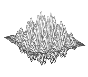
Figure 1. Characteristic features of the transport problems defined in Examples 5.1-5.4 (from left to right and top to bottom): (i) optimal transport plan given by a graph together with activated atoms and discrete support for $k=5$ in Example 5.1, (ii) optimal transport map $T=\nabla\Phi$ in Example 5.2 interpreted as a vector field, (iii) oscillating density $f$ in Example 5.3, (iv) piecewise affine optimal transport plan $T$ in Example 5.4.

5.2. Complexity considerations

A crucial quantity to determine the efficiency of our devised method is the growth of the cardinalities of the activated sets. In Table 1 we display for Examples 5.1-5.4 the corresponding numbers on different triangulations and for different cost functions. We observe that in all experiments the size of the activated sets grows essentially linearly in strong contrast to the quadratic growth of the theoretical number of unknowns of the corresponding discrete transport problem. A slight deviation of this behaviour occurs in Example 5.2 for $p=3$ where the increase of the active set size is larger than the expected factor 4. We note that we observed a reduction of the active set sizes by factors of approximately $2^{-d}$ compared to the sizes obtained with the algorithm from [OR15] for generic choices of parameters. Because of the very few required redefinitions of the active set, particularly for $p\geq 2$, we conclude that the optimality conditions provide a precise prediction of the supports even if only approximations of the multipliers are available, i.e., this property appears to be very robust with respect to perturbations of the multipliers.

$$\begin{array}[]{l||r|r|r|r}\hline\cr\hline\cr{\rm Ex.}~{}\ref{ex_1d}&k=7&k=8&k=9&k=10\\ \hline\cr M+N&258&514&1.026&2.050\\ MN&16.641&66.049&263.169&1.050.625\\ \hline\cr p=3/2&763\ (0)&1.531\ (0)&3.067\ (0)&6.139\ (0)\\ p=2&763\ (0)&1.531\ (0)&3.067\ (0)&6.139\ (0)\\ p=3&763\ (0)&1.539\ (0)&3.114\ (0)&6.442\ (0)\\[2.84526pt] \hline\cr\hline\cr{\rm Ex.}~{}\ref{ex_mae1}&k=3&k=4&k=5&k=6\\ \hline\cr M+N&506&1.906&7.394&29.122\\ MN&34.425&467.313&6.866.145&105.189.825\\ \hline\cr p=3/2&6.268\ (8)&27.846\ (1)&179.594\ (2)&745.713\ (1)\\ p=2&3.929\ (0)&15.729\ (0)&63.115\ (0)&252.951\ (0)\\ p=3&8.085\ (2)&56.703\ (2)&255.965\ (1)&1.847.207\ (2)\\[2.84526pt] \hline\cr\hline\cr{\rm Ex.}~{}\ref{ex_41}&k=3&k=4&k=5&k=6\\ \hline\cr M+N&162&578&2.178&8.450\\ MN&6.561&83.521&1.185.921&17.850.625\\ \hline\cr p=3/2&1.389\ (0)&20.787\ (7)&58.575\ (1)&183.465\ (1)\\ p=2&1.589\ (0)&5.755\ (0)&24.018\ (0)&103.100\ (0)\\ p=3&1.495\ (0)&6.319\ (0)&26.205\ (0)&106.857\ (0)\\[2.84526pt] \hline\cr\hline\cr{\rm Ex.}~{}\ref{ex_nonsmooth}&k=3&k=4&k=5&k=6\\ \hline\cr M+N&171&595&2.211&8.515\\ MN&7.290&88.434&1.21.858&18.125.250\\ \hline\cr p=3/2&1.346\ (0)&6.384\ (0)&24.135\ (0)&95.240\ (0)\\ p=2&1.654\ (0)&6.921\ (0)&29.106\ (0)&120.153\ (0)\\ p=3&1.274\ (0)&5.602\ (0)&21.353\ (0)&85.463\ (0)\\[2.84526pt] \hline\cr\hline\cr\end{array}$$

Table 1. Total number of nodes $M+N$, number of unknowns in the full optimization problem $MN$, and cardinalities of activated sets at optimality with number of tolerance increases in brackets in Examples 5.1-5.4 on triangulations with refinement level $k$ and different cost functions $c_{p}(x,y)$.

In Table 2 we display the total CPU time needed to solve the optimization problem on the $k$-th level. This includes the repeated activation of atoms, the repeated solution of the reduced linear programs, and the verification of the optimality conditions. We observe a superlinear growth of the numbers. These are dominated by the times needed to solve the linear programs whereas the (non-parallelized) verification of the optimality conditions was negligible in all tested situations.

$$\begin{array}[]{l||r|r|r|r}\hline\cr\hline\cr{\rm Ex.}~{}\ref{ex_1d}&k=7&k=8&k=9&k=10\\ \hline\cr p=3/2&0.0575&0.1357&0.4281&1.1840\\ p=2&0.0603&0.1288&0.3294&1.0257\\ p=3&0.0593&0.1345&0.3943&1.3115\\[2.84526pt] \hline\cr\hline\cr{\rm Ex.}~{}\ref{ex_mae1}&k=3&k=4&k=5&k=6\\ \hline\cr p=3/2&0.2063&0.8805&6.9296&49.5964\\ p=2&0.2187&0.5262&2.4734&21.1738\\ p=3&0.2584&1.6697&7.3599&97.7239\\[2.84526pt] \hline\cr\hline\cr{\rm Ex.}~{}\ref{ex_41}&k=3&k=4&k=5&k=6\\ \hline\cr p=3/2&0.1090&0.7655&1.5510&9.5078\\ p=2&0.1106&0.1718&0.7735&4.6622\\ p=3&0.1410&0.1886&0.8557&5.6919\\[2.84526pt] \hline\cr\hline\cr{\rm Ex.}~{}\ref{ex_nonsmooth}&k=3&k=4&k=5&k=6\\ \hline\cr p=3/2&0.1192&0.1777&0.8014&4.9880\\ p=2&0.1054&0.1766&0.6771&4.0459\\ p=3&0.1214&0.1700&0.7194&4.8851\\ \hline\cr\hline\cr\end{array}$$

Table 2. Total CPU time in seconds on $k$-th level in Examples 5.1-5.4 with different polynomial cost functions $c_{p}(x,y)$.

5.3. Experimental convergence rates

In Figures 2 and 3 we show for Examples 5.1 and 5.2 the error in the approximation of the optimal cost, i.e., the quantities

$$\delta_{h}=\big{|}\min_{\pi\geq 0}\widehat{I}[\pi]-\min_{\pi_{h}\geq 0}\widehat{I}_{h}[\pi_{h}]\big{|}$$

and the error in the approximation of the Lagrange multiplier $\phi$, i.e., the quantities

$$\varepsilon_{h}=\|\mathcal{I}_{X,h}\phi-\phi_{h}\|_{L^{\infty}(X)}.$$

If the exact optimal cost or the multiplier was not known, i.e., if $p\neq 2$, we used an extrapolated reference value or considered the difference $\mathcal{I}_{X,h}\phi_{h/2}-\phi_{h}$ to define $\delta_{h}$ and $\varepsilon_{h}$, respectively. We tested different polynomial costs and considered sequences of uniformly refined triangulations. Beause of the relation

$$h\sim(M+N)^{-1/d},$$

a quadratic convergence rate $\mathcal{O}(h^{2})$ corresponds to a slope $-2/d$ with respect to the total number of nodes $M+N$. Figure 2 confirms the estimate from Proposition 3.1 and additionally shows that the quadratic convergence rate is optimal. The experimental results also reveal that the employed quadratic tolerance in the verification of the optimality conditions in Algorithm 4.2 is sufficient to preserve the convergence rate of the linear program using the full set of atoms. Figure 3 indicates that quadratic convergence in $L^{\infty}(X)$ also holds for the approximation of the Lagrange multiplier $\phi$ provided this quantity is sufficiently regular. In particular, we observe here a slower convergence behaviour for $p=3/2$.

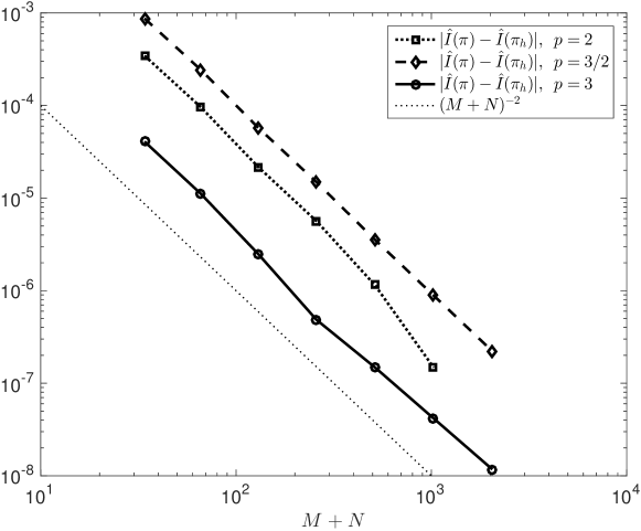
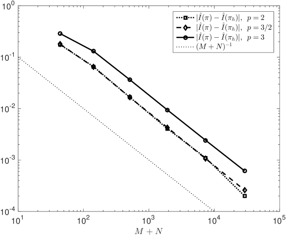
Figure 2. Experimental convergence of optimal costs in Examples 5.1 (left) and 5.2 (right) for different cost functions on sequences of uniformly refined triangulations.

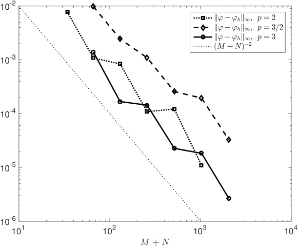
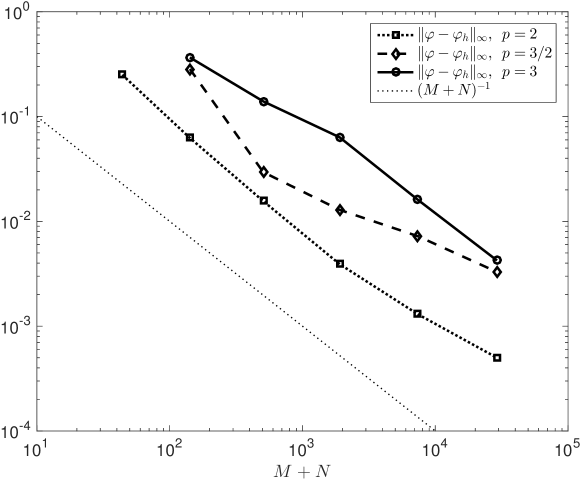
Figure 3. Experimental convergence rates of the discrete multiplier $\phi_{h}$ in Examples 5.1 (left) and 5.2 (right) for different cost functions on sequences of uniformly refined triangulations.

In [OR15] an approximately linear convergence rate in $L^{\infty}$ of the mulitpliers has been reported for Example 5.3 which is consistent with the piecewise constant approximation of densities of measures used in that article, cf. Remark 3.4. In particular, discrete duality yields that the Lagrange multipliers occurring in the discretized optimal transport problems are discretized in the same spaces. For our discretization using continuous, piecewise affine approximations we obtain a nearly quadratic experimental convergence rate in this example as well, as can be seen in Table 3 in which we also display the errors from [OR15].

$\varepsilon_{h}$	$h\sim 2^{-5}$	$h\sim 2^{-6}$	$h\sim 2^{-7}$	$h\sim 2^{-8}$	$h\sim 2^{-9}$
$P1$ (Alg. 4.2)	0.00781	0.00238	0.00086	–	–
$P0$ ([OR15])	0.00721	0.00892	0.00689	0.00241	0.00148

Table 3. Experimental errors $\varepsilon_{h}=\|\mathcal{I}_{h}\phi-\phi_{h}\|_{L^{\infty}(\Omega)}$ for discretizations using $P1$ and $P0$ approximations of densities in Example 5.3 with $p=2$.

Acknowledgments. SB acknowledges support by the DFG via the priority program Non-smooth and Complementarity-based Distributed Parameter Systems: Simulation and Hierarchical Optimization (SPP 1962).

References

- [BB00] Jean-David Benamou and Yann Brenier, A computational fluid mechanics solution to the Monge-Kantorovich mass transfer problem, Numer. Math. 84 (2000), no. 3, 375–393.
- [BC15] Jean-David Benamou and Guillaume Carlier, Augmented Lagrangian methods for transport optimization, mean field games and degenerate elliptic equations, J. Optim. Theory Appl. 167 (2015), no. 1, 1–26.
- [BFO14] Jean-David Benamou, Brittany D. Froese, and Adam M. Oberman, Numerical solution of the optimal transportation problem using the Monge-Ampère equation, J. Comput. Phys. 260 (2014), 107–126.
- [BS08] Susanne C. Brenner and L. Ridgway Scott, The mathematical theory of finite element methods, third ed., Texts in Applied Mathematics, vol. 15, Springer, New York, 2008.
- [BS17] Sören Bartels and Patrick Schön, Adaptive approximation of the monge-kantorovich problem via primal-dual gap estimates, Preprint, 2017.
- [CF17] Shibing Chen and Alessio Figalli, Partial regularity for optimal transport maps, J. Funct. Anal. 272 (2017), no. 11, 4588–4605.
- [DPF13] Guido De Philippis and Alessio Figalli, regularity for solutions of the Monge-Ampère equation, Invent. Math. 192 (2013), no. 1, 55–69.
- [Eva99] Lawrence C. Evans, Partial differential equations and Monge-Kantorovich mass transfer, Current developments in mathematics, 1997 (Cambridge, MA), Int. Press, Boston, MA, 1999, pp. 65–126.
- [GO16] Inc. Gurobi Optimization, Gurobi optimizer reference manual, 2016.
- [OR15] Adam M Oberman and Yuanlong Ruan, An efficient linear programming method for optimal transportation, arXiv preprint arXiv:1509.03668 (2015).
- [Rou97] Tomáš Roubíček, Relaxation in optimization theory and variational calculus, De Gruyter Series in Nonlinear Analysis and Applications, vol. 4, Walter de Gruyter & Co., Berlin, 1997.
- [RU00] Ludger Rüschendorf and Ludger Uckelmann, Numerical and analytical results for the transportation problem of Monge-Kantorovich, Metrika 51 (2000), no. 3, 245–258.
- [Sch16] Bernhard Schmitzer, A sparse multiscale algorithm for dense optimal transport, Journal of Mathematical Imaging and Vision 56 (2016), no. 2, 238–259.
- [Vil03] Cédric Villani, Topics in optimal transportation, no. 58, American Mathematical Soc., 2003.
- [Vil08] by same author, Optimal transport: old and new, vol. 338, Springer Science & Business Media, 2008.