Statistics of the relative velocity of particles in turbulent flows : monodisperse particles

Abstract

We use direct numerical simulations to calculate the joint probability density function of the relative distance $R$ and relative radial velocity component $V_{R}$ for a pair of heavy inertial particles suspended in homogeneous and isotropic turbulent flows. At small scales the distribution is scale invariant, with a scaling exponent that is related to the particle-particle correlation dimension in phase space, $D_{2}$. It was argued gustavsson2011distribution ; gustavsson2014relative that the scale invariant part of the distribution has two asymptotic regimes: ➀ $|V_{R}|\ll R$ where the distribution depends solely on $R$; and ➁ $|V_{R}|\gg R$ where the distribution is a function of $|V_{R}|$ alone. The probability distributions in these two regimes are matched along a straight line $|V_{R}|=z^{\ast}R$. Our simulations confirm that this is indeed correct. We further obtain $D_{2}$ and $z^{\ast}$ as a function of the Stokes number, St. The former depends non-monotonically on St with a minimum at about $\mbox{St}\approx 0.7$ and the latter has only a weak dependence on St.

I Introduction

Turbulent flows of gas with small heavy particles suspended in it is at the heart many natural phenomenon; typical examples are: (a) astrophysical dust is protoplanetary disks Arm10 , (b) small water droplets in clouds Pruppacher2010microphysics , and (c) aeolian processes (wind and sand) kok2012physics . In all of these cases, usually two crucial questions are studied: (a) whether the particles are homogeneously distributed in space or whether they can form clusters? and (b) what is the average collision velocities between the particles, which in turn determines the collision kernel – the number of collisions per-unit-time, per-unit-volume. Collisions between the particles play a crucial role in the dynamics of these systems, for example, some collisions between the water droplets in cloud may merge the droplets to form bigger droplets. A similar process of collision and consequent merging of dust grains plays a crucial role in formation of planetesimals (loosely held dust balls of size of the order of kilometers) in protoplanetary disks. Note that a complete knowledge of the collision kernel does not allow us to determine the probability of merging or coagulation which depends on one hand on the material properties of the colliding bodies and on the other hand on the probability distribution function of collision velocities. Clearly, a complete description of this problem is given by the joint probability distribution function (JPDF) of the separation ${\bm{R}}$ and relative velocity ${\bm{V}}$ of a pair of particles. The clustering of the particles in space and the collision kernel can be calculated from the zero-th and first moment of this JPDF respectively. In its full generality this is an extremely difficult problem to solve. Nevertheless, one can simplify the problem significantly and still preserve the essence of it. A commonly used model is that of heavy inertial particles, given by

$$\dot{{\bm{X}}} ={\bm{v}}\/,$$ (1a)

$$\dot{{\bm{v}}} =\frac{1}{\tau_{\rm p}}\left[{\bm{u}}({\bm{X}})-{\bm{v}}\right]\/.$$ (1b)

Here the dot denotes time differentiation, ${\bm{X}}$ and ${\bm{v}}$ are respectively the position and velocity of a particle, $\tau_{\rm p}$ is the characteristic relaxation time of the particle and ${\bm{u}}$ is the flow velocity that is determined by solving the Navier–Stokes equation with appropriate boundary conditions. Although the particles are approximated as points as far as the flow is concerned, they are assigned finite sizes to calculate the collision kernel.

The dynamics of heavy inertial particles in turbulence has been extensively studied, starting with the pioneering work by Saffman and Turner saf+tur55 . Since the turn of this century this problem has seen significant progress. For a detailed description we direct the reader to several recent reviews sha03 ; gra+wan13 ; tos+bod09 ; gus+meh16 ; pumir2016collisional . Here we give a very brief summary of the results that are directly relevant to this paper. The equations of motion for heavy inertial particles, Eq. (1), are clearly dissipative even if the flow velocity is incompressible. The stationary state of the system in phase-space is characterized by an attractor with a correlation dimensions $D_{2}<2d$ where $d$ is the dimension of space bec2003fractal . If $D_{2}<d$ then the particles also show clustering in real space bec04 with a spatial correlation dimension $d_{2}=D_{2}$. This gives rise to small-scale clustering which has been studied extensively using direct numerical simulations (see, e.g., bec2007heavy, ). There are two fundamentally distinct mechanisms that brings particles to close contact. One is driven by the flow gradients saf+tur55 , in which case the relative velocities of the particles goes to zero as the particles smoothly approach each other. The second mechanism allows particles to have non-negligible relative velocities at small distances falkovich2002acceleration ; wilkinson2006caustic . From Eq. (1) it follows that under quite general assumptions the gradient of the velocity of the HIPs, $\sigma_{ij}\equiv\delta v_{i}/\delta X_{j}$ develops singularities, caustics, in finite time wilkinson2006caustic . This implies that the relative velocity of two particles does not go to zero as their separation goes to zero but remains finite giving rise to a high collision kernel. Most of the theoretical, numerical, and experimental works have concentrated on calculating the clustering exponent $d_{2}$ and the collision kernel as a function of the Stokes number, $\mbox{St}=\tau_{\rm p}/t_{\rm\eta}$, where $t_{\rm\eta}$ is the characteristic time at the dissipative scales. The clustering exponent, $d_{2}$, can be obtained from the scaling exponent of the zero-th moment of this JPDF and the collision kernel is the first moment of the JPDF calculated at $\mid{\bm{R}}\mid=2a$ where $a$ is the radius of a particle. Our aim in this paper is to calculate this JPDF, particularly its scaling behavior from direct numerical simulations (DNS) of identical heavy inertial particles in forced, homogeneous, and isotropic, turbulent flows.

A significant amount of theoretical gustavsson2011distribution ; gustavsson2014relative , experimental de2010measurement ; saw+bew+bod+ray+bec14 , and numerical sun+col97 ; wang2000statistical ; hubbard2012turbulence ; pan2013turbulence ; per+jon15 work has gone into studying the joint probability distribution function, $\mathcal{P}({\bm{R}},{\bm{V}})$. Most of the numerical work has been limited to calculating $\mathcal{P}$ for few values of $R\equiv\mid{\bm{R}}\mid$. Some of the numerical works use either smooth random flows gustavsson2014relative ; gustavsson2011distribution or models of turbulence (e.g., a shell model, hubbard2012turbulence, ) instead of direct numerical simulations (DNS). The earliest DNS sun+col97 already pointed out that $\mathcal{P}$ for a fixed $R$ is not Gaussian, but possesses exponential tails. Some of the later studies wang2000statistical ; hubbard2012turbulence ; pan2013turbulence have confirmed the exponential tails and have demonstrated clear asymmetry between positive – a pair of particles moving away from each other – and negative – a pair of particles moving towards each other – side of $\mathcal{P}$. Ref. gustavsson2011distribution is the first paper to write down the Fokker-Planck equations satisfied by $\mathcal{P}$ by virtue of using a one-dimensional, random, smooth, white-in-time model for the flow velocity. The scaling behavior of $\mathcal{P}$ is obtained by solving the Fokker-Planck equation. Guided by this model, Ref gustavsson2014relative has argued that the JPDF, $\mathcal{P}$, possesses certain symmetries in quite general cases. A recent paper per+jon15 has used DNS to study the scaling behavior of the JPDF, $\mathcal{P}$, for several different values of $R$ and have confirmed some of the conclusions of Ref. gustavsson2014relative for $\mbox{St}\approx 1$. Our aim in this paper is to calculate $\mathcal{P}$, particularly its scaling behavior, from direct numerical simulations of identical heavy inertial particles in forced, homogeneous, and isotropic, turbulent flows.

The rest of this paper is organized as follows: in section II we briefly recapitulate the main theoretical results on scaling properties of $\mathcal{P}$, followed by section III where we describe in detail our direct numerical simulation; in section IV we show that our DNS indeed confirms these theoretical results, in particular, the symmetries and the scaling nature of $\mathcal{P}$; we conclude in section V.

II Theoretical Background

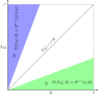
Figure 1: Schematic diagram of $R-|V_{R}|$ phase space. Light blue (➁) region of the phase space corresponds to the region where $|V_{R}|\gg R$. In this region the contribution due to caustics dominates and the joint probability density function $\mathcal{P}(R,|V_{R}|)$ becomes independent of $R$. The light green region (➀) corresponds to the region where $|V_{R}|\ll R$. In this region the relative velocity of the particles $V_{R}$ is a smooth function of their separation $R$, and $\mathcal{P}(R,|V_{R}|)$ is only a function of $R$. Two functions are matched along the line $|V_{R}|=z^{\ast}R$ to obtain the $\mathcal{P}(R,|V_{R}|)$.

We consider the flow to be forced at large length scales, statistically stationary, homogeneous and isotropic. The model of heavy inertial particles, Eq. (1), is applicable if the size of the particles are smaller than the smallest energy carrying length scale of the turbulence – the Kolmogorov scale, $\eta$. The characteristic velocity at the length scale is $u_{\rm\eta}$ such that the scale-dependent Reynolds number of the Kolmogorov scale is $\mbox{Re}_{\eta}=u_{\rm\eta}\eta/\nu=1$ where $\nu$ is the kinematic viscosity of the fluid. As we are primarily interested in particle collisions, we are interested in relative velocities of particles at small separations – smaller than $\eta$. In what follows we use $\eta$ and $u_{\rm\eta}$ as our characteristic scales of length and velocity respectively.

As mentioned in the introduction two fundamentally distinct mechanisms may bring particles into contact at small separations in turbulent aerosols. In the first case saf+tur55 the particles are brought together by the turbulent flow velocity; they spend a long time together, smoothly approaching each other towards small spatial separations. Their phase-space separation approaches zero as their relative distance goes to zero. The second possibility falkovich2002acceleration ; wilkinson2006caustic ; gustavsson2014relative is that the particles detach from the flow, allowing caustics to form, leading to a multi-valued particle velocity field. If the detachment is large enough compared to the distance between two particles they may move towards each other close to ballistically. The latter effect give rise to particle collisions with large relative velocities – the phase-space separation remains finite as the distance approaches zero. These observations were used in Refs. gustavsson2011distribution ; gustavsson2014relative to calculate the asymptotic behavior of the joint probability distribution of separations and relative velocities, $\mathcal{P}({\bm{R}},{\bm{V}})$, in a smooth, homogeneous and isotropic flow.

The radial projection $V_{R}=({\bm{V}}\cdot{\bm{R}})/R$ of ${\bm{V}}$ plays a crucial role in the collision between the particles. As two particles detach from the relative flow velocity at large separations, their ballistic motion will bring them into contact at small separations if their tangential velocity is close to zero, i.e. if ${\bm{V}}\approx V_{R}{\bm{R}}/R$ and if $V_{R}$ is negative. In spherical coordinates, in $d$ dimensions, we write the joint distribution of $R$ and $|V_{R}|$ as

$$\mathcal{P}(R,|V_{R}|)=R^{d-1}f(R,|V_{R}|)\,,$$ (2)

where the factor of $R^{d-1}$ comes from the spatial volume element. This volume element corrects for the probability of having a small tangential velocity, and we can think of $f(R,|V_{R}|)$ to be the probability to have velocity $|V_{R}|$ at distance $R$ in the two-dimensional system formed by $R$ and $|V_{R}|$. We summarize the theoretical predictions gustavsson2014relative of $\mathcal{P}(R,|V_{R}|)$ below.

1. The distribution $\mathcal{P}$, reduces to two asymptotic forms

   $$P(R ,|V_{R}|)\sim$$ (3)

   $$R^{d-1}\left\{\begin{array}[]{lll}{{f_{1}}}(R,|V_{R}|)&\mbox{for }|V_{R}|\leq\Upsilon(R)&\mbox{\raisebox{-1.42271pt}{\large\char 192}}\cr{{f_{1}}}(\Upsilon^{-1}(|V_{R}|),|V_{R}|)&\mbox{for }|V_{R}|>\Upsilon(R)&\mbox{\raisebox{-1.42271pt}{\large\char 193}}\cr\end{array}\right.\,.$$ (6)

   These two asymptotic limits are illustrated as region ➁ and region ➀ respectively in Fig. (1), and are matched along an curve $|V_{R}|=\Upsilon(R)$ [The curve $\Upsilon(R)=z^{\ast}R$ is shown in Fig. (1)].

2. For relative distances smaller than the dissipation scale, i.e., $R<1$, the flow velocity can be approximated by a smooth flow, in which case the matching curve is found to be

   $$\Upsilon(R)=z^{\ast}R\quad\mbox{for}\quad R<1\/,$$ (7)

   where $z^{\ast}$ is a constant.

3. The scaling function in the dissipation range is,

   $${{f_{1}}}(R,|V_{R}|)\sim R^{D_{2}-d-1}\quad\mbox{for}\quad R<1\,,$$ (8)

   where $D_{2}$ is the correlation dimension of the attractor of the long-time stationary state of the particles in phase space.

We shall call the predictions 1 and 2 together the “asymptotic mirror symmetry” of $\mathcal{P}$ in the dissipation range. This is because the distribution in region ➀ is effectively mirrored in the curve $|V_{R}|=z^{\ast}R$, giving the distribution in region ➁. In this paper we show, from direct numerical simulations, that all the above predictions hold.

III Direct Numerical Simulations

The flow velocity ${\bm{u}}$ is obtained by direct numerical simulation (DNS) of the Navier–Stokes equation,

$$\partial_{t}\rho +\nabla\cdot(\rho{\bm{u}})=0\/,$$ (9a)

$$\rho D_{t}{\bm{u}} =-\nabla p+\mu\nabla\cdot{\bm{S}}+{\bm{f}}\/,$$ (9b)

under isothermal conditions, with an external force. Here $D_{t}\equiv\partial_{t}+{\bm{u}}\cdot\nabla$ is the advective derivative, $p$, and $\rho$ are respectively the velocity, pressure, and density of the flow, $\mu$ is the dynamic viscosity, and ${\bm{S}}$ is a second-rank tensor with components $S_{kj}\equiv\partial_{k}u_{j}+\partial_{j}u_{k}-\delta_{jk}(2/3)\partial_{k}u_{k}$. The simulations are performed in a three-dimensional periodic box with sides $L_{\rm x}=L_{\rm y}=L_{\rm z}=2\pi$. In addition we use the ideal gas equation of state with a constant speed of sound $c_{\rm s}=1$.

We use the Pencil-Code pencil-code , which uses a sixth-order finite-difference scheme for space derivatives and a third-order Williamson-Runge-Kutta wil80 scheme for time derivatives. The external force ${\bm{f}}$ is a white-in-time stochastic process that is integrated by using the Euler–Marayuma scheme (hig01, ). The same setup have been used in studies of scaling and intermittency in fluid and magnetohydrodynamic turbulence dob+hau+you+bra03 ; hau+bra+dob03 ; hau+bra04 . We introduce the particles into the DNS after the flow has reached statistically stationary state. Then we simultaneously solve the equations of the flow, Eq. (9), and the heavy inertial particles, Eq. (1). To solve for the particles in the flow we have to interpolate the flow velocity to typically off-grid positions of the particles. We use a tri-linear method for interpolation.

The flow attains a statistically stationary state when the average energy dissipation by viscous forces is balanced by the average energy injection by the external force ${\bm{f}}$ which is concentrated on a shell of wavenumber with radius $k_{\rm f}$ in Fourier space B01 . We define the Reynolds number by $\mbox{Re}\equiv u_{\rm rms}/(\nu k_{\rm f})$, where $u_{\rm rms}$ is the root-mean-square velocity of the flow averaged over the whole domain and the kinematic viscosity $\nu=\mu/\langle\rho\rangle$ where the symbol $\langle\cdot\rangle$ denotes spatial and temporal averaging over the statistically stationary state of the flow. The mean energy dissipation rate is $\varepsilon\equiv 2\nu\langle\omega^{2}\rangle$, where $\omega\equiv{\bm{\nabla}}\times{\bm{u}}$ is the vorticity. The Kolmogorov scale or the dissipation length scale is given by $\eta\equiv(\nu^{3}/\varepsilon)^{1/4}$, the characteristic time scale of dissipation is given by $t_{\rm\eta}=\sqrt{\nu/\varepsilon}$ and $u_{\rm\eta}\equiv\eta/t_{\rm\eta}$ is the characteristic velocity scale at the dissipation length scale. In our simulations, unless otherwise stated, we use $\eta$, $t_{\rm\eta}$, and $u_{\rm\eta}$ to non-dimensionalize length, time, and velocity respectively. The large eddy turnover time is given by $T_{\rm eddy}\equiv 1/k_{\rm f}u_{\rm rms}$. We define the Stokes number $\mbox{St}\equiv\tau_{\rm p}/t_{\rm\eta}$.

The amplitude of the external force is chosen such that the Mach number, $\mbox{Ma}\equiv u_{\rm rms}/c_{\rm s}$ is always less than $0.1$, i.e., the flow is weakly compressible. If on one hand we consider application of our DNS to understand rain-formation in Earth’s atmosphere it would be appropriate to consider an incompressible flow. We have checked that the weak compressibility in our DNS does not have any significant effect in the following manner: (a) The probability density of ${\bm{\nabla}}\cdot{\bm{u}}$ along particle trajectories is found to be a Gaussian highly peaked at zero, see Appendix A, Fig. (8). (b) We parametrise the compressibility by calculating the dimensionless number $\mathfrak{p}=\langle\mid{\bm{\nabla}}\cdot{\bm{u}}\mid^{2}\rangle/\langle\mid{\bm{\nabla}}\times{\bm{u}}\mid^{2}\rangle=8.6\times 10^{-3}$. Following Ref. gus+meh16 we estimate that $\mathfrak{p}=8.6\times 10^{-3}$ implies that the compressibility of the flow may have significant effect only on particles with $\mbox{St}\lesssim 0.11$ whereas the smallest value of St used in our simulations is $0.17$. (c) And finally we calculate the correlation dimension, $d_{\rm 2}$, of the cluster formed by the particles to find that our results agree with those obtained in incompressible flows bec2007heavy . On the other hand, if we consider possible application of our work to astrophysical problems, e.g., to protoplanetary disks pan2013turbulence then indeed the weakly compressible simulations are the appropriate model.

Table 1: Table of parameters for our DNS runs with $N^{3}$ collocation points: $\nu$ the coefficient of kinematic viscosity, $N_{\rm p}$ is the number of particles, $\epsilon$ in the mean rate of energy dissipation, $\eta\equiv(\nu^{3}/\epsilon)^{1/4}$ and $t_{\rm\eta}=\sqrt{(\nu/\epsilon)}$ are the dissipation length and time scales, respectively, Re is the Reynolds number based on forcing length scale, and $T_{\rm eddy}$ is large eddy turn-over time scale of the flow.

Run	$N$	$\nu$	$N_{\rm p}$	Re	$\varepsilon$	$\eta$	$t_{\rm\eta}$	$T_{\rm eddy}$
R1	$256$	$1.0\times 10^{-3}$	$10^{7}$	$41$	$3.02\times 10^{-3}$	$2.4\times 10^{-2}$	$0.56$	$0.93$
R2	$512$	$5.0\times 10^{-4}$	$10^{7}$	$89$	$3.25\times 10^{-3}$	$1.4\times 10^{-2}$	$0.39$	$0.86$

IV Results

To calculate the JPDF we need to look at all pairs of particles within a separation of $\eta$. Naively speaking this process scales quadratically with the number of particles, $N_{\rm p}^{2}$, but using the standard technique of constructing linked-lists – commonly used in molecular dynamics simulations (see, e.g., All+Til89, , Chapter 5), we can reduce number of computations to be proportional to $N_{\rm p}$. The same technique has been used before in Refs. sun+col97 ; per+jon15 .

IV.1 Correlation dimensions

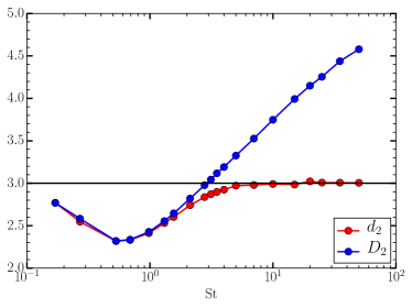
Figure 2: Phase-space correlation dimension ${\rm D}_{2}$ and real-space correlation dimension ${\rm d}_{2}$ as functions of St. Black dashed curve shows the data from Ref bec2007heavy .

To calculate the phase-space correlation dimension we evaluate the $\mathcal{P}(w)$ which is the probability distribution function (PDF) of $w$, where $w^{2}=\mid{\bm{R}}\mid^{2}+\mid{\bm{V}}\mid^{2}$. We calculate $D_{2}$ by the scaling behavior:

$$\mathcal{P}(w)\sim w^{D_{2}-1}\quad{\rm as}\quad w\to 0$$ (10)

In Fig. (2) we plot $D_{2}$ as a function of St for the run R2. In the range of St we have calculated, $D_{2}$ is non-monotonic function of St with a minimum near $\mbox{St}\approx 0.7$ and does not change significantly as a function of Re. Next we calculate the real-space radial distribution function (RDF), $g(R)$, which is the PDF of $R$. At small $R$, the RDF show scaling behavior:

$$g(R)\sim R^{d_{2}-1}\quad{\rm as}\quad R\to 0$$ (11)

The small scale clustering of HIPs in real space is parametrised by $d_{2}$ which is plotted for the run R2. The values of $d_{\rm 2}$ we obtain is equal to (within error bars) the earlier value of $d_{\rm 2}$ obtained in Ref bec2007heavy . Note that a crucial component of the theory described in Ref. gustavsson2014relative is not $d_{\rm 2}$ but $D_{2}$ – the phase-space correlation dimension. Under fairly general conditions, it can be shown that bec04 if the particles cluster on a fractal set in phase-space with correlation dimension $D_{2}$ then their real space correlation dimension $d_{\rm 2}={\rm min}(D_{2},d)$ where $d=3$ is the dimension of space. To the best of our knowledge, $D_{2}$ has never been calculated before for HIPs in turbulent flows, although they have been calculated for smooth random flows.

IV.2 Joint PDFs of $R$ and $|V_{R}|$

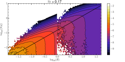
Figure 3: (color online) Contour plots of joint PDFs, $\mathcal{P}(R,|V_{R}|)$, divided by $R^{2}$, for four representative values of St plotted in logarithmic scales. The joint PDF for $R<1$ and $R>1$ are calculated separately and then patched together.

Before we present our results on the JPDF, $\mathcal{P}(R,|V_{R}|)$ let us note that the scaling theory of Ref. gustavsson2011distribution does not distinguish between the positive and negative components of $V_{R}$, i.e., it does not distinguish between two particles approaching each other and moving away from each other. In the same spirit, unless otherwise stated, we present below the numerical data on $\mathcal{P}(R,|V_{R}|)$.

We plot in Fig. (3) contour plots of the joint PDF, $\mathcal{P}(R,|V_{R}|)$ for four different values of St. Let us first consider the top figures in the left column, $\mbox{St}=0.17$. Looking at the region ➀ of these figures we find that the contour lines are vertical, i.e., in region ➀ $\mathcal{P}(R,|V_{R}|)$ is a function of $R$ alone. But we have practically no data in the region corresponding to ➁ in this figure. This is expected because in region ➁ the contribution due to caustics dominate $\mathcal{P}$, but caustics are exponentially suppressed with St for small values of St wilkinson2006caustic . Note also that for a fixed but small St we should always be able to find the contribution from the caustics if we can probe small enough $R$. But at small St there are few particle pairs whose separation is very small. This is because the real-space clustering exponent $d_{2}$ is quite close to $d=3$ for small $R$. These two factors explain why we have difficulty observing the contribution from the caustics at small St. Looking at the higher values of St in Fig. (3), we indeed find that the contour lines of $\mathcal{P}$ in region ➁ become horizontal, i.e., $\mathcal{P}(R,|V_{R}|)$ becomes a function of $|V_{R}|$ alone. We estimate the matching scale $z^{\ast}$ from left column of Fig. (3) by fitting a line through the points where contours change from vertical to horizontal. This line is the matching curve $\Upsilon(R)$. It is clear from the figure that this matching line continues beyond its theoretically predicted regime, $R<1$ to at least up to $R\gtrsim 10$ for all the St values we have studied.

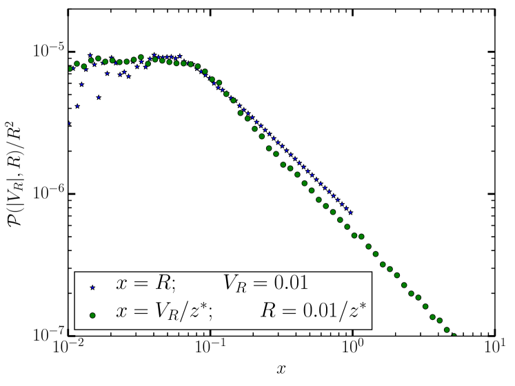
Figure 4: (color online) The joint PDF, $\mathcal{P}$, for $\mbox{St}=3.13$, as a function of $R$ for a fixed $|V_{R}|$ plotted with symbols $\ast$. The same PDF plotted along a vertical line, which is the mirror image of the horizontal line about the line $\Upsilon(R)=z^{\ast}R$ is plotted with the symbol $\cdot$.

Next, to test the asymptotic mirror symmetry of $\mathcal{P}$, we plot in Fig. (4), $\mathcal{P}$ along a horizontal line as a function of $R$, for $R<1$, for a small value of $|V_{R}|$. Then we reflect this line about the matching curve $\Upsilon(R)$ to obtain a vertical line and then plot $\mathcal{P}$ along this vertical line in the same plot, Fig. (4). Thus we confirm the asymptotic mirror symmetry of $\mathcal{P}$.

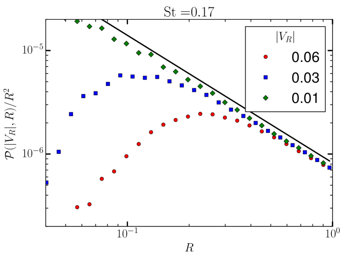
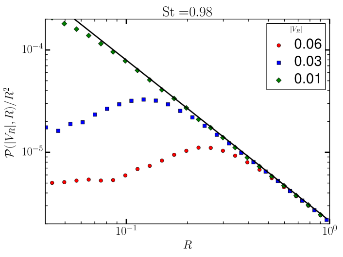
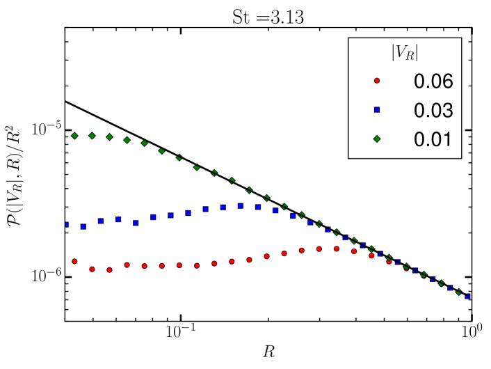
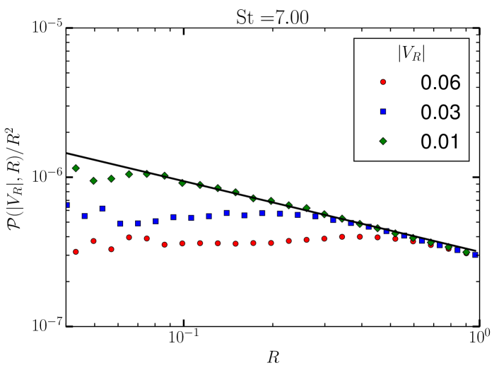
Figure 5: (color online) log-log plots of $\mathcal{P}(R,|V_{R}|)/R^{2}$ versus $R$, for four representative values of St. For each value of St we plot the curves for three fixed values of $|V_{R}|$. The solid black line in each plot has slope $D_{2}-4$, where $D_{2}$ depends on St as shown in Fig. (2)

Continuing with our quantitative tests we plot in the four panels of Fig. (5), $\mathcal{P}(R,|V_{R}|)/R^{2}$ as a function of $R$ for four different values of St. On each panel we plot three different values of $|V_{R}|$. According to the theoretical prediction, Eq. (3), we expect to find scaling with an exponent of $D_{2}-4$ which is indeed confirmed.

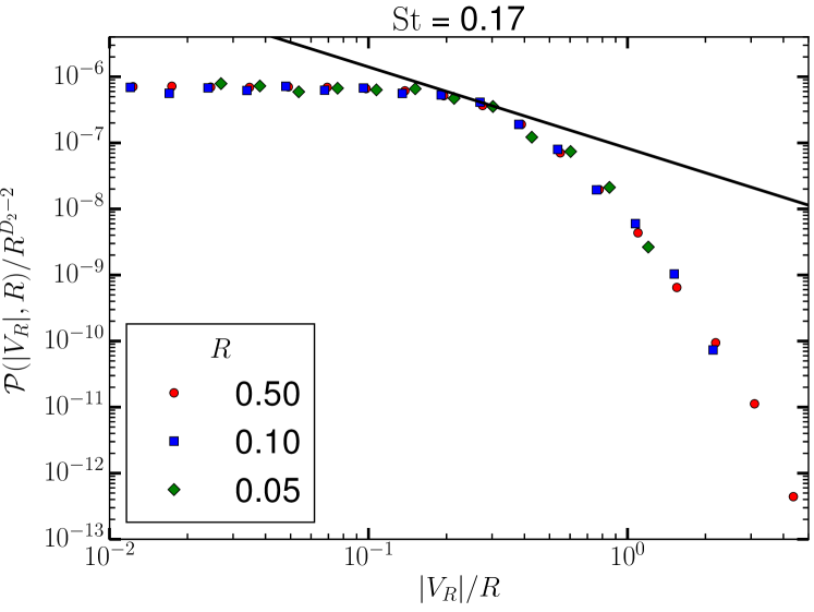
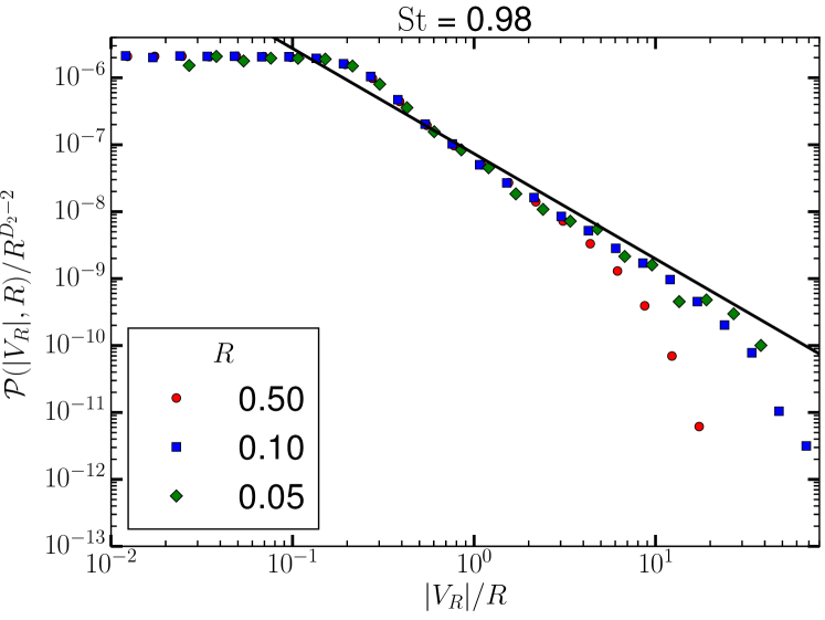
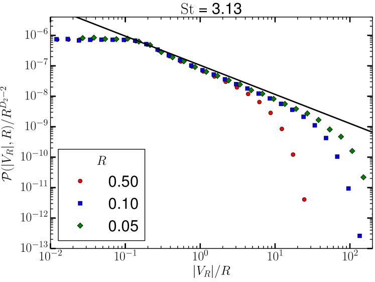
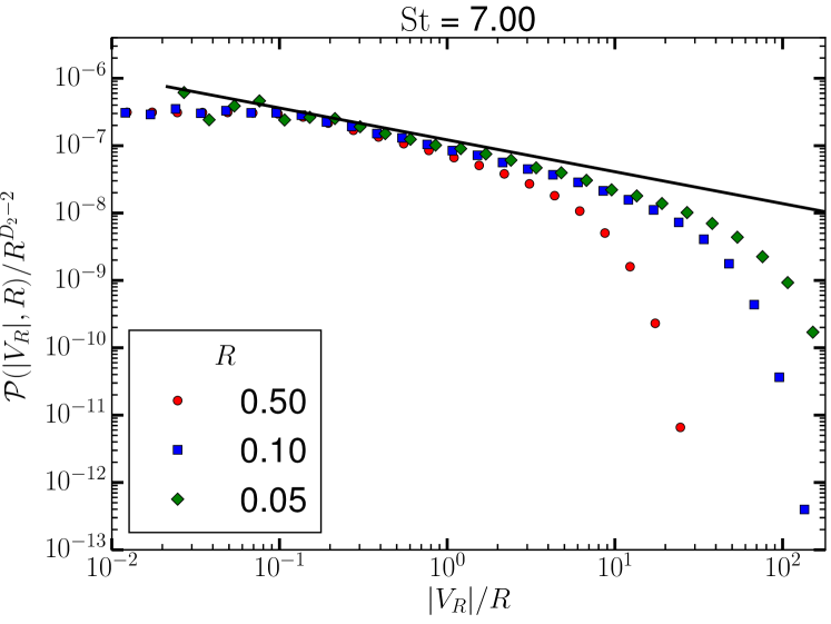
Figure 6: (color online) log-log plots of $\rho(V_{R},R)/R^{D_{2}-4}$ versus $V_{R}/R$, for four representative values of St. For each value of St we plot the curves for three different values of $R$. The solid line in each plot has slope $D_{2}-4$, where $D_{2}$ depends on St.

Next let us consider the PDF of $|V_{R}|$ for a fixed $R$, $P_{\rm R}(|V_{R}|)=\mathcal{P}(R,|V_{R}|)$. The scaling prediction for $\mathcal{P}$ as given in Eq. (8) would imply that $\mathcal{P}(R,|V_{R}|)\sim|V_{R}|^{D_{2}-d-1}\sim|V_{R}|^{D_{2}-4}$ for a fixed $R$. Looking back at the contour plot of $\mathcal{P}$ in Fig. (3) for, e.g., $\mbox{St}=0.69$ we realize that $P_{\rm R}$ can be obtained by taking a vertical cut through this figure. As the contour is almost horizontal until it reaches the matching line, we expect $P_{\rm R}$ to be independent of $|V_{R}|$, for $|V_{R}|<z^{\ast}R$ and proportional to $R^{D_{2}-2}$ until it reaches the upper cutoff at $|V_{R}|\approx z^{\ast}$. Hence we expect that if we plot $P_{\rm R}(|V_{R}|)/R^{D_{2}-2}$ versus $(|V_{R}|/R)$ for different values of $R$ we would obtain a data collapse to an universal function with a scaling exponent of $D_{2}-4$. This we do for four different values of St in four panels of Fig. (6). On each panel we plot the data for three different values of $R<1$. For the smallest St, $\mbox{St}=0.17$, we do see a collapse of the data but no scaling behavior. This happens because the scaling appears due to the contribution from the caustics and at small St we have not been able to probe small enough distances $R$ to see scaling. Indeed the scaling behavior appears for the next two values of St, $\mbox{St}=0.98$ and $3.13$ with the values of $D_{2}$ obtained from Fig. (2). At large $|V_{R}|$ we find departure from the data collapse. This is what one would expect because the cutoff to the scaling behavior is set by $z^{\ast}$ which is independent of $R$.

Next we consider the scale $z^{\ast}$. The scaling theory has no way of determining this, we calculate this as the best fit to our data and plot it as a function of St in Appendix B, Fig. (9). We find that $z^{\ast}$ varies very little – within a factor of two – as St changes by two orders of magnitudes. In principle $z^{\ast}$ can also depend on Re, within the range of Re studied in our simulations, it does not have any significant dependence on Re.

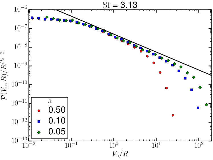
Figure 7: (color online) log-log plot of $\mathcal{P}(R,V_{\rm n})/R^{D_{2}-2}$ versus $V_{\rm n}/R$, for $\mbox{St}=3.13$ and three values of $R$. Here $V_{\rm n}$ is the negative relative longitudinal velocity between two particles separated by a distance $R$. The solid black line has slope $D_{2}-4$. Comparing this figure with Fig. (6) we find that the distributions of $V_{\rm n}$ and $|V_{R}|$ has the same scaling behavior.

Note finally that so far we have presented all our numerical results for the absolute value of $V_{R}$ ignoring its sign. But the sign of $V_{R}$ is crucial as it sets the collision kernel. We have checked that the statistics of negative side of $V_{R}$, defined by $V_{\rm n}$, follows exactly the same scaling behavior as that of $|V_{R}|$. To demonstrate this we plot in Fig. (7) the scaling collapse of the joint PDF of $R$ and $V_{\rm n}$ for $\mbox{St}=3.13$. Comparing this figure with Fig. (6) we find that the distributions of $V_{\rm n}$ and $|V_{R}|$ has the same scaling behavior.

V Conclusions

To summarize, the joint PDF, $\mathcal{P}$, gives a complete description of the statistics of relative velocities and distances of a pair of heavy inertial particles in homogeneous and turbulent flows. Quantities of more practical interest, for example, the spatial clustering and the collision kernel follows from this joint PDF. Our simulations confirms the theoretically predicted asymptotic mirror symmetry of $\mathcal{P}$ about a matching line $\Upsilon(R)=z^{\ast}R$. Furthermore, our DNS confirms the scaling behavior predicted in Ref. gustavsson2011distribution . The scale $z^{\ast}$ sets the cutoff to the scaling behavior of PDF of $|V_{R}|$, hence it sets the maximum possible relative velocities; as we have non-dimensionalized all velocities using $u_{\rm\eta}$. This implies that the maximum collision speed of heavy inertial particles in turbulent flows is of the order of $z^{\ast}u_{\rm\eta}$. In our DNS we find that $z^{\ast}$ depends very weakly on St in contradiction to the results of white-noise model in Ref gustavsson2011distribution , who found $z^{\ast}\sim\mbox{St}$.

To the best of our knowledge, the joint PDF and its scaling properties have never been calculated from DNS of homogeneous and isotropic turbulent flows, although it has been calculated numerically for two-dimensional random smooth flows and analytically for a one-dimensional white-noise model gustavsson2011distribution . Other than Ref. gustavsson2011distribution , Ref. pan2013turbulence has presented theoretical arguments and DNS results on PDF of $|V_{R}|$ for a given $R$. However Ref. pan2013turbulence did not elucidate the scaling nature of the PDF instead concentrated on the large-$|V_{R}|$ cutoff of the PDF. Ref. per+jon15 have obtained PDF of $V_{R}$ for several values of $R$ from DNS and had confirmed the scaling behavior for $\mbox{St}\approx 1$, but they did not study the asymptotic mirror symmetry. There are also limited experimental data de2010measurement ; saw+bew+bod+ray+bec14 available for $V_{R}$ but most of it is limited to $R\simeq\eta$ hence is not sufficient to study the scaling behavior as we do.

VI Acknowledgment

This work is supported by the grant Bottlenecks for particle growth in turbulent aerosols from the Knut and Alice Wallenberg Foundation (Dnr. KAW 2014.0048). The computations were performed on resources provided by the Swedish National Infrastructure for Computing (SNIC) at PDC.

Appendix A ${\bm{\nabla}}\cdot{\bm{u}}$ along the particle tracks

In our simulations the flow velocity field ${\bm{u}}$ is weakly compressible. To test the effect of this weak compressibility on the dynamics of heavy inertial particles, we calculate ${\bm{\nabla}}\cdot{\bm{u}}$ at the position of particles. This is done by first calculating ${\bm{\nabla}}\cdot{\bm{u}}$ at the grid points and then interpolating it to the positions of particles. We plot the PDFs of ${\bm{\nabla}}\cdot{\bm{u}}$ along the trajectories of particles having three different values of St in Fig. (8). We non-dimensionalize ${\bm{\nabla}}\cdot{\bm{u}}$ by the inverse of $t_{\rm\eta}$, which gives an idea of shear at the Kolmogorov scale $\eta$. In Fig. (8), we see that the PDFs are Gaussian with a high peak at zero and have a small width compared to $1/t_{\rm\eta}$. We also observe that these distributions does not depend on the value of St. These observations suggest that ${\bm{\nabla}}\cdot{\bm{u}}$ does not attain very high values along the trajectories of particles and effects of compressibility are weak.

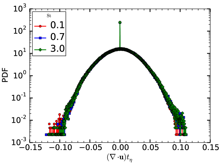
Figure 8: (color online) PDFs of $\nabla\cdot{\bm{u}}$ calculated along the trajectories of particles for three values of St, from the run R2

Appendix B Matching scale $z^{\ast}$

We show in Fig. (3) that the joint PDFs in regions ➀  and ➁  can be matched along a straight line $|V_{R}|=z^{\ast}R$, for $R<1$. We find the matching scale $z^{\ast}$ by fitting a straight line through the points where contour lines in Fig. (3) turns from vertical to horizontal. We show the plot of $z^{\ast}$ as a function of St if Fig. (9). We find that $z^{\ast}$ weakly depends on St. Its value remains close to $10^{-1}$. Values of $z^{\ast}$ for small values of St are not reliable because for small St [c.f. Fig. (3) (a)] we do not see the asymptotic regime in region ➁.

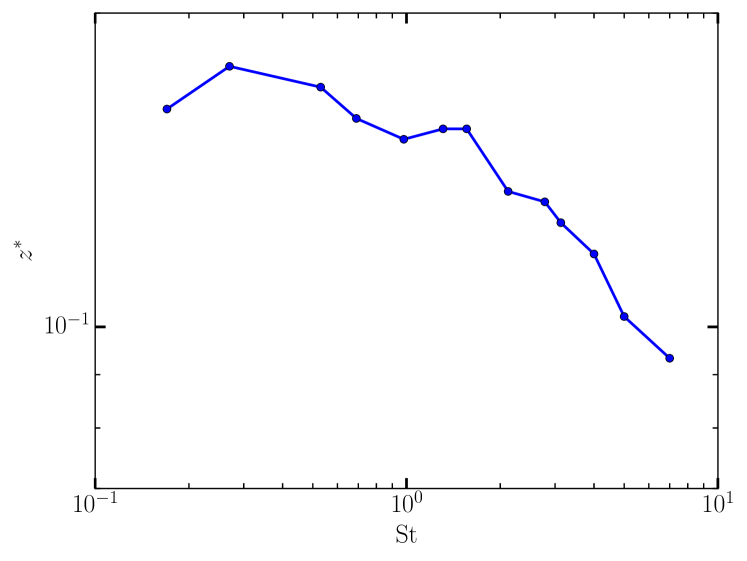
Figure 9: (color online) Matching scale $z^{\ast}$ as a function of St from the run R2

References

- (1) K. Gustavsson and B. Mehlig, Physical Review E 84, 045304 (2011).
- (2) K. Gustavsson and B. Mehlig, Journal of Turbulence 15, 34 (2014).
- (3) P. J. Armitage, Astrophysics of Planet Formation (Cambridge University Press, Cambridge, UK, 2010).
- (4) H. Pruppacher and J. Klett, Microphysics of Clouds and Precipitation (Springer Science & Business Media, ADDRESS, 2010), Vol. 18.
- (5) J. F. Kok, E. J. Parteli, T. I. Michaels, and D. B. Karam, Reports on Progress in Physics 75, 106901 (2012).
- (6) P. Saffman and J. Turner, Journal of Fluid Mechanics 1, 16 (1956).
- (7) R. A. Shaw, Annual Review of Fluid Mechanics 35, 183 (2003).
- (8) W. W. Grabowski and L.-P. Wang, Annual Review of Fluid Mechanics 45, 293 (2013).
- (9) F. Toschi and E. Bodenschatz, Ann. Rev. Fluid Mech. 41, 375 (2009).
- (10) K. Gustavsson and B. Mehlig, Advances in Physics 65, 1 (2016).
- (11) A. Pumir and M. Wilkinson, Annual Review of Condensed Matter Physics 7, 141 (2016).
- (12) J. Bec, Physics of fluids 15, L81 (2003).
- (13) J. Bec, Journal of Fluid Mechanics 528, 255 (2005).
- (14) J. Bec et al., Physical review letters 98, 084502 (2007).
- (15) G. Falkovich, A. Fouxon, and M. Stepanov, Nature 419, 151 (2002).
- (16) M. Wilkinson, B. Mehlig, and V. Bezuglyy, Physical review letters 97, 048501 (2006).
- (17) J. De Jong et al., International Journal of Multiphase Flow 36, 324 (2010).
- (18) E.-W. Saw et al., Physics of Fluids (1994-present) 26, 111702 (2014).
- (19) S. Sundaram and L. R. Collins, Journal of Fluid Mechanics 335, 109 (1997).
- (20) L.-P. Wang, A. S. Wexler, and Y. Zhou, Journal of Fluid Mechanics 415, 117 (2000).
- (21) A. Hubbard, Monthly Notices of the Royal Astronomical Society 426, 784 (2012).
- (22) L. Pan and P. Padoan, The Astrophysical Journal 776, 12 (2013).
- (23) V. E. Perrin and H. J. Jonker, Physical Review E 92, 043022 (2015).
- (24) A. Brandenburg and W. Dobler, Computer Physics Communications 147, 471 (2002).
- (25) J. Williamson, Journal of Computational Physics 35, 48 (1980).
- (26) D. Higham, SIAM Review 43, 525 (2001).
- (27) W. Dobler, N. E. L. Haugen, T. A. Yousef, and A. Brandenburg, Physical Review E 68, 026304 (2003).
- (28) N. E. L. Haugen, A. Brandenburg, and W. Dobler, The Astrophysical Journal Letters 597, L141 (2003).
- (29) N. E. L. Haugen and A. Brandenburg, Phys. Rev. E 70, 026405 (2004).
- (30) A. Brandenburg, ApJ550, 824 (2001).
- (31) M. P. Allen and D. J. Tildesley, Computer simulation of liquids (Oxford university press, ADDRESS, 1989).