Abstract. Meirowitz [17] showed existence of continuous behavioural function equilibria for Bayesian games with non-finite type and action spaces. A key condition for the proof of the existence result is equi-continuity of behavioural functions which, according to Meirowitz [17, page 215], is likely to fail or difficult to verify. In this paper, we advance the research by presenting some verifiable conditions for the required equi-continuity, namely some growth conditions of the expected utility functions of each player at equilibria. In the case when the growth is of second order, we demonstrate that the condition is guaranteed by strong concavity of the utility function. Moreover, by using recent research on polynomial decision rules and optimal discretization approaches in stochastic and robust optimization, we propose some approximation schemes for the Bayesian equilibrium problem: first, by restricting the behavioural functions to polynomial functions of certain order over the space of types, we demonstrate that solving a Bayesian polynomial behavioural function equilibrium is down to solving a finite dimensional stochastic equilibrium problem; second, we apply the optimal quantization method due to Pflug and Pichler [18] to develop an effective discretization scheme for solving the latter. Error bounds are derived for the respective approximation schemes under moderate conditions and both academic examples and numerical results are presented to explain the Bayesian equilibrium problem and their approximation schemes.

Key words. Bayesian game, behavioural function equilibrium, equi-continuity, polynomial decision rules, rent-seeking contest

1 Introduction

Over the past few years, there has been an increasing attention to Nash games with private information. A common assumption in such games is that the prior distribution of the types of all players is known in public, each player has complete information of its own type which determines its utility function but is unaware of its rival’s type. Based on the prior information, each player chooses a response function which is also known as behavioural function defined over its type space under Nash conjecture and an equilibrium arising from this kind of game is known as Bayesian Nash equilibrium, see Hansanyi [14] for a comprehensive original discussion of the Bayesian games where private information might also include other aspects of a player’s payoff function.

Meirowitz [17] considered a Bayesian game where each player chooses its behavioural function based on maximization of its expected utility with the expectation being taken w.r.t. its rival’s distribution of types conditional on the selection of its own type. Under some conditions, he established existence of equilibria for the Bayesian game using Schauder’s fixed point theorem. One of the main conditions that Meirowitz used for the existence result is equi-continuity of the behavioural functions which is elicited to ensure that the space of behavioural functions is closed and the operator mapping the set of behaviour functions to itself is compact. Meirowitz commented that the equi-continuity condition is likely to fail or difficult to verify in practical applications. Athey [2] considered a class of Bayesian games where the types are drawn from an atomless joint probability distribution and each player’s utility function has so-called single crossing property which means whenever each opponent uses a nondecreasing strategy in the sense that higher types choose higher actions, a player’s best response strategy is also nondecreasing. Under these circumstances, she demonstrated existence of equilibria in every finite-action game with each player’s behavioural function being nondecreasing and step-like. Moreover, when the space of actions is continuous, she showed existence of a sequence of nonincreasing step-like (behavioural function) equilibria to finite action games that converges to an equilibrium with the continuum-action which means that an equilibrium in continuous action spaces can be approximated by a sequence of nondecreasing step-like behavioural function equilibria in finite action spaces.

Ui [24] provided a sufficient condition for the existence and uniqueness of a Bayesian Nash equilibrium by regarding it as a solution of a variational inequality where the payoff gradient of the game is defined as a vector whose component is a partial derivative of each player’s payoff function with respect to the player’s own action. He demonstrated that when the Jacobian matrix of the payoff gradient is negative definite for each type, a Bayesian Nash equilibrium exists using some theories in variational inequality rather than Schauder’s fixed-point theorem. Note that the Bayesian Nash equilibrium considered by Ui [24] is slightly different from Meirowitz’s where a player’s behavioural function is optimal almost surely for its type. This means the behavioural function is not necessarily optimal at a subset of its type set with Lebesgue measure zero. In some references, this kind of equilibrium is called pure strategy Nash equilibrium (PSNE), see [10, 12]. Of course, the behavioural functions at such an equilibrium are not necessarily continuous.

A particular interesting application area of the Bayesian equilibrium model is Tullock’s rent-seeking contest [22, 23]. A rent-seeking contest is a situation where players spend costly efforts to gain a reward. Many conflict situations can be described by rent-seeking contests including political campaigns, patent races, war fighting, lobbying efforts, labor market competition, legal battles and professional sports, see Fey [12] and references therein. Fey showed existence of symmetric Bayesian equilibrium in the case when there are two players in the contest. Ewerhart [10] advanced the research by showing existence of a unique PSNE where the contest success function is of logit form with concave impact functions and player’s private information may relate to either costs or valuations.

Aghassi and Bertsimas [1] discussed a broad class of robust games with finite number of players, each player plays a mixed strategy over a finite set of pure strategies and the optimal response is based on the worst payoff matrix. In particular, they investigated robust games with private information where each player’s behavioural function is based on the worst type and worst payoff matrix. Under some conditions, they established existence of robust equilibria using a fixed point theorem due to Bohnenblust and Karlin [7]. A key element in the existence theorem is compactness: the set of behavioural functions must be compact and the mapping which takes each behavioural function to a subset of the behavioural functions is compact and convex set-valued. By Arzela-Ascoli’s theorem (see [17]), the latter compactness is fulfilled if and only if behavioural functions in the image space are bounded and equi-continuous.

In this paper, we extend the research in two directions. First, we derive verifiable sufficient conditions for equi-Lipschitz continuity of the behavioural functions, a key condition used by Meirowitz [17] for showing the existence of an equilibrium. This might help to make his model and the equilibrium results more applicable. Second, we apply the well-known decision rules for calculating an approximate behavioural function equilibrium. The fundamental idea is to restrict the behavioural function of each player to polynomial functions of certain order. In doing so, we will be able to effectively converting the Bayesian game into a finite dimensional stochastic game model which can be solved by existing stochastic approximation methods such as sample average approximation method and optimal quantization method. The approach is known as polynomial decision rules in the literature of stochastic optimization and robust optimization, see for instances Bampou and Kuhn [5] for the polynomial decision rules applied to continuous linear programs and Kuhn, Wiesemann and Georghiou [16] for linear decision rules applied to distributionally robust formulation of two stage stochastic programs.

As far as we are concerned, the main contributions of this paper can be summarized as follows.

• We revisit the existence results established by Meirowitz [17, Proposition 1] for the Bayesian game by replacing the explicit assumption of equi-conituity of the behavioural functions with some growth conditions of the expected utility functions of each player at equilibria (Theorem 3.2). The new existence result is derived by using a general stability result in parametric programming (Lemma 3.1). In the case when the growth is of second order, a sufficient condition is given (Proposition 3.1). Moreover, when the utility functions of all players are directionally differentiable and satisfy certain monotonicity conditions, with respect to their actions, we demonstrate uniqueness of the Bayesian equilibrium (Theorem 3.4).

• We propose to use polynomial decision rules to derive an approximation of the behavioural functions and hence the Bayesian behavioural function equilibria. This is possible when we concentrate on the continuous Bayesian equilibrium model (Theorem 3.3). Under the approximation framework, we demonstrate existence of polynomial behavioural function equilibria (Theorem 4.2) and show that solving a Bayesian polynomial behavioural function equilibrium is down to finding a finite dimensional stochastic equilibrium problem. Convergence of polynomial Bayesian equilibrium to the true Bayesian equilibrium is established to justify the polynomial decision rules. Moreover, we apply the optimal quantization approach due to Pflug and Pichler [18] to develop an effective discretization scheme for solving the approximate Baygesian equilibrium model. Error bounds are derived for the approximation schemes under moderate conditions and both academic examples and numerical results are presented to explain the Bayesian equilibrium problem and their approximate schemes (Theorem 4.3).

• We apply the proposed theory of existence and uniqueness of behavioural function equilibrium and the approximation schemes to rent-seeking contests. Specifically, for general symmetric multi-player games, we show that our conditions of existence and uniqueness can be easily satisfied when each player’s effort is lower bounded by a positive number. In other words, we can show existence and uniqueness of a continuous behavioural function equilibrium rather than a PSNE. Moreover, by driving the lower bound to zero, we show that the sequence of the behavioural function equilibria has at least a cluster point which is a continuous behavioural function equilibrium rather than a PSNE of the unconstrained contest where the player’s effort does not have a positive lower bound, slightly strengthening Ewerhart’s earlier result [10, Theorem 3.4], see Proposition 5.1.

The rest of the paper is organized as follows. In Section 2, we present a detailed explanation of the Bayesian Nash equilibrium model, its equivalent formulations and key difference between behavioural function equilibrium and so-called pure strategy Nash equilibrium. In Section 3, we investigate existence and uniqueness of Bayesian Nash equilibrium based on new conditions which sufficiently ensure behavioural function of each player to be equi-Lipschitz continuous. In Section 4, we discuss approximation schemes for the Bayesian Nash equilibrium model, we start with polynomial decision rules and then followed by optimal quantization schemes, convergence results are derived to justify the approximations. Finally, in Section 5, we examine the established theory and approximation schemes by applying them to rent-seeking contests and present preliminary numerical test results.

2 The model

We consider a Bayesian game with $n$ players. Each player possesses a preference utility function denoted by $u_{i}(a_{i},a_{-i},\theta_{i},\theta_{-i})$ for $i=1,\cdots,n$ which depends on the player’s action $a_{i}$, its rival’s actions $a_{-i}$, the player’s type $\theta_{i}$ and the rival’s type $\theta_{-i}$. We assume that a type $\theta_{i}$ takes values from set $\Theta_{i}$ and an action $a_{i}$ takes values from action space $\mathcal{A}_{i}$ where $\Theta_{i}$ and $\mathcal{A}_{i}$ are non-empty, compact and convex subsets of ${\rm I\!R}^{d_{i}}$ and ${\rm I\!R}^{z_{i}}$ respectively. Following the terminology of Meirowitz [17], a profile of types is a vector $\theta=(\theta_{1},\cdots,\theta_{n})\in\Theta:=\Theta_{1}\times\cdots\times\Theta_{n}$ and a profile of actions is a vector $a=(a_{1},\cdots,a_{n})\in\mathcal{A}:=\mathcal{A}_{1}\times\cdots\times\mathcal{A}_{n}$. Using the standard notation, we denote by $a_{-i}$ and $\theta_{-i}$ respectively the vector of actions and the types of all players except $i$. Conditional on its type $\theta_{i}$, player $i$’s posterior belief about $\theta_{-i}$ is represented by a conditional probability distribution $\eta_{i}(\cdot|\theta_{i})$, which describes the probability of player $i$’s rivals taking a particular type $\theta_{-i}$.

Information on players’ types is private which means each player only knows its own type but not other’s. However, it is assumed that the probability distribution of $\theta$, denoted by $\eta(\theta)$, is public information. This information describes the probability of all players taking a particular $\theta$ which may be retrieved from empirical data. Throughout the paper, we will use $\theta$ to denote a deterministic element of ${\rm I\!R}^{d_{1}+\cdots+d_{n}}$ or a random vector $\theta(\omega)$ mapping from probability space $(\Omega,\mathscr{B},\eta)$ to ${\rm I\!R}^{d_{1}+\cdots+d_{n}}$ depending on the context.

For $i=1,\cdots,n$, we denote by $\mathcal{F}_{i}$ the set of functions $f_{i}:\Theta_{i}\to\mathcal{A}_{i}$ with the infinity norm, that is

$$\|f_{i}\|_{\infty}=\max_{\theta_{i}\in\Theta_{i}}|f_{i}(\theta_{i})|,$$

and $\mathcal{C}_{i}$ the set of continuous functions $f_{i}:\Theta_{i}\to\mathcal{A}_{i}$. Equipped with the infinity norm, $\mathcal{C}_{i}$ forms a closed, bounded and convex Banach space. For the simplicity of notation, let

$$\mathcal{F}:=\mathcal{F}_{1}\times\cdots\times\mathcal{F}_{n},\quad\mathcal{C}:=\mathcal{C}_{1}\times\cdots\times\mathcal{C}_{n},$$ (2.1)

and $N:=\{1,\ldots,n\}$.

Definition 2.1 (Bayesian behavioural function equilibria)

A behavioural function equilibrium is an $n$-tuple $f=(f_{1},\ldots,f_{n})$ mapping from $\Theta_{1}\times\cdots\times\Theta_{n}$ to $\mathcal{A}_{1}\times\cdots\times\mathcal{A}_{n}$ such that for every $i\in N$,

$$\mbox{\rm{(BNE)}}\quad f_{i}(\theta_{i})\in\arg\max_{a_{i}\in\mathcal{A}_{i}}\int_{\theta_{-i}\in\Theta_{-i}}u_{i}(a_{i},f_{-i}(\theta_{-i}),\theta_{i},\theta_{-i})d\eta_{i}(\theta_{-i}|\theta_{i}),\forall\theta_{i}\in\Theta_{i},$$ (2.2)

where $\Theta_{-i}:=\Theta_{1}\times\cdots\times\Theta_{i-1}\times\Theta_{i+1}\times\cdots\times\Theta_{n}$, $\eta_{i}(\theta_{-i}|\theta_{i})$ is the conditional probability distribution of $\theta_{-i}$, that is, $\eta_{i}(\theta_{-i}|\theta_{i})=\eta(\theta)/\eta_{i}(\theta_{i})$ and $\eta_{i}(\theta_{i})$ is the marginal distribution of $\theta_{i}$.

In the literature of Bayesian games, $f_{i}:\Theta_{i}\to\mathcal{A}_{i}$ is called a behavioural function and consequently a Bayesian Nash equilibrium is also called a behavioural function equilibrium, see [1, 14] and references therein. Throughout this paper, we will use both terminologies interchangeably for the equilibrium.

Note that there are a couple of alternative formulations for (BNE). If we let

$$\rho_{i}(a_{i},f_{-i},\theta_{i}):=\int_{\theta_{-i}\in\Theta_{-i}}u_{i}(a_{i},f_{-i}(\theta_{-i}),\theta_{i},\theta_{-i})d\eta_{i}(\theta_{-i}|\theta_{i}),$$ (2.3)

then we can reformulate (BNE) as

$$\mbox{\rm{(NE)}}\quad f_{i}(\theta_{i})\in\arg\max_{a_{i}\in\mathcal{A}_{i}}\rho_{i}(a_{i},f_{-i},\theta_{i}),\;\forall\theta_{i}\in\Theta_{i}\,\mbox{\rm{and}}\;i\in N,$$ (2.4)

or equivalently

$$\rho_{i}(f_{i}(\theta_{i}),f_{-i},\theta_{i})\geq\rho_{i}(g_{i}(\theta_{i}),f_{-i},\theta_{i}),\forall\theta_{i}\in\Theta_{i},$$ (2.5)

for every $g_{i}\in\mathcal{F}_{i}$, $i\in N$. Consequently we may investigate existence of behavioural function equilibrium of (BNE) by looking into (NE). For each $f\in\mathcal{F}$, define

$$\Psi(f):=\left\{(y_{1}(\cdot),\cdots,y_{n}(\cdot))\in\mathcal{F}:y_{i}(\theta_{i})\in\arg\max_{a_{i}\in\mathcal{A}_{i}}\rho_{i}(a_{i},f_{-i},\theta_{i}),\forall\theta_{i}\in\Theta_{i},i\in N\right\}.$$ (2.6)

A sufficient condition for the well-definedness of $\Psi(f)$ is compactness of $\mathcal{A}_{i}$ as well as continuity of $\rho_{i}$ in $a_{i}$ for $i\in N$. On the other hand, if $u_{i}$ is concave and continuously differentiable w.r.t. $a_{i}$ for $i\in N$, then $f$ is a behavioural function equilibrium if and only if it satisfies the following variational inequality

$$0\in\int_{\theta_{-i}\in\Theta_{-i}}\nabla_{a_{i}}u_{i}(f_{i}(\theta_{i}),f_{-i}(\theta_{-i}),\theta_{i},\theta_{-i})d\eta_{i}(\theta_{-i}|\theta_{i})+\mathscr{N}_{\mathcal{A}_{i}}(f_{i}(\theta_{i})),\forall\theta_{i}\in\Theta_{i},i\in N,$$ (2.7)

where $\mathscr{N}_{X}(x)$ denotes the normal cone of $X$ at point $x\in X$. In what follows, we make a few comments on the definition of behavioural function equilibria and alternative formulations.

• We require (2.2) to hold for every $\theta_{i}\in\Theta_{i}$, $i\in N$. This differs from the Bayesian equilibrium model recently considered by Ewerhart [10] and Ui [24] who require (2.2) to hold for almost every $\theta_{i}$ rather than every $\theta_{i}$ which means that (2.2) may fail at a subset $\Theta_{i}^{0}$ of $\Theta_{i}$ with $\eta_{i}(\Theta_{i}^{0})=0$. A behavioural function equilibrium defined in the “almost sure” sense is called a pure strategy Nash equilibrium (PSNE). The difference will have a significant impact on conditions for existence and uniqueness of equilibria. We will come back to this in Sections 3 and 4. From the definition, we can see that a Bayesian behavioural function equilibrium is a pure Nash equilibrium but not vice versa. Note that Meirowitz [17] does not make it clear on this but we can deduce from context of his paper that his model also requires (2.2) to hold for every $\theta_{i}$.

• We implicitly assume that maximum is attainable in each player’s maximization problem (2.2). This is guaranteed when $\mathcal{A}_{i}$ is compact and the expected utility function of each player is lower semi-continuous w.r.t. its action variable. It is possible to replace the compactness condition with inf-compactness of the utility functions but we don’t want the additional technicality to distract our focus on the key ideas.

• An individual player may have multiple global optimal solutions, denoted by $A^{*}_{i}(\theta_{i})$, for some type values $\theta_{i}$, in that case, $f_{i}(\cdot)$ is understood as a measurable selection in the sense of Aumman [4] from the set-valued mapping $A^{*}_{i}:\Theta_{i}\to\mathcal{A}_{i}$. Moreover, we implicitly assume that $u_{i}(a_{i},f_{-i}(\theta_{-i}),\theta_{i},\theta_{-i})$ is integrable with respect to $\eta_{i}(\theta_{-i}|\theta_{i})$ over $\Theta_{-i}$. A particularly interesting case is that $f_{i}$ is continuous on $\Theta_{i}$. We will focus on the case later on.

• The behavioural function equilibria are not necessarily continuous. Indeed, in some practical applications, there might be a reason for discontinuity rather than continuity, i.e., due to radical change of technology in power generation or marketing strategy of a new product. Here we give an academic example with $A^{*}_{i}(\theta_{i})$ being multi-valued and (BNE) has multiple discontinuous behavioural function equilibria.

Example 2.1 (Multiple discontinuous behavioural function equilibria)

Let $u_{1}(a,\theta)=a_{1}a_{2}\theta_{1}$ and $u_{2}(a,\theta)=a_{1}a_{2}\theta_{2}$. Let $\mathcal{A}_{1}=\mathcal{A}_{2}=[0,10]$ and $\Theta_{1}=\Theta_{2}=[-1,1]$. Assume that $\theta_{1}$ and $\theta_{2}$ are uniformly distributed over $\Theta_{1}$ and $\Theta_{2}$, and $\theta_{1}$ and $\theta_{2}$ are independent. We can easily figure out a behavioural function equilibrium $(f_{1},f_{2})$ with

$$f_{1}(\theta_{1})=\begin{cases}0&\mbox{\rm{for}}\,\theta_{1}\in[-1,0),\\ [0,10]&\mbox{\rm{for}}\,\theta_{1}=0,\\ 10&\mbox{\rm{for}}\,\theta_{1}\in(0,1],\end{cases}$$ (2.8)

and

$$f_{2}(\theta_{2})=\begin{cases}0&\mbox{\rm{for}}\,\theta_{2}\in[-1,0),\\ [0,10]&\mbox{\rm{for}}\,\theta_{2}=0,\\ 10&\mbox{\rm{for}}\,\theta_{2}\in(0,1].\end{cases}$$ (2.9)

Another behavioural function equilibrium is $(f_{1}(\theta_{1}),f_{2}(\theta_{2}))=(0,0)$ for almost every $(\theta_{1},\theta_{2})\in\Theta_{1}\times\Theta_{2}$.

To see this, it follows from the definition of behavioural function equilibrium, $(f_{1},f_{2})$ is an equilibrium if and only if

$$\displaystyle f_{1}(\theta_{1})\in\arg\max_{a_{1}\in[0,10]}\int_{-1}^{1}\frac{1}{2}a_{1}f_{2}(\theta_{2})\theta_{1}d\theta_{2},\forall\theta_{1}\in[0,1]$$

and

$$\displaystyle f_{2}(\theta_{2})\in\arg\max_{a_{2}\in[0,10]}\int_{-1}^{1}\frac{1}{2}a_{2}f_{1}(\theta_{1})\theta_{2}d\theta_{1},\forall\theta_{2}\in[0,1].$$

Since

$$\int_{-1}^{1}\frac{1}{2}a_{1}f_{2}(\theta_{2})\theta_{1}d\theta_{2}=\frac{1}{2}a_{1}\theta_{1}\int_{-1}^{1}f_{2}(\theta_{2})d\theta_{2},$$

and if $\int_{-1}^{1}f_{2}(\theta_{2})d\theta_{2}>0$, then $f_{1}(\theta_{1})=0$ for $-1\leq\theta_{1}<0$, $f_{1}(\theta_{1})\in[0,10]$ for $\theta_{1}=0$, and $f_{1}(\theta_{1})=10$ for $0<\theta_{1}\leq 1$. Likewise, we can obtain $f_{2}(\theta_{2})$ as defined in (2.9). If $\int_{-1}^{1}f_{2}(\theta_{2})d\theta_{2}=0$, then we can verify that $(f_{1}(\theta_{1}),f_{2}(\theta_{2}))=(0,0)$ for almost every $(\theta_{1},\theta_{2})\in\Theta_{1}\times\Theta_{2}$. Obviously, (BNE) has multiple discontinuous behavioural function equilibria. Note that in this example, we can see by the definition of PSNE that there are two PSNEs.

3 Existence of continuous behavioural function equilibrium

In this section, we discuss the case when each player’s behavioural function is unique and continuous. The uniqueness and continuity mean that each player’s response is stable against variation of its type (the behavioural function does not jump at any point of its domain). In particular, we investigate conditions under which the behavioural function equilibria are equi-continuous. The equi-continuity means that the derivatives of the player’s behavioural functions are uniformly bounded. This is a key condition that Meirowitz used in his existence theorem [17] and he commented the condition is unlikely to be satisfied or verified. From computational point of view, the continuity allows us to develop efficient numerical schemes for solving (BNE), which will be our focus in Section 4.

To this end, we need the following technical results about stability of a parametric programming problem. To ease the notation, we will use $\|\cdot\|$ to denote the Euclidean norm in a finite dimensional space and any norm in a Banach space throughout the paper.

Lemma 3.1 ( Quantitative stability of optimal solutions in parametric programming)

Let $Z$ be a Banach space equipped with norm $\|\cdot\|$, $\phi,\psi:{\rm I\!R}^{m}\times Z\rightarrow{\rm I\!R}$ be continuous functions and $X\subseteq{\rm I\!R}^{m}$ be a compact set. Consider the following parametric minimization problems

$$\begin{array}[]{ll}\displaystyle\min_{x}&\phi(x,z)\\ \mbox{\rm{s.t.}}&x\in X,\end{array}$$ (3.12)

and

$$\begin{array}[]{ll}\displaystyle\min_{x}&\psi(x,z)\\ \mbox{\rm{s.t.}}&x\in X,\end{array}$$ (3.15)

where $z\in Z$ is a parameter. For $z_{1},z_{2}\in Z$, let $X^{*}(z_{1})$ and $\tilde{X}^{*}(z_{2})$ denote the set of optimal solutions to (3.12) and (3.15) respectively with parameters $z_{1}$ and $z_{2}$. Then

• for any $\epsilon>0$, there exists a constant $\delta>0$ (depending on $\epsilon$) such that when $\sup_{x\in X}|\phi(x,z_{1})-\psi(x,z_{2})|\leq\delta,$

  $$\mathbb{D}({\tilde{X}}^{*}(z_{2}),X^{*}(z_{1}))\leq\epsilon,$$ (3.16)

  where $\mathbb{D}(B_{1},B_{2}):=\sup_{b_{1}\in B_{1}}d(b_{1},B_{2})$ with $d(b_{1},B_{2})=\inf_{b_{2}\in B_{2}}\|b_{1}-b_{2}\|$;

• if, in addition, there exist positive constants $\alpha$ and $\nu$ such that

  $$\phi(x,z_{1})\geq\min_{x\in X}\phi(x,z_{1})+\alpha d(x,X^{*}(z_{1}))^{\nu},\;\forall x\in X,$$ (3.17)

  then

  $$\mathbb{D}(\tilde{X}^{*}(z_{2}),X^{*}(z_{1}))\leq\left(\frac{3}{\alpha}\sup_{x\in X}|\psi(x,z_{2})-\phi(x,z_{1})|\right)^{\frac{1}{\nu}};$$ (3.18)

• if, further, $\phi(\cdot,z)$ and $\psi(\cdot,z)$ are strictly quasiconvex, and there exists a positive constant $L$ such that

  $$|\psi(x,z_{2})-\phi(x,z_{1})|\leq L\|z_{1}-z_{2}\|,\forall z_{1},z_{2}\in{Z},$$

  and the growth condition (3.17) holds for all $z\in Z$, then $X^{*}(z)$ and $\tilde{X}^{*}(z)$ are singleton for $z\in{Z}$ (written $X^{*}(z)=\{x^{*}(z)\}$ and $\tilde{X}^{*}(z)=\tilde{x}^{*}(z)$ ) and

  $$\|\tilde{x}^{*}(z_{2})-x^{*}(z_{1})\|\leq\left(\frac{3}{\alpha}L\|z_{2}-z_{1}\|\right)^{\frac{1}{\nu}}.$$ (3.19)

  If $\psi=\phi$, then (3.19) reduces to the equi-continuity of the solution mapping $x^{*}(\cdot)$.

Proof. Part (iii) follows directly from Part (ii), so we only prove Parts (i) and (ii).

Part (i). Let $\epsilon$ be a fixed small positive number and $\phi^{*}_{1}$ be the optimal value of (3.12) with parameter $z_{1}$. Define

$$R(\epsilon):=\inf_{\{x\in X:d(x,X^{*}(z_{1}))\geq\epsilon\}}\phi(x,z_{1})-\phi^{*}_{1}.$$ (3.20)

Then $R(\epsilon)>0$. Let $\delta:=R(\epsilon)/3$ and $z_{2}$ be such that $\sup_{x\in X}|\psi(x,z_{2})-\phi(x,z_{1})|\leq\delta$. Then for any $x\in X$ with $d(x,X^{*}(z_{1}))\geq\epsilon$ and for any fixed $x^{*}\in X^{*}(z_{1})$,

$$\psi(x,z_{2})-\psi(x^{*},z_{2})\geq\phi(x,z_{1})-\phi(x^{*},z_{1})-2\delta\geq R(\epsilon)/3>0,$$

which implies that $x$ is not an optimal solution to (3.12) with parameter $z_{2}$. This is equivalent to $d(x,X^{*}(z_{1}))<\epsilon$ for all $x\in\tilde{X}^{*}(z_{2})$, that is, $\mathbb{D}(\tilde{X}^{*}(z_{2}),X^{*}(z_{1}))\leq\epsilon$.

Part (ii). Under condition (3.17), it is easy to derive that $R(\epsilon)=\alpha\epsilon^{\nu}$. Let

$$\epsilon:=\left(\frac{3}{\alpha}\sup_{x\in X}|\psi(x,z_{2})-\phi(x,z_{1})|\right)^{\frac{1}{\nu}}.$$

From Part (i), we immediately arrive at (3.18). The proof is complete.  

We follow the line of Meirowitz [17] to use Schauder’s fixed point theorem for proving existence of equilibria in (NE). To this end, we recall some relevant basic definitions and results in functional analysis.

A set in a topological space is called relatively compact if its closure is compact. Let $W$ be a Banach space and $T:W\to W$ be an operator. The operator $T$ is said to be compact if it is continuous and maps bounded sets into relatively compact sets. The following result characterizes relative compactness of a set in functional spaces. By the well-known Arzela-Ascoli theorem, a set $D\subset W$ is relatively compact if and only if the functions in $D$ satisfy the following two conditions: (a) uniform boundedness, that is,

$$\sup_{f\in D}\|f\|_{\infty}<\infty,$$

and (b) equi-continuity, i.e., for every $\epsilon>0$, there exists a constant $\delta>0$ such that

$$\sup_{f\in D}\|f(s^{\prime})-f(s^{\prime\prime})\|\leq\epsilon,\forall s^{\prime},s^{\prime\prime}\;\mbox{\rm{with}}\;\|s^{\prime}-s^{\prime\prime}\|<\delta.$$

Thus, if $K$ is a nonempty convex subset of a Hausdorff topological vector space $V$ and $T$ is a continuous mapping of $K$ into itself such that $T(K)$ is contained in a compact subset of $K$, then $T$ has a fixed point. The following theorem precisely addresses this.

Theorem 3.1 (Schauder’s fixed point theorem, 1930)

If $M$ is a nonempty, closed, bounded, convex subset of a Banach space and $T:M\to M$ is a compact operator, then $T$ has a fixed point.

We now return to discuss existence of continuous equilibria in (NE) and make the following assumption.

Assumption 3.1

Consider problems (BNE) and (NE). For $i\in N$, the following conditions hold. (a) $u_{i}(a,\theta)$ is continuous over $\mathcal{A}\times\Theta$ and for each $f_{-i},\theta_{i}$, $\rho_{i}(\cdot,f_{-i},\theta_{i})$ is strictly quasi-concave on $\mathcal{A}_{i}$; (b) for a.e. measurable set $S\subset\Theta_{-i}$, $\eta_{i}(S|\theta_{i})$ is continuous in $\theta_{i}$; (c) there exist positive constants $\alpha$ and $\nu$ such that

$$-\rho_{i}(a_{i}^{\prime},f_{-i},\theta_{i})\geq-v_{i}(f_{-i},\theta_{i})+\alpha d(a_{i}^{\prime},A_{i}^{*}(f_{-i},\theta_{i}))^{\nu},\;\forall a^{\prime}_{i}\in\mathcal{A}_{i},$$ (3.21)

where $v_{i}(f_{-i},\theta_{i}):=\max_{a_{i}\in\mathcal{A}_{i}}\rho_{i}(a_{i},f_{-i},\theta_{i})$ and $A_{i}^{*}(f_{-i},\theta_{i})=\arg\max_{a_{i}\in\mathcal{A}_{i}}\rho_{i}(a_{i},f_{-i},\theta_{i})$; (d) there exists a positive constant $\tau_{i}>0$ such that, for any $a_{i}\in{\mathcal{A}_{i}}$,$f_{-i}\in\mathcal{F}_{-i}$ and $\theta_{i}$, $\theta^{\prime}_{i}\in\Theta_{i}$,

$$|\rho_{i}(a_{i},f_{-i},\theta_{i})-\rho_{i}(a_{i},f_{-i},\theta^{\prime}_{i})|\leq\tau_{i}\|\theta_{i}-\theta^{\prime}_{i}\|;$$ (3.22)

and (e) $\mathcal{A}_{i}$ and $\Theta_{i}$ are compact and convex.

Assumption 3.1 (a) is used by Meirowitz [17], see conditions 2 and 3 in [17, Proposition 1]. It might be possible to weaken the continuity of $u_{i}$ in $a_{i}$ to lower semi-continuous but this would incur more delicate analysis. Assumption 3.1 (b) and (e) coincide with conditions 5 and 1 respectively in [17, Proposition 1]. Assumption 3.1 (c) is newly introduced here. It requires $-\rho_{i}(a_{i}^{\prime},f_{-i},\theta_{i})$ to satisfy some growth condition at $A_{i}^{*}(f_{-i},\theta_{i})$. In the case when $\gamma=2$, this assumption is known as the second order growth condition which is widely used in stability analysis of parametric programming, see [8]. A sufficient condition for the latter is that $u_{i}$ is strongly concave in $a_{i}$ uniformly w.r.t. other parameters, see Proposition 3.1. Assumption 3.1 (d) is also newly introduced here and requires $\rho_{i}$ to be uniformly Lipchitz continuous in $\theta_{i}$. This condition may be weakened to Hölder continuity and we assume Lipschitz continuity only for the simplicity of presentation. Note that the condition is satisfied if $u_{i}$ is uniformly equi-Lipschitz continuous in $\theta_{i}$ and the density function $h_{i}(\cdot|\theta_{i})$ of $\eta_{i}(\cdot|\theta_{i})$ is Lipschitz continuous over $\Theta_{i}$, see Proposition 3.2.

Theorem 3.2 (Existence of continuous behavioural function equilibria)

Consider problem (NE). Let Assumption 3.1 hold. Then (NE) has an equilibrium with the behavioural functions being equi-continuous.

Proof. We use Theorem 3.1 to prove the result. Let $\mathcal{C}$ be defined as in (2.1) and $\Psi$ be defined as in (2.6). Note that $\mathcal{C}$ is a non-empty closed, bounded and convex set of a Banach space equipped with the infinity norm. In what follows, we verify that $\Psi:\mathcal{C}\to\mathcal{C}$ is a compact operator.

Observe first that for each $f_{-i}\in\mathcal{F}_{-i}$, Assumption 3.1 (a) and (b) ensure that the objective function $\rho_{i}(a_{i},f_{-i},\theta_{i})$ is continuous in $a_{i}$ and $\theta_{i}$, and strictly quasi-concave in $a_{i}$ for each fixed $\theta_{i}$. Together with (e), we have $A^{*}_{i}(f_{-i},\theta_{i})$ being non-empty and a singleton. By classical stability results (see e.g. [6, Theorem 4.2.1]), $A^{*}_{i}(f_{-i},\theta_{i})$ is continuous in $\theta_{i}$, which means for any $f_{-i}\in\mathcal{F}_{-i}$, $A^{*}_{i}(f_{-i},\cdot)\in\mathcal{C}_{i}$. Moreover, since $\rho_{i}(a_{i},f_{-i},\theta_{i})$ is continuous in $(f_{-i},\theta_{i})$, using the same stability argument, we deduce that $A^{*}_{i}(f_{-i},\theta_{i}):\mathcal{C}_{-i}\times\Theta_{i}\to\mathcal{A}_{i}$ is continuous.

On the other hand, under Assumption 3.1 (c) and (d), it follows from Lemma 3.1 that the optimal solution of each maximization problem in (NE) is equi-continuous on $\Theta_{i}$, that is,

$$|A^{*}_{i}(f_{-i},\theta_{i})-A^{*}_{i}(f_{-i},\theta^{\prime}_{i})|\leq\left(\frac{3\tau}{\alpha}\|\theta_{i}-\theta^{\prime}_{i}\|\right)^{\frac{1}{\nu}},\forall\theta_{i},\theta_{i}^{\prime}\in\Theta_{i},\forall f_{-i}\in{\cal F}_{-i},$$ (3.23)

where $\tau:=\max_{i\in N}\{\tau_{i}\}$. Since $\Theta_{i}$ is compact, for any small positive number $\delta$, there exists a finite number of points $\theta_{i}^{1},\cdots,\theta_{i}^{M}\in\Theta_{i}$ such that for every $\theta_{i}\in\Theta_{i}$, there exists $k\in\{1,\cdots,K\}$ such that $\|\theta_{i}-\theta_{i}^{k}\|\leq\delta$. Moreover, by the continuity of $A^{*}_{i}(f_{-i},\theta_{i})$, we may set $f_{-i}^{\prime}$ to be sufficiently close to $f_{-i}$ with $\|A^{*}_{i}(f_{-i}^{\prime},\theta_{i}^{k})-A^{*}_{i}(f_{-i},\theta_{i}^{k})\|\leq\epsilon$ for $k=1,\cdots,K$ with $\epsilon$ being a sufficiently small number. By exploiting the equi-continuity of $A^{*}_{i}(f_{-i},\cdot)$, we have

$$\|A^{*}_{i}(f_{-i}^{\prime},\theta_{i})-A^{*}_{i}(f_{-i},\theta_{i})\| \leq \|A^{*}_{i}(f_{-i}^{\prime},\theta_{i})-A^{*}_{i}(f_{-i}^{\prime},\theta_{i}^{k})\|+\|A^{*}_{i}(f_{-i}^{\prime},\theta_{i}^{k})-A^{*}_{i}(f_{-i},\theta_{i}^{k})\|$$

$$+\|A^{*}_{i}(f_{-i},\theta_{i}^{k})-A^{*}_{i}(f_{-i},\theta_{i})\|$$

$$\leq 2\left(\frac{3\tau}{\alpha}\delta\right)^{\frac{1}{\nu}}+\epsilon$$

and hence

$$\sup_{\theta_{i}\in\Theta_{i}}|A^{*}_{i}(f_{-i}^{\prime},\theta_{i})-A^{*}_{i}(f_{-i},\theta_{i})|\leq 2\epsilon$$

for $\delta\leq\frac{\alpha}{3\tau}\left(\frac{\epsilon}{2}\right)^{\nu}$. This implies that $A^{*}_{i}(f_{-i},\cdot):{\cal C}_{-i}\to{\cal C}_{i}$ is continuous for each $i\in N$ and hence $\Psi:\mathcal{C}\to\mathcal{C}$ is a continuous operator. Together with the compactness of $\mathcal{A}$, this shows that $\Psi$ is a compact operator.

By Theorem 3.1, (NE) has an equilibrium. Moreover, it follows from (3.23) that the behavioural function equilibria are equi-continuous.  

Note that the growth condition (3.21) is only a sufficient condition to ensure equi-continuity of the behavioural functions. In some particular cases, equi-continuity condition may be derived without such a condition, see for instances rent-seeking contests in [12]. We will come back to this later on. The following proposition states that in the case when $\nu=2$, that is, the growth is of second order, condition (3.21) may be derived from strong concavity of $u_{i}$ in $a_{i}$.

Proposition 3.1 (Sufficient conditions for the growth condition)

Suppose that for $i\in N$, $u_{i}(a,\theta)$ is Lipschitz continuous over ${\cal A}\times\Theta$ and for each $f_{-i}$ and $\theta$, $u_{i}(\cdot,f_{-i}(\theta_{-i}),\theta):\mathcal{A}_{i}\to{\rm I\!R}$ is strongly concave on $\mathcal{A}_{i}$, i.e., there exists a positive constant $\sigma_{i}$ such that

$$u_{i}(ta_{i}^{\prime}+(1-t)a_{i},f_{-i}(\theta_{-i}),\theta_{i},\theta_{-i}) \geq tu_{i}(a_{i}^{\prime},f_{-i}(\theta_{-i}),\theta_{i},\theta_{-i})+(1-t)u_{i}(a_{i},f_{-i}(\theta_{-i}),\theta_{i},\theta_{-i})$$ (3.24)

$$+\frac{\sigma_{i}}{2}t(1-t)\|a_{i}^{\prime}-a_{i}\|^{2},\,\forall a_{i},a_{i}^{\prime}\in\mathcal{A}_{i},t\in[0,1].$$

Suppose that ${\cal A}$ is a convex set. Then $-\rho_{i}(a_{i},f_{-i},\theta_{i})$ satisfies the second order growth condition (3.21) with $\nu=2$.

Proof. Observe first that the strong concavity of $u_{i}(\cdot,f_{-i}$ $(\theta_{-i}),\theta_{i},\theta_{-i})$ entails the strong concavity of $\rho(\cdot,f_{-i},\theta_{i})$. This can be deduced from (3.27) by integrating on both sides of the inequality with $\eta_{i}(\theta_{-i}|\theta_{i})$ over $\Theta_{-i}$, i.e.,

$$\rho_{i}(ta_{i}^{\prime}+(1-t)a_{i},f_{-i},\theta_{i}) \geq t\rho_{i}(a_{i}^{\prime},f_{-i},\theta_{i})+(1-t)\rho_{i}(a_{i},f_{-i},\theta_{i})$$ (3.25)

$$+\frac{\sigma_{i}}{2}t(1-t)\|a_{i}^{\prime}-a_{i}\|^{2},\,\forall a_{i},a_{i}^{\prime}\in\mathcal{A}_{i}.$$

Moreover, by [20, Theorem 23.1], the concavity and Lipschitz continuity imply directional differentiability of $\rho_{i}$ in $a_{i}$. Subtracting both sides of the inequality by $\rho_{i}(a_{i},f_{-i},\theta_{i})$ and then dividing by $t$ and driving $t$ to $0$, we obtain

$$\rho_{i}(a_{i}^{\prime},f_{-i},\theta_{i})-\rho_{i}(a_{i},f_{-i},\theta_{i})\leq(\rho_{i})^{\prime}_{a_{i}}(a_{i},f_{-i},\theta_{i};a_{i}^{\prime}-a_{i})-\frac{\sigma_{i}}{2}\|a_{i}^{\prime}-a_{i}\|^{2}.$$ (3.26)

On the other hand, the strong concavity in $a_{i}$ ensures that $A_{i}^{*}(f_{-i},\theta_{i})$ is singleton. By the first order optimality condition of $\rho_{i}$ at $A_{i}^{*}(f_{-i},\theta_{i})$,

$$(\rho_{i})^{\prime}_{a_{i}}(A_{i}^{*}(f_{-i},\theta_{i}),f_{-i},\theta_{i};a^{\prime}_{i}-A_{i}^{*}(f_{-i},\theta_{i}))\leq 0,\,\forall a_{i}^{\prime}\in\mathcal{A}_{i}.$$

Combining the inequality (3.26), we obtain

$$\rho_{i}(a_{i}^{\prime},f_{-i},\theta_{i})-\rho_{i}(A_{i}^{*}(f_{-i},\theta_{i}),f_{-i},\theta_{i})\leq-\frac{\sigma_{i}}{2}\|a_{i}^{\prime}-A_{i}^{*}(f_{-i},\theta_{i})\|^{2},\;\forall a_{i}^{\prime}\in\mathcal{A}_{i},$$

which indicates the second order growth of $-\rho_{i}(\cdot,f_{-i},\theta_{i})$ at $A_{i}^{*}(f_{-i},\theta_{i})$.  

In the case when $u_{i}$ is continuously differentiable, condition (3.24) is equivalent to existence of a positive constant $\sigma_{i}$ such that for any fixed $a_{i}\in\mathcal{A}_{i}$

$$u_{i}(a_{i}^{\prime},f_{-i}(\theta_{-i}),\theta_{i},\theta_{-i})-u_{i}(a_{i},f_{-i}(\theta_{-i}),\theta_{i},\theta_{-i})$$

$$\leq\nabla_{a_{i}}u_{i}(a_{i},f_{-i}(\theta_{-i}),\theta_{i},\theta_{-i})^{T}(a_{i}^{\prime}-a_{i})-\frac{\sigma_{i}}{2}\|a_{i}^{\prime}-a_{i}\|^{2},\forall a^{\prime}_{i}\in\mathcal{A}_{i}.$$ (3.27)

Condition (3.22) also plays a crucial role in Theorem 3.2. The proposition below shows that the condition may be derived from Lipchitz continuity of $u_{i}$ in $(a,\theta)$ over $\mathcal{A}\times\Theta$ and the density function of $\eta_{i}(\cdot|\theta_{i})$ is Lipschitz continuous over $\Theta_{i}$. The latter is slightly strengthened from Assumption 3.1 (b) which requires the density function to be continuous rather than Lipschitz continuous.

Proposition 3.2 (Sufficient conditions for the validity of (3.22))

Assume: (a) $u_{i}$ is Lipschitz continuous over $\mathcal{A}\times\Theta$ with modulus $\kappa_{i}$; (b) the density function $h_{i}(\cdot|\theta_{i})$ of $\eta_{i}(\cdot|\theta_{i})$ is Lipschitz continuous over $\Theta_{i}$ with modulus $\gamma_{i}$, that is,

$$|h_{i}(\theta_{-i}|\theta^{\prime}_{i})-h_{i}(\theta_{-i}|\theta^{\prime\prime}_{i})|\leq\gamma_{i}\|\theta^{\prime}_{i}-\theta^{\prime\prime}_{i}\|,\forall\theta^{\prime}_{i},\theta_{i}^{\prime\prime}\in\Theta_{i},\forall\theta_{-i}\in\Theta_{-i},$$ (3.28)

for $i\in N$, and (c) ${\cal A}$ and $\Theta$ are compact. Then the uniform Lipschitz continuity condition (3.22) holds.

Proof. By the definition of $\rho_{i}$, we have

$$|\rho_{i}(a_{i},f_{-i},\theta^{\prime}_{i})-\rho_{i}(a_{i},f_{-i},\theta^{\prime\prime}_{i})|$$

$$\leq\int_{\theta_{-i}\in\Theta_{-i}}\left|u_{i}(a_{i},f_{-i}(\theta_{-i}),\theta^{\prime}_{i},\theta_{-i})-u_{i}(a_{i},f_{-i}(\theta_{-i}),\theta^{\prime\prime}_{i},\theta_{-i})\right|d\eta_{i}(\theta_{-i}|\theta^{\prime}_{i})$$

$$\;\;+\int_{\theta_{-i}\in\Theta_{-i}}|u_{i}(a_{i},f_{-i}(\theta_{-i}),\theta^{\prime\prime}_{i},\theta_{-i})(h_{i}(\theta_{-i}|\theta_{i}^{\prime})-h_{i}(\theta_{-i}|\theta^{\prime\prime}_{i}))|d\theta_{-i}$$

$$\leq\kappa_{i}\|\theta^{\prime}_{i}-\theta^{\prime\prime}_{i}\|+\gamma_{i}\|\theta^{\prime}_{i}-\theta^{\prime\prime}_{i}\|\int_{\theta_{-i}\in\Theta_{-i}}|u_{i}(a_{i},f_{-i}(\theta_{-i}),\theta^{\prime\prime}_{i},\theta_{-i})|d\theta_{-i}$$

$$\leq(\kappa_{i}+\gamma_{i}\Delta_{i})\|\theta^{\prime}_{i}-\theta^{\prime\prime}_{i}\|,$$

where we set $\Delta_{i}:=\max_{a\in\mathcal{A},\theta\in\Theta}|u_{i}(a,\theta)|\int_{\theta_{-i}\in\Theta_{-i}}d\theta_{-i}.$ This shows condition (3.22) is fulfilled with $\tau_{i}:=(\kappa_{i}+\gamma_{i}\Delta_{i})$.  

By the continuity of behavioural functions, the behavioural function equilibrium has an alternative characterization.

Theorem 3.3 (Equivalent formulation of the BNE model)

Let Assumption 3.1 hold. Then $f$ is a continuous behavioural function equilibrium of (BNE) if and only if it satisfies

$${\mathbb{E}}_{\eta}[u_{i}(f_{i}(\theta_{i}),f_{-i}(\theta_{-i}),\theta)]\geq{\mathbb{E}}_{\eta}[u_{i}(g_{i}(\theta_{i}),f_{-i}(\theta_{-i}),\theta)],\forall g_{i}\in\mathcal{C}_{i},\;\mbox{\rm{for}}\;i\in N,$$ (3.29)

or equivalently

$$f\in\arg\max_{g\in\mathcal{C}}\sum_{i=1}^{n}{\mathbb{E}}_{\eta}[u_{i}(g_{i}(\theta_{i}),f_{-i}(\theta_{-i}),\theta)].$$ (3.30)

Proof. Under Assumption 3.1, we know from Theorem 3.2 that every behavioural function equilibrium $f$ of (BNE) is a continuous function on $\Theta$. Moreover

$${\mathbb{E}}_{\eta}[u_{i}(f_{i}(\theta_{i}),f_{-i}(\theta_{-i}),\theta)]=\int_{\Theta_{i}}\left\{\int_{\Theta_{-i}}u_{i}(f_{i}(\theta_{i}),f_{-i}(\theta_{-i}),\theta)d\eta_{i}(\theta_{-i}|\theta_{i})\right\}d\eta_{i}(\theta_{i}),$$

where $\eta_{i}(\theta_{i})$ is the marginal probability distribution of $\theta_{i}$.

The “if” part. Let $f\in\mathcal{C}$ and $f$ satisfies (3.29). We show that $f$ is a behavioural function equilibrium of (BNE). Assume for the sake of a contradiction that $f$ is not an equilibrium of (BNE). Then, there exist some $i\in N$ and $g_{i}\in\mathcal{C}_{i}$ such that for some $\overline{\theta}_{i}\in\Theta_{i}$

$$\int_{\theta_{-i}\in\Theta_{-i}}u_{i}(f_{i}(\overline{\theta}_{i}),f_{-i}(\theta_{-i}),\overline{\theta}_{i},\theta_{-i})d\eta_{i}(\theta_{-i}|\overline{\theta}_{i})<\int_{\theta_{-i}\in\Theta_{-i}}u_{i}(g_{i}(\overline{\theta}_{i}),f_{-i}(\theta_{-i}),\overline{\theta}_{i},\theta_{-i})d\eta_{i}(\theta_{-i}|\overline{\theta}_{i}).$$

Here the deviation $g_{i}$ is picked up from $\mathcal{C}_{i}$ because every behavioural function of player $i$ at the equilibrium is continuous. Together with Assumption 3.1, the inequality above implies that there exists a neighborhood $\mathcal{B}_{\overline{\theta}_{i}}$ of $\overline{\theta}_{i}$ such that

$$\int_{\mathcal{B}_{\overline{\theta}_{i}}}\int_{\theta_{-i}\in\Theta_{-i}}u_{i}(f_{i}(\theta_{i}),f_{-i}(\theta_{-i}),\theta_{i},\theta_{-i})d\eta_{i}(\theta_{-i}|\theta_{i})d\eta_{i}(\theta_{i})$$

$$<\int_{\mathcal{B}_{\overline{\theta}_{i}}}\int_{\theta_{-i}\in\Theta_{-i}}u_{i}(g_{i}(\theta_{i}),f_{-i}(\theta_{-i}),\theta_{i},\theta_{-i})d\eta_{i}(\theta_{-i}|\theta_{i})d\eta_{i}(\theta_{i}).$$ (3.31)

Thus we can construct a continuous function $\tilde{g}$ such that $\tilde{g}_{i}(\theta_{i})$ satisfies inequality (3.31) for $\theta_{i}\in\mathcal{B}_{\overline{\theta}_{i}}$ and $\tilde{g}_{i}(\theta_{i})=f_{i}(\theta_{i})$ outside the neighborhood. Then we have

$${\mathbb{E}}_{\eta}[u_{i}(f_{i}(\theta_{i}),f_{-i}(\theta_{-i}),\theta)]<{\mathbb{E}}_{\eta}[u_{i}(\tilde{g}_{i}(\theta_{i}),f_{-i}(\theta_{-i}),\theta)],$$

which contradicts the fact that $f$ satisfies (3.29).

The “only if” part. Let $f$ be a behavioural function equilibrium of (BNE), we show that it satisfies (3.29). This is obvious in that for any $\theta_{i}\in\Theta_{i}$

$$\int_{\theta_{-i}\in\Theta_{-i}}u_{i}(f_{i}(\theta_{i}),f_{-i}(\theta_{-i}),\theta_{i},\theta_{-i})d\eta_{i}(\theta_{-i}|\theta_{i})\geq\int_{\theta_{-i}\in\Theta_{-i}}u_{i}(g_{i}(\theta_{i}),f_{-i}(\theta_{-i}),\theta_{i},\theta_{-i})d\eta_{i}(\theta_{-i}|\theta_{i}).$$

for $i=1,\ldots,n$ and by integrating w.r.t $\theta_{i}$ on both sides of the inequality, we obtain (3.29).

We now turn to prove that the equivalence between (3.30) and (3.29). Let $f\in\mathcal{C}$ satisfy (3.29). By summing up w.r.t. $i$ on both sides of (3.29), we immediately obtain (3.30). On the other direction, let $f$ satisfy (3.30) but not (3.29). Then there exist $i\in N$ and a continuous function $g_{i}$ such that

$${\mathbb{E}}_{\eta}[u_{i}(f_{i}(\theta_{i}),f_{-i}(\theta_{-i}),\theta)]<{\mathbb{E}}_{\eta}[u_{i}(g_{i}(\theta_{i}),f_{-i}(\theta_{-i}),\theta)].$$

Let $\tilde{f}:=(f_{1},\ldots,f_{i-1},g_{i},f_{i+1},\ldots,f_{n})$. Then

$$\sum_{i=1}^{n}{\mathbb{E}}_{\eta}[u_{i}(f_{i}(\theta_{i}),f_{-i}(\theta_{-i}),\theta)]<\sum_{i=1}^{n}{\mathbb{E}}_{\eta}[u_{i}(\tilde{f}_{i}(\theta_{i}),f_{-i}(\theta_{-i}),\theta)],$$

which leads to a contradiction to (3.30) as desired.  

Theorem 3.3 enables us to recast (BNE) as follows: an $n$-tuple $f:=(f_{1},\cdots,f_{n})$ is a continuous behavioural function equilibrium if

$$\mbox{\rm{(BNE${}^{\prime}$)}}\quad f_{i}\in\arg\max_{g_{i}\in\mathcal{C}_{i}}{\mathbb{E}}_{\eta}[u_{i}(g_{i}(\theta_{i}),f_{-i}(\theta_{-i}),\theta)]\;\mbox{\rm{for}}\;i\in N,$$ (3.32)

or equivalently

$$\mbox{\rm{(BNE${}^{\prime\prime}$)}}\quad f\in\arg\max_{g\in\mathcal{C}}\sum_{i=1}^{n}{\mathbb{E}}_{\eta}[u_{i}(g_{i}(\theta_{i}),f_{-i}(\theta_{-i}),\theta)].$$ (3.33)

The reformulation is possible because we are restricting behavioural function equilibria of (BNE) to continuous functions over $\Theta$ without affecting the nature of the problem under Assumption 3.1. This is one of the key reasons that motivates us to focus on continuous behavioural function equilibria rather than general equilibria.

Note that we can easily find a counter example that the reformulation fails to work without continuity of behavioural function equilibrium. To see this, let us revisit Example 2.1. In that context, if $\int_{-1}^{1}f_{2}(\theta_{2})d\theta_{2}>0$ and $\int_{-1}^{1}f_{2}(\theta_{2})d\theta_{2}>0$, condition (3.29) can be written as

$$\left(\int_{-1}^{1}f_{1}(\theta_{1})\theta_{1}d\theta_{1}\right)\left(\int_{-1}^{1}f_{2}(\theta_{2})d\theta_{2}\right)\geq\left(\int_{-1}^{1}g_{1}(\theta_{1})\theta_{1}d\theta_{1}\right)\left(\int_{-1}^{1}f_{2}(\theta_{2})d\theta_{2}\right),$$

and

$$\left(\int_{-1}^{1}f_{2}(\theta_{2})\theta_{2}d\theta_{2}\right)\left(\int_{-1}^{1}f_{1}(\theta_{1})d\theta_{1}\right)\geq\left(\int_{-1}^{1}g_{2}(\theta_{2})\theta_{2}d\theta_{2}\right)\left(\int_{-1}^{1}f_{1}(\theta_{1})d\theta_{1}\right),$$

or equivalently

$$\int_{-1}^{1}f_{1}(\theta_{1})\theta_{1}d\theta_{1}\geq\int_{-1}^{1}g_{1}(\theta_{1})\theta_{1}d\theta_{1}$$ (3.34)

and

$$\int_{-1}^{1}f_{2}(\theta_{2})\theta_{2}d\theta_{2}\geq\int_{-1}^{1}g_{2}(\theta_{2})\theta_{2}d\theta_{2}$$ (3.35)

for any $(g_{1},g_{2})\in\mathcal{F}_{1}\times\mathcal{F}_{2}$, where $\mathcal{F}_{1}$ and $\mathcal{F}_{2}$ are the set of measurable functions mapping from $[-1,1]$ to $[0,10]$. Let $f_{1}^{*}(\theta_{1})=0$ for $\theta_{1}\in[-1,0)$ and $f_{1}^{*}(\theta_{1})=10$ for $\theta_{1}\in[0,1]$ except at point $\theta_{1}=0.8$ where $f_{1}^{*}(0.8)=8$. It is easy to see that $(f_{1}^{*},f_{2}^{*})$ satisfies (3.34) and (3.35) but it is not an equilibrium of (BNE). Indeed, we can revise the value of $f_{i}^{*}$ at a set of points with Lebesgue measure zero without affecting its satisfaction to (3.34) and (3.35).

The importance of formulation (BNE^′) compared to (BNE) is that each player’s expected utility is defined as the expected value of its utility w.r.t. the joint probability distribution $\eta(\theta)$ of the vector of type parameters $\theta$ rather than the conditional probability distributions $\eta_{i}(\theta_{-i}|\theta_{i})$. This brings substantial convenience when we discuss approximate schemes for solving (BNE) in the next section. Formulation (BNE^′′) allows us to look into the equilibrium problem from optimization perspective. We will use both formulations interchangeably later on depending on which one is more convenient to use in a context. In what follows, we use (BNE^′′) to derive conditions for the uniqueness of equilibrium.

Theorem 3.4 (Uniqueness of equilibrium)

Let Assumption 3.1 (b)-(e) hold. Assume: (a) for $i\in N$, $u_{i}(a,\theta)$ is Lipschitz continuous over ${\cal A}\times\Theta$ and concave in $a_{i}$; (b) for any $f^{\prime},f^{\prime\prime}\in\mathcal{C}$ with $f^{\prime}\neq f^{\prime\prime}$,

$$\int_{\Theta}\sum_{i=1}^{n}\left[(u_{i})^{\prime}_{a_{i}}(f^{\prime}_{i}(\theta_{i}),f^{\prime}_{-i}(\theta_{-i}),\theta;f^{\prime\prime}_{i}(\theta_{i})-f^{\prime}_{i}(\theta_{i}))+(u_{i})^{\prime}_{a_{i}}(f^{\prime\prime}_{i}(\theta_{i}),f^{\prime\prime}_{-i}(\theta_{-i}),\theta;f^{\prime}_{i}(\theta_{i})-f^{\prime\prime}_{i}(\theta_{i}))\right]\eta(d\theta)>0.$$

Then (BNE) possesses a unique equilibrium.

Proof. Note that condition (a) is strengthened from Assumption 3.1 (a) and hence under the condition and the rest of conditions in Assumption 3.1, we know from Theorem 3.2 that the (BNE) has an equilibrium. In what follows, we show the uniqueness of the equilibrium. Suppose for the sake of a contradiction that there are two distinct behavioural function equilibria denoted by $f$ and $\tilde{f}$. Then by condition (b),

$$\int_{\Theta}\sum_{i=1}^{n}\left[(u_{i})^{\prime}_{a_{i}}(f_{i}(\theta_{i}),f_{-i}(\theta_{-i}),\theta;\tilde{f}_{i}(\theta_{i})-f_{i}(\theta_{i}))+(u_{i})^{\prime}_{a_{i}}(\tilde{f}_{i}(\theta_{i}),\tilde{f}_{-i}(\theta_{-i}),\theta;f_{i}(\theta_{i})-\tilde{f}_{i}(\theta_{i}))\right]\eta(d\theta)$$

$$>0.$$ (3.36)

On the other hand, following a similar argument to that in the proof of Proposition 3.1, we know that both $u_{i}$ and $\rho_{i}$ are directionally differentiable w.r.t. $a_{i}$. Moreover, since $-u_{i}$ is Clarke regular (see [9, Definition 2.3.4]), it follows from formula (4) in page 79 of Clarke [9] that

$$(\rho_{i})^{\prime}_{a_{i}}(f_{i}(\theta_{i}),f_{-i},\theta_{i};\tilde{f}_{i}(\theta_{i})-f_{i}(\theta_{i}))=\int_{\Theta_{-i}}(u_{i})^{\prime}_{a_{i}}(f_{i}(\theta_{i}),f_{-i}(\theta_{-i}),\theta;\tilde{f}_{i}(\theta_{i})-f_{i}(\theta_{i})).d\eta_{i}(\theta_{-i}|\theta_{i}).$$

Consequently, we have

$$\int_{\Theta}\sum_{i=1}^{n}(u_{i})^{\prime}_{a_{i}}(f_{i}(\theta_{i}),f_{-i}(\theta_{-i}),\theta;\tilde{f}_{i}(\theta_{i})-f_{i}(\theta_{i}))\eta(d\theta)$$

$$=\sum_{i=1}^{n}\int_{\Theta_{i}}\left[\int_{\Theta_{-i}}(u_{i})^{\prime}_{a_{i}}(f_{i}(\theta_{i}),f_{-i}(\theta_{-i}),\theta;\tilde{f}_{i}(\theta_{i})-f_{i}(\theta_{i}))d\eta_{i}(\theta_{-i}|\theta_{i})\right]d\eta_{i}(\theta_{i})$$

$$=\sum_{i=1}^{n}\int_{\Theta_{i}}(\rho_{i})^{\prime}_{a_{i}}(f_{i}(\theta_{i}),f_{-i},\theta_{i};\tilde{f}_{i}(\theta_{i})-f_{i}(\theta_{i}))d\eta_{i}(\theta_{i})\leq 0,$$

where the last inequality is derived from the first order optimality condition of $\rho_{i}$ at $f_{i}(\theta_{i})$. Likewise, we can utilize the first order optimality condition of $\rho_{i}$ at $\tilde{f}_{i}(\theta_{i})$ to establish

$$\int_{\Theta}\sum_{i=1}^{n}(u_{i})^{\prime}_{a_{i}}(\tilde{f}_{i}(\theta_{i}),\tilde{f}_{-i}(\theta_{-i}),\theta;f_{i}(\theta_{i})-\tilde{f}_{i}(\theta_{i}))\eta(d\theta)\leq 0.$$

Combining the two inequalities above, we obtain

$$\int_{\Theta}\sum_{i=1}^{n}\left[(u_{i})^{\prime}_{a_{i}}(f_{i}(\theta_{i}),f_{-i}(\theta_{-i}),\theta;\tilde{f}_{i}(\theta_{i})-f_{i}(\theta_{i}))+(u_{i})^{\prime}_{a_{i}}(\tilde{f}_{i}(\theta_{i}),\tilde{f}_{-i}(\theta_{-i}),\theta;f_{i}(\theta_{i})-\tilde{f}_{i}(\theta_{i}))\right]\eta(d\theta)\leq 0,$$

which is a contradiction to (3.36).  

In the case when $u_{i}$ is continuously differentiable in $a_{i}$, condition (b) is equivalent to

$$\int_{\Theta}[H(f^{\prime}(\theta),\theta)-H(f^{\prime\prime}(\theta),\theta)]^{T}(f^{\prime}(\theta)-f^{\prime\prime}(\theta))\eta(d\theta)<0,$$ (3.37)

for any $f^{\prime},f^{\prime\prime}\in\mathcal{C}$,$f^{\prime}\neq f^{\prime\prime}$, where $H(f,\theta):=(\nabla_{a_{i}}u_{i}(f_{i}(\theta_{i}),f_{-i}(\theta_{-i}),\theta):i\in N)$. Inequality (3.37) means that $H(\cdot,\theta)$ is diagonally strictly monotone in $f$ over $\mathcal{C}$.

At this point, it might be helpful to comment on the differences between the existence and uniqueness results established by Ui [24] and our results. First, Ui demonstrated existence and uniqueness of behavioural function equilibria by converting (BNE) into an infinite dimensional variational inequality problem and showing that the latter has a unique solution when $u_{i}$ is continuously differentiable in $a_{i}$ for $i\in N$, and $H(\cdot,\theta)$ is strictly monotone and satisfies some coerciveness condition, see [24, Proposition 2]. In other words, in his work, existence and uniqueness are established in one go. Here we show existence and uniqueness separately and our proof of existence is similar to Meirowitz’s proof which does not require continuous differentiability of $u_{i}$ in $a_{i}$ or strict concavity of $u_{i}$ in $a_{i}$; second, the behavioural functions at an equilibrium in [24] are not necessarily continuous, and at an equilibrium (2.2) is required to hold for almost every $\theta_{i}$ rather than for every $\theta_{i}$, the latter allows Ui to establish an equivalence formulation analogous to (3.29) without restricting the behavioural functions to be continuous functions. We retain a proof for our uniqueness result since it is derived under a weaker condition than that in [24, Proposition 2] and we have a different meaning of uniqueness. Third, it is possible to relax the compactness of $\Theta$ and strengthen the condition on $H(f,\theta)$ by making it integrably bounded, we leave interested readers to explore as it is not our main focus here.

To conclude this section, we use an example to explain the existence and uniqueness results established in this section. Looking back Example 2.1, we find that all conditions in Assumption 3.1 are satisfied except the strict concavity condition. To amend this, we include a second order term in each of the utility function to make them strictly concave. This motivates us to consider the following example.

Example 3.1 (Uniqueness of continuous behavioural function equilibrium)

Consider a two player Bayesian game with utility functions $u_{1}(a,\theta)=a_{1}a_{2}\theta_{1}-a_{1}^{2}$ and $u_{2}(a,\theta)=a_{1}a_{2}\theta_{2}-a_{2}^{2}$, action spaces $\mathcal{A}_{1}=\mathcal{A}_{2}=[0,10]$ and type sets $\Theta_{1}=\Theta_{2}=[-1,1]$. Assume $\theta_{1}$ and $\theta_{2}$ are independent and uniformly distributed over $\Theta_{1}$ and $\Theta_{2}$ respectively. Then (BNE) has a unique equilibrium $(f_{1}^{*},f_{2}^{*})$, where

$$f_{1}^{*}(\theta_{1})=0\;\mbox{\rm{for}}\;\theta_{1}\in[-1,1],$$

and

$$f_{2}^{*}(\theta_{2})=0\;\mbox{\rm{for}}\;\theta_{2}\in[-1,1].$$

To see this, it follows from the definition of behavioural function equilibrium, $(f_{1}^{*},f_{2}^{*})$ is an equilibrium if and only if it satisfies

$$f_{1}(\theta_{1})\in\arg\max_{a_{1}\in[0,10]}\int_{-1}^{1}\frac{1}{2}a_{1}f_{2}(\theta_{2})\theta_{1}d\theta_{2}-a_{1}^{2},\;\forall\theta_{1}\in[-1,1]$$ (3.38)

and

$$f_{2}(\theta_{2})\in\arg\max_{a_{2}\in[0,10]}\int_{-1}^{1}\frac{1}{2}a_{2}f_{1}(\theta_{1})\theta_{2}d\theta_{1}-a_{2}^{2},\;\forall\theta_{2}\in[-1,1].$$ (3.39)

It is easy to verify that $(f^{*}_{1},f^{*}_{2})$ satisfies the above two conditions. To see that this is the only solution, we note that since $a_{i}$ is restricted to take values in $[0,10]$, $\int_{-1}^{1}f_{i}(\theta_{i})d\theta_{i}\geq 0$ for $i=1,2$. Thus from (3.38), $f_{1}(\theta_{1})=0$ for $\theta_{1}\in[-1,0]$. Likewise from (3.38), $f_{2}(\theta_{2})=0$ for $\theta_{2}\in[-1,0]$. Moreover, for $\theta_{1}\in[0,1]$, let $\alpha:=\int_{0}^{1}f_{2}(\theta_{2})d\theta_{2}.$ If $\alpha>0$, then the optimal solution from (3.38) is

$$f_{1}(\theta_{1})=\frac{1}{4}\alpha\theta_{1},\;\mbox{\rm{for}}\;\theta_{1}\in[0,1].$$

Substituting this to (3.39), we obtain

$$f_{2}(\theta_{2})=\frac{1}{32}\alpha\theta_{2},\;\mbox{\rm{for}}\;\theta_{2}\in[0,1].$$

Substituting $f_{2}(\theta_{2})$ back to (3.38), we obtain

$$f_{1}(\theta_{1})=\frac{1}{256}\alpha\theta_{1},\;\mbox{\rm{for}}\;\theta_{1}\in[0,1].$$

Continuing the process, we deduce that $f_{1}(\theta_{1})=f_{2}(\theta_{2})=0$ for $\theta_{1},\theta_{2}\in[0,1]$ in order for them to satisfy conditions (3.38) and (3.39).

Note that the uniqueness can also be verified through Theorem 3.4. It is easy to calculate that

$$H(f,\theta)=\left(\begin{array}[]{c}f_{2}(\theta_{2})\theta_{1}-2f_{1}(\theta_{1})\\ f_{1}(\theta_{1})\theta_{2}-2f_{2}(\theta_{2}))\end{array}\right)=\left(\begin{array}[]{cc}-2&\theta_{1}\\ \theta_{2}&-2\end{array}\right)\left(\begin{array}[]{c}f_{1}(\theta_{1})\\ f_{2}(\theta_{2})\end{array}\right).$$

Since the matrix at the right hand side of the equation is negative definite for every $(\theta_{1},\theta_{2})\in[-1,1]\times[-1,1]$, then $H(\cdot,\theta)$ is diagonally strictly monotone.

4 Approximation schemes for (BNE^′′)

In this section, we move on to discuss approximation schemes for (BNE) which are ultimately aimed to provide some numerical solution avenues for computing an approximate behavioural function equilibrium. We do so via (BNE^′′) as our focus is on those equilibria where the behavioural functions are continuous. Approximation is needed because (BNE^′′) is an infinite dimensional stochastic equilibrium problem which is in general difficult for us to obtain an exact equilibrium unless the problem has a very simple structure as in Example 3.1. To this end, we take two steps: (i) restrict the space of behavioural functions to polynomial functions and consequently (BNE^′′) reduces to a finite dimensional stochastic equilibrium problem; (ii) develop discretization schemes for the stochastic equilibrium problem. The approach in step (i) is similar to the well-known polynomial decision rules which have been recently developed for solving two-stage robust optimization problems [5] whereas the approach in step (ii) is well-known in stochastic programming but it is not often to be used in stochastic equilibrium problems except sample average approximation method [25]. In both approaches, we derive error bounds for the approximated equilibria.

4.1 Polyhedral behavioural function for (BNE^′′)

To ease the exposition of technical results, we confine ourself to the case that $\Theta_{i}\subset{\rm I\!R}$ and $\mathcal{A}_{i}=[a_{i},b_{i}]\subset{\rm I\!R}$ are compact intervals for $i=1,\ldots,n$ although the approximation schemes and technical results can be extended to the case when $\mathcal{A}_{i}$ and $\Theta_{i}$ are in multi-dimensional spaces. Let $\xi(t):=(1,t,t^{2},\ldots)$ be the sequence of monominals in $t\in{\rm I\!R}$, and denote by $\xi_{d}(t)$ the finite subsequence of the first $d+1$ elements of $\xi(t)$. Thus, any polynomial of degree $d$ can be represented as $v^{T}\xi_{d}(t)$ for $v\in{\rm I\!R}^{d+1}$.

Denote by $S_{d}^{i}$ the set of polynomial functions with the highest degree $d$:

$$S_{d}^{i}:=\left\{s:\Theta_{i}\rightarrow\mathcal{A}_{i}:\exists v\in{\rm I\!R}^{d+1}\,\mbox{\rm{such that}}\,s(t)=v^{T}\xi_{d}(t)\right\}$$

for $i=1,\ldots,n$ and let $S_{d}:=(S_{d}^{1},\ldots,S_{d}^{n})$.

We consider an approximation scheme for (BNE^′′) by restricting each player’s behavioural functions to $S_{d}^{i}$. Consequently, we consider an $n$-tuple $f_{d}:=((f_{d})_{1},\cdots,(f_{d})_{n})$ such that

$$\mbox{\rm{(BNE-app)}}\quad f_{d}\in\displaystyle\arg\max_{g_{d}\in S_{d}}\sum_{i=1}^{n}{\mathbb{E}}_{\eta}[u_{i}((g_{d})_{i}(\theta_{i}),(f_{d})_{-i}(\theta_{-i}),\theta)].$$ (4.41)

A significant benefit of formulation (4.41) is that it is a finite dimensional stochastic equilibrium problem which can be solved relatively more easily. To justify the approximation, we need to provide theoretical grounding which quantifies the difference between an approximate equilibrium and its true counterpart. We start by establishing a relationship between $S_{d}$ and $\mathcal{C}$ in the following lemma.

Lemma 4.1

The set $\{S_{d}\}$ is dense in $\mathcal{C}$ in the sense that for every $f\in\mathcal{C}$, there exists a sequence $\{f_{d}\}\subset\{S_{d}\}$ such that $\|f_{d}-f\|_{\infty}\to 0$ as $d$ tends to infinity.

Proof. Since polynomial functions are continuous, $S_{d}\subset\mathcal{C}$. Without loss of generality, we assume that $\Theta_{i}=[0,1]$. For any $f_{i}\in\mathcal{C}_{i}$, by the Weierstrass theorem, we can find a sequence of Bernstein polynomials $B_{d}(\theta_{i};f_{i})$ of $f_{i}$, defined as

$$B_{d}(\theta_{i};f_{i}):=\sum_{j=0}^{d}f_{i}(j/d)\binom{d}{j}\theta_{i}^{j}(1-\theta_{i})^{d-j}$$

such that $\|B_{d}(\theta_{i};f_{i})-f_{i}\|_{\infty}\to 0$ as $d$ increases. Observe that

$$B_{d}(\theta_{i};f_{i})\leq b_{i}\sum_{j=0}^{d}\binom{d}{j}\theta_{i}^{j}(1-\theta_{i})^{d-j}=b_{i},$$

and likewise

$$B_{d}(\theta_{i};f_{i})\geq a_{i}\sum_{j=0}^{d}\binom{d}{j}\theta_{i}^{j}(1-\theta_{i})^{d-j}=a_{i}.$$

This shows $B_{d}(\theta_{i};f_{i})\in S_{d}^{i}$ and the rest of conclusion is obvious.  

Based on Lemma 4.1, we are ready to show that any cluster point of the sequence of equilibria obtained from solving (4.41) is an equilibrium of (BNE^′′).

Theorem 4.1 (Approximation of BNE by polynomial equilibria)

Let $\{f_{d}\}$ be a sequence of approximate Bayesian behavioural function equilibria obtained from solving (BNE-app). Then every cluster point of $\{f_{d}\}$ is an equilibrium of Bayesian Nash equilibrium problem (3.30).

Proof. Let $f$ be a cluster point and assume without loss of generality that $\|f_{d}-f\|_{\infty}\to 0$. Since $f_{d}$ is an equilibrium of problem (4.41), then

$$\sum_{i=1}^{n}{\mathbb{E}}_{\eta}[u_{i}((g_{d})_{i}(\theta_{i}),(f_{d})_{-i}(\theta_{-i}),\theta)]\leq\sum_{i=1}^{n}{\mathbb{E}}_{\eta}[u_{i}(f_{d}(\theta),\theta)],\forall g_{d}\in S_{d}.$$ (4.42)

By Lemma 4.1, polynomials are dense under the topology of infinity norm in the space of continuous functions on $\Theta$, which is denoted by $\mathcal{C}$. This means that for any function $g\in\mathcal{C}$, there exists a sequence of functions $\{g_{d}\}\subset\{S_{d}\}$ such that $\|g_{d}-g\|_{\infty}\to 0$ as $d\to\infty$. Together with the continuity of $u_{i}$, we obtain from (4.42) that for any $g\in{\cal C}$

$$\sum_{i=1}^{n}{\mathbb{E}}_{\eta}[u_{i}(g_{i}(\theta_{i}),f_{-i}(\theta_{-i}),\theta)]\leq\sum_{i=1}^{n}{\mathbb{E}}_{\eta}[u_{i}(f(\theta),\theta)],$$ (4.43)

which implies that $f$ is an equilibrium of problem (3.30).  

Theorem 4.1 assumes the existence of polynomial equilibria in (BNE-app) for each fixed $d$. In what follows, we investigate the existence. Let us rewrite (4.41) as:

$$\mbox{\rm{(BNE-app${}^{\prime}$)}}\quad V^{*}\in\displaystyle\arg\max_{V\in\mathcal{V}_{d}}\sum_{i=1}^{n}{\mathbb{E}}_{\eta}[u_{i}(v_{i}^{T}\xi_{d}(\theta_{i}),(v^{*}_{-i})^{T}\xi_{d}(\theta_{-i}),\theta)],$$ (4.44)

where $\xi_{d}(\theta_{-i}):=(\xi_{d}(\theta_{j}))_{i\neq j\in N}$, $V=(v_{1},\ldots,v_{n})\in{\rm I\!R}^{(d+1)\times n}$, $\mathcal{V}_{d}=(\mathcal{V}_{d}^{1},\ldots,\mathcal{V}_{d}^{n})$ with $\mathcal{V}_{d}^{i}$ being defined as

$$\mathcal{V}_{d}^{i}:=\left\{v_{i}\in{\rm I\!R}^{d+1}:a_{i}\leq v_{i}^{T}\xi_{d}(\theta_{i})\leq b_{i},\,\forall\theta_{i}\in\Theta_{i}\right\}.$$ (4.45)

The following lemma shows that $\mathcal{V}_{d}^{i}$ is compact for $i\in N$.

Lemma 4.2

Let $\mathcal{V}_{d}^{i}$ be defined as in (4.45). Then $\mathcal{V}_{d}^{i}$ is a nonempty, convex and compact set for $i\in N$.

Proof. Non-emptiness is obvious because we can always find a vector $v_{i}$ with the first component taking a value between $a_{i}$ and $b_{i}$ and the other components being zero. The convexity follows from the linear system of inequalities in $v_{i}$. In what follows, we show compactness.

The closeness of $\mathcal{V}_{d}^{i}$ is obvious. To see boundedness, we select $d+1$ points $\theta_{i}^{1},\theta_{i}^{2},\ldots,\theta_{i}^{d+1}\in\Theta_{i}$ with $\theta_{i}^{j}\neq\theta_{i}^{k}$ for $j\neq k$ and consider the following finite system of inequalities:

$$a_{i}\leq v_{i}^{T}\xi_{d}(\theta_{i}^{j})\leq b_{i},j=1,\ldots,d+1.$$

The system can be written in a matrix-vector form:

$$a_{i}e\leq A({\theta_{i}})v_{i}\leq b_{i}e,$$

where $e$ denotes the vector in ${\rm I\!R}^{d+1}$ with unit components and $A({\theta_{i}})\in{\rm I\!R}^{(d+1)\times(d+1)}$ the Vandermonde matrix defined as

$$A({\theta_{i}}):=\left[\begin{array}[]{ccccc}1&\theta_{i}^{1}&(\theta_{i}^{1})^{2}&\ldots&(\theta_{i}^{1})^{d}\\ 1&\theta_{i}^{2}&(\theta_{i}^{2})^{2}&\ldots&(\theta_{i}^{2})^{d}\\ \vdots&\vdots&\vdots&\ldots&\vdots\\ 1&\theta_{i}^{d+1}&(\theta_{i}^{d+1})^{2}&\ldots&(\theta_{i}^{d+1})^{d}\end{array}\right].$$

It is well known that $A(\theta_{i})$ is nonsingular and hence the set

$$\tilde{\mathcal{V}}^{i}:=\{v_{i}\in{\rm I\!R}^{d+1}:a_{i}e\leq A(\theta_{i})v_{i}\leq b_{i}e\}$$

is bounded because the null space defined by $A(\theta_{i})v_{i}=0$ is $\{0\}$. Since $\mathcal{V}_{d}^{i}\subset\tilde{\mathcal{V}}^{i}$, the boundedness of $\mathcal{V}_{d}^{i}$ is apparent.  

By Lemma 4.2, we can find a convex and compact set $\mathcal{U}_{i}\in{\rm I\!R}^{d+1}$ such that $\mathcal{V}_{d}^{i}\in\mathcal{U}_{i}$ for $i\in N$. Consequently we may write

$$\mathcal{V}_{d}^{i}=\left\{v_{i}\in\mathcal{U}_{i}:a_{i}\leq v_{i}^{T}\xi_{d}(\theta_{i})\leq b_{i},\,\forall\theta_{i}\in\Theta_{i}\right\}=\left\{v_{i}\in\mathcal{U}_{i}:v_{i}^{T}\xi_{d}(\theta_{i})\in S_{d}^{i}\right\}$$ (4.47)

and let ${\cal U}:=({\cal U}_{1},\cdots,{\cal U}_{n}).$ We are now ready to show existence of equilibria for (BNE-app^′).

Theorem 4.2 (Existence of polynomial equilibria in (BNE-app^′))

Suppose that for $i\in N$, $u_{i}(a,\theta)$ is continuous over $\mathcal{A}\times\Theta$, and $u_{i}(a_{i},a_{-i},\theta)$ is concave in $a_{i}$. Then problem (4.44) has an equilibrium.

Proof. Let

$$\phi(V,W)=\sum_{i=1}^{n}{\mathbb{E}}_{\eta}\left[u_{i}(v_{i}^{T}\xi_{d}(\theta_{i}),w_{-i}^{T}\xi_{d}(\theta_{-i}),\theta)\right],$$

for $V=(v_{1},\cdots,v_{n})\in{\rm I\!R}^{(d+1)\times n}$ and $W=(w_{1},\cdots,w_{n})\in{\rm I\!R}^{(d+1)\times n}$. Since $u_{i}$ is continuous over $\mathcal{A}\times\Theta$ and concave in $a_{i}$, then $\phi(V,W)$ is continuous and concave in $V$ for each fixed $W$. Existence of an optimal solution to $\max_{V\in\mathcal{V}_{d}}\phi(V,W)$ is ensured by compactness of $\mathcal{V}_{d}$. To complete the proof, we only need to show existence of $V^{*}$ such that

$$V^{*}\in\arg\max_{V\in\mathcal{V}_{d}}\phi(V,V^{*}).$$

Denote by $\Upsilon(W)$ the set of optimal solutions to $\max_{V\in\mathcal{V}_{d}}\phi(V,W)$. Then $\Upsilon(W)\subset\mathcal{V}_{d}$. By the concavity of $\phi(\cdot,W)$, $\Upsilon(W)$ is a convex set. Moreover, it is easy to show that $\Upsilon(W)$ is closed, that is, for $W^{k}\to W^{*}$ and $U^{k}\in\Upsilon(W^{k})$ with $U^{k}\to U^{*}$, $U^{*}\in\Upsilon(W^{*})$. Furthermore, it follows from [3, Theorem 4.2.1] that $\Upsilon(W)$ is upper semi-continuous on $\mathcal{V}_{d}$. By Kakutani’s fixed point theorem [15], there exists $V^{*}$ such that $V^{*}\in\Upsilon(V^{*})$. The proof is complete.  

To see how (BNE-app^′) works, we apply the approximation scheme to Example 3.1.

Example 4.1

Let $d=1$, that is, the behavioural functions are restricted to affine functions with $f_{1}(\theta_{1})=v_{0}+v_{1}\theta_{1}$ and $f_{2}(\theta_{2})=w_{0}+w_{1}\theta_{2}$. We need to find $(v^{*}_{0},v_{1}^{*},w_{0}^{*},w_{1}^{*})$ such that

$$(v_{0}^{*},v_{1}^{*})\in\arg\max_{(v_{0},v_{1})\in{\cal V}_{1}^{1}}\int_{-1}^{1}\left[\int_{-1}^{1}\frac{1}{4}(v_{0}+v_{1}\theta_{1})(w_{0}^{*}+w_{1}^{*}\theta_{2})\theta_{1}d\theta_{2}-\frac{1}{2}(v_{0}+v_{1}\theta_{1})^{2}\right]d\theta_{1}$$ (4.48)

and

$$(w_{0}^{*},w_{1}^{*})\in\arg\max_{(w_{0},w_{1})\in{\cal V}_{1}^{2}}\int_{-1}^{1}\left[\int_{-1}^{1}\frac{1}{4}(w_{0}+w_{1}\theta_{2})(v_{0}^{*}+v_{1}^{*}\theta_{1})\theta_{2}d\theta_{1}-\frac{1}{2}(w_{0}+w_{1}\theta_{2})^{2}\right]d\theta_{2},$$ (4.49)

where

$${\cal V}_{1}^{1}:=\{(v_{0},v_{1}):v_{0}+v_{1}\theta_{1}\in[0,10],\theta_{1}\in[-1,1]\}$$

and

$${\cal V}_{1}^{2}:=\{(w_{0},w_{1}):w_{0}+w_{1}\theta_{2}\in[0,10],\theta_{2}\in[-1,1]\}.$$

Problems (4.48) and (4.49) are constrained quadratic maximization problems. Through some maneuvers, the equilibrium problem is down to solving

$$(v_{0}^{*},v_{1}^{*})\in\arg\max_{(v_{0},v_{1})\in{\cal V}_{1}^{1}}\frac{1}{3}v_{1}w_{0}^{*}-v_{0}^{2}-\frac{1}{3}v_{1}^{2}$$ (4.50)

and

$$(w_{0}^{*},w_{1}^{*})\in\arg\max_{(w_{0},w_{1})\in{\cal V}_{1}^{2}}\frac{1}{3}w_{1}v_{0}^{*}-w_{0}^{2}-\frac{1}{3}w_{1}^{2}.$$ (4.51)

We can write down the KKT conditions for the two problems and solve the latter to get an equilibrium. However, we opt for an easier way to identify an equilibrium. For fixed $(w^{1}_{0},w^{1}_{1})\in{\cal V}_{1}^{2}$, we obtain from solving (4.50) that $v_{0}^{1}=v_{1}^{1}=\frac{w^{1}_{0}}{8}.$ Substituting them to (4.51) and solve the latter, we obtain $w_{0}^{2}=w_{1}^{2}=\frac{v_{0}^{1}}{8}=\frac{w^{1}_{0}}{64}.$ Continuing the process, we deduce that the only solution to (4.50) and (4.51) is $(v_{0}^{*},v_{1}^{*},w_{0}^{*},w_{1}^{*})=(0,0,0,0)$ in that $(0,0,0,0)$ satisfies (4.50) and (4.51) and the gradients of the two objective functions forms a mapping $(-2v_{0},\frac{1}{3}w_{0}-\frac{2}{3}v_{1},-2w_{0},\frac{1}{3}v_{0}-\frac{2}{3}w_{1})$ which is strongly monotone (the Jacobian of the mapping is negative definite).

4.2 Discretization of (BNE-app^′)

We now move on to discuss discretization schemes for (BNE-app^′) in the case when $\eta$ is continuously distributed. We consider the approach of optimal quantization of probability measures due to Pflug and Pichler [18] which identifies a discrete probability measure approximating $\eta$ under the Kantorovich metric. Compared to the Monte Carlo methods and Quasi-Monte Carlo methods, this method has the highest approximation quality with relatively fewer samples; see comprehensive discussions by Pflug and Pichler [18].

Let $\mathscr{L}$ denote the space of all Lipschitz continuous functions $h:\Xi\rightarrow{\rm I\!R}$ with Lipschitz constant no larger than $1$. Let $P,Q\in\mathscr{P}(\Xi)$ be two probability measures. Recall that the Kantorovich metric (or distance) between $P$ and $Q$, denoted by $\mathsf{d\kern-0.70007ptl}_{K}(P,Q)$, is defined by

$$\mathsf{d\kern-0.70007ptl}_{K}(P,Q):=\sup_{h\in\mathscr{L}}\left\{\int_{\Xi}h(\xi)P(d\xi)-\int_{\Xi}h(\xi)Q(d\xi)\right\}.$$

Recall also that $\{P_{N}\}$ is said to converge to $P\in\mathscr{P}$ weakly if

$$\lim_{N\to\infty}\int_{\Xi}h(\xi)P_{N}(d\xi)=\int_{\Xi}h(\xi)P(d\xi),$$

for each bounded and continuous function $h:\Xi\rightarrow{\rm I\!R}$. An important property of the Kantorovich metric is that it metrizes weak convergence of probability measures when the support set is bounded, that is, a sequence of probability measures $\{P_{N}\}$ converges to $P$ weakly if and only if $\mathsf{d\kern-0.70007ptl}_{K}(P_{N},P)\to 0$ as $N$ tends to infinity.

Let $\Theta$ be a compact set and $\tilde{\Theta}^{M}:=\{\theta^{k},k=1,\ldots,M\}\subset\Theta$ be a discrete subset of $\Theta$. We can define the Voronoi partition $\{\Theta^{1},\ldots,\Theta^{M}\}$ of $\Theta$, where $\Theta^{i}$ are pairwise disjoint with

$$\Theta^{k}\subseteq\left\{\theta\in\Theta:\|\theta-\theta^{k}\|=\min_{j=1,\ldots,M}\|\theta-\theta^{j}\|\right\}.$$

The possible optimal probability weights $p_{k}$ for minimizing $\mathsf{d\kern-0.70007ptl}_{K}\left(\eta,\sum_{k=1}^{M}p_{k}\delta_{\theta^{k}}\right)$ can then be found by

$$p=(p_{1},\ldots,p_{M})\;\mbox{\rm{with}}\;p_{k}=\eta(\Theta^{k}).$$ (4.52)

Let $\eta^{M}(\cdot):=\sum_{k=1}^{M}p_{k}\delta_{\theta^{k}}(\cdot)$ with $p_{k}$ being defined as in (4.52). Following the definition of $\eta^{M}$ and the Kantorovich metric, we have

$$\mathsf{d\kern-0.70007ptl}_{K}(\eta,\eta^{M})=\int\min_{1\leq k\leq M}d(\theta,\theta^{k})d\eta(\theta)=\sum_{k=1}^{M}\int_{\Theta^{k}}d(\theta,\theta^{k})d\eta(\theta)\leq\beta_{M},$$

where $\beta_{M}$ is defined by

$$\beta_{M}:=\max_{\theta\in\Theta}\min_{1\leq k\leq M}d(\theta,\theta^{k})=\mathbb{H}(\tilde{\Theta}^{M},\Theta).$$

If $\beta_{M}\to 0$ as $M\to\infty$, then $\mathsf{d\kern-0.70007ptl}_{K}(\eta,\eta^{M})\to 0$, which implies that $\eta^{M}$ converges to $\eta$ weakly.

Based on the discussions above, we may replace $\eta$ with $\eta^{M}$ in (BNE-app^′) and develop a discretization scheme for the problem: find $V^{M}=(v_{1}^{M},\cdots,v_{n}^{M})$ such that

$$\mbox{\rm{({BNE-app${}^{\prime}$-dis})}}\quad V^{M}\in\arg\max_{V\in\mathcal{V}_{d}^{M}}\sum_{i=1}^{n}{\mathbb{E}}_{\eta^{M}}\left[u_{i}(v_{i}^{T}\xi_{d}(\theta_{i}),(v_{-i}^{M})^{T}\xi_{d}(\theta_{-i}),\theta)\right],$$ (4.53)

where

$$(\mathcal{V}_{d}^{M})^{i}:=\left\{v_{i}\in\mathcal{U}_{i}:a_{i}\leq v_{i}^{T}\xi_{d}(\theta_{i})\leq b_{i},\,\forall\theta_{i}\in\tilde{\Theta}_{i}^{M}\right\},$$ (4.54)

with $\tilde{\Theta}^{M}=\{\theta^{j},j=1,\ldots,M\}\subset\Theta$ and $\mathcal{U}_{i}$ being defined as in (4.47). In comparison with (BNE-app^′), the (BNE-app^′-dis) model only considers polynomial behavioural functions defined over a discrete subset $\tilde{\Theta}^{M}$ of $\Theta$. This might significantly enlarge the feasible set for $V$, that is, $\mathcal{V}_{d}^{i}\subset(\mathcal{V}_{d}^{M})^{i}$.

Let $V^{M}$ be an equilibrium obtained from solving (BNE-app^′-dis). In what follows, we investigate convergence of $V^{M}$ as $M$ goes to infinity. To this end, we discuss convergence of the feasible set of the maximization problem (4.53) to that of (4.44), that is, $(\mathcal{V}_{d}^{M})^{i}$ to $\mathcal{V}_{d}^{i}$. To ease the exposition, we introduce the following notation.

For any two points $W=(w_{1},\ldots,w_{n})\in{\rm I\!R}^{(d+1)\times n}$ and $V=(v_{1},\ldots,v_{n})\in{\rm I\!R}^{(d+1)\times n}$, we use $\|W-V\|:=\sum_{i=1}^{n}\|w_{i}-v_{i}\|$ to signify the distance between $W$ and $V$. Let $g(v_{i},\theta_{i}):=v_{i}^{T}\xi_{d}(\theta_{i})$,

$$\psi_{i}(v_{i}):=\sup_{\theta_{i}\in\Theta_{i}}g(v_{i},\theta_{i}),\quad\psi_{i}^{M}(v_{i}):=\sup_{j=1,\ldots,M}g(v_{i},\theta_{i}^{j}),$$

and

$$\tilde{\psi}_{i}(v_{i}):=\sup_{\theta_{i}\in\Theta_{i}}-g(v_{i},\theta_{i}),\quad\tilde{\psi}_{i}^{M}(v_{i}):=\sup_{j=1,\ldots,M}-g(v_{i},\theta_{i}^{j}).$$

Let

$$\Omega_{i}:=\left\{v_{i}\in\mathcal{U}_{i}:\psi_{i}(v_{i})\leq b_{i}\},\,\Omega_{i}^{M}=\{v_{i}\in\mathcal{U}_{i}:\psi_{i}^{M}(v_{i})\leq b_{i}\right\}$$

and

$$\tilde{\Omega}_{i}:=\left\{v_{i}\in\mathcal{U}_{i}:\tilde{\psi}_{i}(v_{i})\leq-a_{i}\},\,\tilde{\Omega}_{i}^{M}=\{v_{i}\in\mathcal{U}_{i}:\tilde{\psi}_{i}^{M}(v_{i})\leq-a_{i}\right\}.$$

Consequently we can write $(\mathcal{V}_{d}^{M})^{i}$ and $\mathcal{V}_{d}^{i}$ respectively as

$$\mathcal{V}^{i}_{d}=\Omega_{i}\cap\tilde{\Omega}_{i},\quad(\mathcal{V}_{d}^{M})^{i}=\Omega_{i}^{M}\cap\tilde{\Omega}_{i}^{M}.$$

In what follows, we estimate the difference between $\Omega_{i}^{M}\cap\tilde{\Omega}_{i}^{M}$ and $\Omega_{i}\cap\tilde{\Omega}_{i}$.

Proposition 4.1

Let $\mathcal{V}_{d}^{i}$ and $(\mathcal{V}_{d}^{M})^{i}$ be defined as in (4.45) and (4.54). Assume for $i\in N$ that there exist $v_{i}^{*}\in\mathcal{U}_{i}$ and a positive number $\alpha_{i}>0$ such that

$$\psi_{i}(v_{i}^{*})-b_{i}<-\alpha_{i}\quad\mbox{\rm{and}}\;\tilde{\psi}_{i}(v_{i}^{*})+a_{i}<-\alpha_{i}.$$ (4.55)

Then for $i\in N$

$$\mathbb{H}((\mathcal{V}_{d}^{M})^{i},\mathcal{V}_{d}^{i})\leq\frac{\Delta_{i}L_{i}}{\alpha_{i}}\mathbb{H}(\tilde{\Theta}^{M},\Theta),$$ (4.56)

where $\Delta_{i}$ is the diameter of the set $\Omega_{i}\cap\tilde{\Omega}_{i}$, and $L_{i}$ is the uniform Lipschitz modulus of $g(v_{i},\theta_{i})$ w.r.t. $\theta_{i}$ over ${\cal V}_{d}^{i}$.

In order to prove the proposition, we need the following technical result.

Lemma 4.3

Let $T$ and $X$ be compact sets in some Banach spaces and $f(t,x):T\times X\to{\rm I\!R}$ be a continuous function. Let $X^{K}:=\{x^{1},\cdots,x^{K}\}\subset X$ be a discrete subset of $X$. If $f$ is uniformly Lipschitz continuous in $x$ with modulus $L$, then

$$\max_{t\in T}\left|\max_{x\in X}f(t,x)-\max_{k=1,\cdots,K}f(t,x^{k})\right|\leq L\mathbb{H}(X^{K},X).$$ (4.57)

Proof. Let $\tilde{X}_{1},\cdots,\tilde{X}_{K}$ be the Voronoi partition of $X$. Then

$$\max_{x\in X}f(t,x)=\max_{k=1,\cdots,K}\max_{x\in\tilde{X}_{k}}f(t,x).$$

Let

$$R(t):=\left|\max_{k=1,\cdots,K}\max_{x\in\tilde{X}_{k}}f(t,x)-\max_{k=1,\cdots,K}f(t,x^{k})\right|.$$ (4.58)

Note that for any two bounded sequences $\{a_{k}\},\{b_{k}\}$, it is well known that

$$\left|\sup_{k}a_{k}-\sup_{k}b_{k}\right|\leq\sup_{k}|a_{k}-b_{k}|.$$

Thus, from (4.58), we have

$$R(t) \leq \sup_{k=1,\cdots,K}\left|\max_{x\in\tilde{X}_{k}}f(t,x)-f(t,x^{k})\right|=\max_{k=1,\cdots,K}\left|f(t,x^{k}_{*})-f(t,x^{k})\right|,$$

where $x^{k}_{*}$ denotes the maximizer of $f(t,\cdot)$ in the Voronoi cell $\tilde{X}_{k}$. Using the uniform Lipschtz continuity of $f$ in $x$, we have

$$R(t)\leq\sup_{k=1,\cdots,K}L\|x_{*}^{k}-x^{k}\|=\sup_{k=1,\cdots,K}Ld(x_{*}^{k},X^{K})\leq L\mathbb{D}(X,X^{K})=L\mathbb{H}(X,X^{K}),$$

where the first equality follows from the definition of the Voronoi partition that $x^{k}$ is the point from $X^{K}$ which is closest to $x_{*}^{k}$, and the last equality is due to the fact that $X^{K}\subset X$.  

Proof of Proposition 4.1. Note that $g(v_{i},\theta_{i})$ is a polynomial function and ${\cal U}$ is a compact set. Thus $g(v_{i},\theta_{i})$ is uniformly Lipschitz continuous w.r.t. $\theta_{i}$ over ${\cal U}_{i}$ with modulus $L_{i}$. By Lemma 4.3, we have

$$\sup_{v_{i}\in{\cal U}_{i}}|\psi_{i}(v_{i})-\psi_{i}^{M}(v_{i})|\leq L_{i}\mathbb{H}(\tilde{\Theta}^{M},\Theta)$$

and

$$\sup_{v_{i}\in{\cal U}_{i}}|\tilde{\psi}_{i}(v_{i})-\tilde{\psi}_{i}^{M}(v_{i})|\leq L_{i}\mathbb{H}(\tilde{\Theta}^{M},\Theta).$$

On the other hand, since $\psi_{i}$ and $\tilde{\psi}_{i}$ are convex functions, under Slater condition (4.55), we have, by Robinson’s error bound ([19]), that for any $v_{i}\in\Omega_{i}^{M}\cap\tilde{\Omega}_{i}^{M}$,

$$d(v_{i},\Omega_{i}\cap\tilde{\Omega}_{i}) \leq C_{i}(\|(\psi_{i}(v_{i})-b_{i})_{+}\|+\|(\tilde{\psi}_{i}(v_{i})+a_{i})_{+}\|)$$

$$\leq C_{i}(\|(\psi_{i}(v_{i})-\psi_{i}^{M}(v_{i}))_{+}\|+\|(\tilde{\psi}_{i}(v_{i})-\tilde{\psi}_{i}^{M}(v_{i}))_{+}\|)$$

$$\leq C_{i}(\|\psi_{i}(v_{i})-\psi_{i}^{M}(v_{i})\|+\|\tilde{\psi}_{i}(v_{i})-\tilde{\psi}_{i}^{M}(v_{i})\|)$$

$$\leq 2C_{i}L_{i}\mathbb{H}(\tilde{\Theta}^{M},\Theta),$$

where $C_{i}$ can be bounded by $\Delta_{i}/\alpha_{i}$ and we write $(t)_{+}$ for $\max(0,t)$ with $t\in{\rm I\!R}$. Thus

$$\mathbb{D}(\Omega_{i}^{M}\cap\tilde{\Omega}_{i}^{M},\Omega_{i}\cap\tilde{\Omega}_{i})\leq\frac{2\Delta_{i}L_{i}}{\alpha_{i}}L_{i}\mathbb{H}(\tilde{\Theta}^{M},\Theta).$$

Note that $\Omega_{i}\cap\tilde{\Omega}_{i}\subset\Omega_{i}^{M}\cap\tilde{\Omega}_{i}^{M}$, that is, $\mathbb{D}(\Omega_{i}\cap\tilde{\Omega}_{i},\Omega_{i}^{M}\cap\tilde{\Omega}_{i}^{M})=0$. Then

$$\mathbb{H}(\Omega_{i}\cap\tilde{\Omega}_{i},\Omega_{i}^{M}\cap\tilde{\Omega}_{i}^{M})=\mathbb{D}(\Omega_{i}^{M}\cap\tilde{\Omega}_{i}^{M},\Omega_{i}\cap\tilde{\Omega}_{i})\leq\frac{2\Delta_{i}L_{i}}{\alpha_{i}}\mathbb{H}(\tilde{\Theta}^{M},\Theta).$$

The proof is completed.  

We are now ready to state the main convergence result of this section. Let

$$\phi(V,W):=\sum_{i=1}^{n}{\mathbb{E}}_{\eta}[u_{i}(v_{i}^{T}\xi_{d}(\theta_{i}),w_{-i}^{T}\xi_{d}(\theta_{-i}),\theta)]$$

and

$$\phi^{M}(V,W):=\sum_{i=1}^{n}{\mathbb{E}}_{\eta^{M}}[u_{i}(v_{i}^{T}\xi_{d}(\theta_{i}),w_{-i}^{T}\xi_{d}(\theta_{-i}),\theta)].$$

We are now ready to state the main result of this section which describes convergence of approximate polynomial behavioural function equilibria solved from (BNE-app^′-dis).

Theorem 4.3 (Convergence of approximate polynomial behavioural function equilibria )

Let $\{V^{M}\}$ be a sequence of equilibria obtained from solving (BNE-app^′-dis). Assume for $i\in N$: (a) $u_{i}(a_{i},a_{-i},\theta)$ is Lipschitz continuous in $(a_{i},a_{-i},\theta)$ with modulus $\kappa_{i}$, (b) conditions in Proposition 4.1 hold and $\mathbb{H}(\tilde{\Theta}^{M},\Theta)\to 0$ as $M$ tends to infinity. Then

• any cluster point $V^{*}$ of the sequence $\{V^{M}\}$ is an equilibrium of (BNE-app^′);

• if, in addition, $\phi(V,V^{*})$ satisfies some growth condition at $V^{*}$, that is, there exist constants $\alpha>0$ and $0<\nu<1$ such that

  $$-\phi(W,V^{*})\geq-\phi(V^{*},V^{*})+\alpha\|W-V^{*}\|^{\nu},\forall W\in\mathcal{V}_{d},$$

  and then there exists a positive constant $C$ such that

  $$\|V^{M}-V^{*}\|\leq C(\mathsf{d\kern-0.70007ptl}_{K}(\eta,\eta^{M}))^{\frac{1}{\nu}}$$

  when $M$ is sufficiently large;

• if $\theta^{1},\cdots,\theta^{M}$ are independent and identically distributed with $p_{k}=\frac{1}{M}$ for $k=1,\cdots,M$, then for any small positive number $\varepsilon$, there exist positive constants $C(\varepsilon)$ and $\lambda(\varepsilon)$ such that

  $${\rm Prob}\left(\|V^{M}-V^{*}\|\geq\varepsilon\left|\|V^{*}-V^{M}\|\leq\left(\frac{\alpha}{4\kappa(n-1)K}\right)^{\frac{1}{1-\nu}}\right.\right)\leq C(\varepsilon)e^{-\lambda(\varepsilon)M}$$

  for $M$ sufficiently large, where $\kappa:=\max_{i=1,\cdots,n}\kappa_{i}$ and $K:=\sum_{i=1}^{n}\sup_{\theta_{i}\in\Theta_{i}}\|\xi_{d}(\theta_{i})\|$. In the case when

  $${\rm Prob}\left(\|V^{*}-V^{M}\|\leq\left(\frac{\alpha}{4\kappa(n-1)K}\right)^{\frac{1}{1-\nu}}\right)=1$$

  for $M$ sufficiently large,

  $${\rm Prob}\left(\|V^{M}-V^{*}\|\geq\varepsilon\right)\leq C(\varepsilon)e^{-\lambda(\varepsilon)M}.$$

  Here the probability measure “Prob” is understood as the product of the true (unknown) probability measure of $P$ over the measurable space $\Xi\times\Xi\times\dots$ with product Borel sigma-algebra $\mathscr{B}\times\mathscr{B}\times\dots$.

Proof. Assume without loss of generality (by taking a subsequence if necessary) that $\{V^{M}\}$ converges to $V^{*}$. Let us write

$$\phi(V,V^{*})-\phi^{M}(V,V^{M})=\phi(V,V^{*})-\phi^{M}(V,V^{*})+\phi^{M}(V,V^{*})-\phi^{M}(V,V^{M}).$$ (4.59)

We estimate the right hand side of (4.59). Since $u_{i}$ is Lipschitz continuous and $v^{T}\xi_{d}(\theta)$ is a polynomial function, $u_{i}(v_{i}^{T}\xi_{d}(\theta_{i}),v_{-i}^{T}\xi_{d}(\theta_{-i}),\theta)$ is uniformly Lipschitz continuous w.r.t. $\theta$ for all $v\in\mathcal{U}$. We denote the Lipschitz modulus by $L_{i}$. Thus

$$\sup_{V\in\mathcal{U}}|\phi(V,V^{*})-\phi^{M}(V,V^{*})|$$

$$\leq\sup_{V\in\mathcal{U}}\sum_{i=1}^{n}\left|{\mathbb{E}}_{\eta}[u_{i}(v_{i}^{T}\xi_{d}(\theta_{i}),(v_{-i}^{*})^{T}\xi_{d}(\theta_{-i}),\theta)]-{\mathbb{E}}_{\eta^{M}}[u_{i}(v_{i}^{T}\xi_{d}(\theta_{i}),(v_{-i}^{*})^{T}\xi_{d}(\theta_{-i}),\theta)]\right|$$

$$\leq L\mathsf{d\kern-0.70007ptl}_{K}(\eta,\eta^{M}),$$ (4.60)

where $L=\sum_{i=1}^{n}L_{i}$. The last inequality follows from the definition of the Kantorovich metric. Now we turn to estimate $\phi^{M}(V,V^{*})-\phi^{M}(V,V^{M})$.

$$|\phi^{M}(V,V^{*})-\phi^{M}(V,V^{M})|$$

$$\leq\sum_{i=1}^{n}\left|{\mathbb{E}}_{\eta^{M}}\left[u_{i}(v_{i}^{T}\xi_{d}(\theta_{i}),(v_{-i}^{*})^{T}\xi_{d}(\theta_{-i}),\theta)\right]-{\mathbb{E}}_{\eta^{M}}\left[u_{i}(v_{i}^{T}\xi_{d}(\theta_{i}),(v_{-i}^{M})^{T}\xi_{d}(\theta_{-i}),\theta)\right]\right|$$

$$\leq\sum_{i=1}^{n}\kappa_{i}{\mathbb{E}}_{\eta^{M}}\left[|(v_{-i}^{*}-v_{-i}^{M})^{T}\xi_{d}(\theta_{-i})|\right]\quad\mbox{\rm{(using Lipschitz continuity of $u_{i}$)}}$$

$$\leq\kappa(n-1)\sum_{i=1}^{n}|(v_{i}^{*}-v_{i}^{M})^{T}{\mathbb{E}}_{\eta^{M}}[\xi_{d}(\theta_{i})]|$$

$$\leq\kappa(n-1)K\|V^{*}-V^{M}\|,$$

where $\kappa:=\max_{i=1,\cdots,n}\kappa_{i}$ and $K:=\sum_{i=1}^{n}\sup_{\theta_{i}\in\Theta_{i}}\|\xi_{d}(\theta_{i})\|$. Thus

$$\sup_{V\in\mathcal{U}}|\phi^{M}(V,V^{*})-\phi^{M}(V,V^{M})|\leq\kappa(n-1)K\|V^{*}-V^{M}\|.$$ (4.61)

Combining (4.60) and (4.61), we have

$$\sup_{V\in\mathcal{U}}|\phi(V,V^{*})-\phi^{M}(V,V^{M})|\leq L\mathsf{d\kern-0.70007ptl}_{K}(\eta,\eta^{M})+\kappa(n-1)K\|V^{*}-V^{M}\|.$$ (4.62)

Since $V^{M}\in\arg\max_{U\in\mathcal{V}_{d}^{M}}\phi^{M}(U,V^{M})$, then

$$\phi^{M}(U^{M},V^{M})\leq\phi^{M}(V^{M},V^{M}),\forall U^{M}\in\mathcal{V}_{d}^{M}.$$ (4.63)

Without loss of generality, we assume that $U^{M}\to U$. By Proposition 4.1, $U\in\mathcal{V}_{d}$. Moreover, by (4.62) and continuity of $\phi$, we have

$$|\phi^{M}(V^{M},V^{M})-\phi(V^{*},V^{*})| = |\phi^{M}(V^{M},V^{M})-\phi(V^{M},V^{*})$$ (4.64)

$$+\phi(V^{M},V^{*})-\phi(V^{*},V^{*})|\to 0,$$

Likewise

$$|\phi^{M}(U^{M},V^{M})-\phi(U,V^{*})| = |\phi^{M}(U^{M},V^{M})-\phi(U^{M},V^{*})$$

$$+\phi(U^{M},V^{*})-\phi(U,V^{*})|\to 0.$$

Hence by driving $M\to\infty$, we obtain from (4.63)-(4.2) that

$$\phi(U,V^{*})\leq\phi(V^{*},V^{*}).$$

Since $U$ can be arbitrary in $\mathcal{V}_{d}$ (because Proposition 4.1 ensures that for any $U\in\mathcal{V}_{d}$, we can find $U^{M}\in\mathcal{V}_{d}^{M}$ such that $U^{M}\to U$), we arrive at

$$V^{*}\in\mbox{\rm{argmax}}_{U\in\mathcal{V}_{d}}\phi(U,V^{*}),$$

which implies $V^{*}$ is an equilibrium of (BNE-app^′-dis).

Part (ii). By using Lemma 3.1, we have

$$\mathbb{D}(V^{M},{\cal V}^{*}) \leq \left\{\frac{3}{\alpha}\sup_{V\in{\cal U}}|\phi(V,V^{*})-\phi^{M}(V,V^{M})|\right\}^{\frac{1}{\nu}}$$

$$\leq \left\{\frac{3}{\alpha}(L\mathsf{d\kern-0.70007ptl}_{K}(\eta,\eta^{M})+\kappa(n-1)K\|V^{*}-V^{M}\|)\right\}^{\frac{1}{\nu}}\quad\mbox{\rm{(using (\ref{eq:unform-limit}))}}.$$

When ${\cal V}^{*}=\{V^{*}\}$ and $M$ is sufficiently large with $\|V^{*}-V^{M}\|\leq\left(\frac{\alpha}{4\kappa(n-1)K}\right)^{\frac{1}{1-\nu}}$, we obtain

$$\|V^{*}-V^{M}\|\leq\left(\frac{12L}{\alpha}\mathsf{d\kern-0.70007ptl}_{K}(\eta,\eta^{M})\right)^{\frac{1}{\nu}}.$$ (4.66)

Part (iii). In this case, $\phi^{M}(V,V^{*})$ is an ordinary sample average approximation of $\phi(V,V^{*})$. Since $\Theta$ is compact and $u_{i}(v_{i}^{T}\xi_{d}(\theta_{i}),(v_{-i}^{*})^{T}\xi_{d}(\theta_{-i}),\theta)$ is Lipschitz continuous in $v_{i}$ for $i=1,\cdots,M$, we may use [21, Theorem 5.1] to establish uniform exponential convergence of $\phi^{M}(V,V^{*})$ to $\phi(V,V^{*})$. From the proof of Part (ii), we know

$$\|V^{M}-V^{*}\|^{\nu} \leq \frac{3}{\alpha}\sup_{V\in{\cal U}}|\phi(V,V^{*})-\phi^{M}(V,V^{M})|$$

$$\leq \frac{3}{\alpha}\sup_{V\in{\cal U}}|\phi(V,V^{*})-\phi^{M}(V,V^{*})|+\frac{3}{\alpha}\sup_{V\in{\cal U}}|\phi^{M}(V,V^{*})-\phi^{M}(V,V^{M})|$$

$$\leq \frac{3}{\alpha}\sup_{V\in{\cal U}}|\phi(V,V^{*})-\phi^{M}(V,V^{*})|+\frac{3}{\alpha}\kappa(n-1)K\|V^{*}-V^{M}\|\quad\mbox{\rm{(using (\ref{eq:uniform-conver-3}))}}$$

$$\leq \frac{3}{\alpha}\sup_{V\in{\cal U}}|\phi(V,V^{*})-\phi^{M}(V,V^{*})|+\frac{3}{4}\|V^{*}-V^{M}\|^{\nu}\quad\left(\mbox{\rm{when $\|V^{*}-V^{M}\|\leq\left(\frac{\alpha}{4\kappa(n-1)K}\right)^{\frac{1}{1-\nu}}$}}\right).$$

Consequently, we have

$$\|V^{M}-V^{*}\|\leq\left(\frac{12}{\alpha}\sup_{V\in{\cal U}}|\phi(V,V^{*})-\phi^{M}(V,V^{*})|\right)^{\frac{1}{\nu}}.$$

The rest follows from exponential convergence of $\sup_{V\in{\cal U}}|\phi(V,V^{*})-\phi^{M}(V,V^{*})|$ via [21, Theorem 5.1]. We omit the details.  

It might be helpful to add some comments on the theorem. Part (i) is a kind of qualitative convergence statement which guarantees the convergence but is short of giving the rate of convergence. Part (ii) strengthens the result by giving an explicit error bound for $V^{M}$ under some growth condition. It is important to note that $\mathsf{d\kern-0.70007ptl}_{K}(\eta,\eta^{M})^{\frac{1}{\nu}}$ depends on the dimension of $\theta$ which means when the dimension is high, the bound could be rough, in other words, it is subject to curse of dimensionality. Part (iii) addresses this issue, it says that when the points of $\tilde{\Theta}^{M}$ are given through iid samples, the probability of $V^{M}$ deviating from $V^{*}$ reduces at exponential rate with increase of the sample size when $V^{M}$ falls into $\left(\frac{\alpha}{4\kappa(n-1)K}\right)^{\frac{1}{1-\nu}}$-range of $V^{*}$ with probability $1$. From [21, Theorem 5.1], one can see that the constants $C(\varepsilon)$ and $\lambda(\varepsilon)$ depend on the dimension of $V$ and the size of its domain rather than the dimension of $\theta$. This means when the dimension of $\theta$ is low, we may use the optimal quantization method whereas when the dimension of $\theta$ is high, it might be more efficient to use the well-known sample average approximation method.

5 Applications to rent-seeking contests

In this section, we apply the theory on existence of equilibria and approximation schemes established in the previous sections to rent-seeking contests with incomplete information. There have been extensive literature on Bayesian behavioural function equilibrium or PSNE for studying such contests. For instance, Fey [12] considered rent-seeking contests with two players where each player has private information about his own cost of effort and modelled them as a Bayesian game where each player’s cost is drawn from a distribution of possible costs. He investigated existence of equilibria for the cases when the distribution of costs is discrete and continuous. Ewerhart [10] advanced the research by showing existence of unique PSNE where the contest success function is of logit form with concave impact functions and each player’s private information may relate to either costs or valuations. Ewerhart and Quartieri [11] considered a more general class of rent-seeking contests and obtained a sufficient condition for the existence of a unique Bayesian Nash equilibrium. Here we follow primarily Fey’s model.

Consider a rent-seeking contest with $n$ players ($n\geq 2$) who aim to choose a level of costly effort $a_{i}\geq 0$ in order to obtain a share of a prize, and each player’s cost is a linear function of his effort parameterized by $\theta_{i}$. The value of $\theta_{i}$ is drawn from a probability distribution $\eta_{i}$ which is absolutely continuous with respect to the Lebesgue measure over its support set $\Theta_{i}=[\alpha_{i},\beta_{i}]$. Assuming that $\theta_{1},\ldots,\theta_{n}$ are independent, we can write down the expected utility of player $i$ as

$$\rho_{i}(a_{i},f_{-i},\theta_{i}):=-a_{i}\theta_{i}+\int_{\Theta_{-i}}\frac{a_{i}}{a_{i}+\sum_{j\neq i}f_{j}(\theta_{j})}d\eta_{-i}(\theta_{-i})\,\mbox{\rm{for}}\,i\in N,$$ (5.67)

where

$$u_{i}(a,\theta)=-a_{i}\theta_{i}+\frac{a_{i}}{a_{i}+\sum_{j\neq i}a_{j}}.$$

In the case when $a_{i}+\sum_{j\neq i}f_{j}(\theta_{j})=0$, $\frac{a_{i}}{a_{i}+\sum_{j\neq i}f_{j}(\theta_{j})}$ is set $\frac{1}{n}$, which means each player gets a fair $\frac{1}{N}$ if no one makes a positive effort.

Note that by letting $a_{i}=0$, player $i$ can obtain a payoff of zero, hence the optimal choice of $a_{i}$ must satisfy $a_{i}\geq 0$ with $\rho_{i}(a_{i},f_{-i},\theta_{i})\geq 0$ for all $\theta_{i}\in\Theta_{i}$. Moreover, since the integral in (5.67) is bounded by $1$, the optimal choice of $a_{i}$ must satisfy

$$0\leq a_{i}\leq 1/\theta_{i}.$$

Since $\alpha_{i}=\min\{\theta_{i}:\theta_{i}\in\Theta_{i}\}$, then we can define the action space of player $i$ by $\mathcal{A}_{i}:=[0,1/{\alpha_{i}}]$.

To fit the problem entirely into our framework, we make the action space of each player a bit more restrictive by considering $\mathcal{A}_{i}^{\epsilon}=[\epsilon,1/{\alpha_{i}}]$ for some small positive constant $\epsilon$. This is justified in the case when $n=2$. To see this, if player $i$ observes his opponent makes zero effort ($f_{-i}=0$), then he would clearly be better off by making a small effort $\epsilon$ (the smaller the better but not equal to zero) with expected profit close to $1$. On the other hand, if his rival (player $-i$) sees $i$ plays $\epsilon$, he would be better off by setting $a_{-i}$ to $\epsilon+\delta$ where $\delta$ is a small positive number of scale, i.e., of scale $\epsilon$. Moreover, each player would be better off by keeping its opponent making positive effort. Fey [12] observed this in the symmetric case and asserted that the observation applies to symmetric multi-player case. As far as we are concerned, it is unclear whether this is correct or not in asymmetric situations.

With $\mathcal{A}_{i}^{\epsilon}$ being defined as above, we consider the following (BNE): find an $n$-tuple of behavioural functions $(f_{1}^{\epsilon},\cdots,f_{n}^{\epsilon})$ such that

$$\quad f_{i}^{\epsilon}(\theta_{i})\in\arg\max_{a_{i}\in\mathcal{A}_{i}^{\epsilon}}\rho_{i}(a_{i},f_{-i}^{\epsilon},\theta_{i}),\;\forall\theta_{i}\in\Theta_{i}\,$$ (5.68)

for $i\in N$, or equivalently

$$\rho_{i}(f_{i}^{\epsilon}(\theta_{i}),f_{-i}^{\epsilon},\theta_{i})\geq\rho_{i}(g_{i}(\theta_{i}),f_{-i}^{\epsilon},\theta_{i}),\forall\theta_{i}\in\Theta_{i},$$

for any $g_{i}:\Theta_{i}\to\mathcal{A}_{i}^{\epsilon}$, where $\rho_{i}$ is defined as in (5.67). Existence of Bayesian behavioural function equilibrium is established by Ewerhart [10, Lemma 3.1]. Here we show that the existence can also be verified by our theoretical results in Section 3. To see this, it suffices to verify the conditions in Assumption 3.1.

From the definition of the problem, we observe that: (a) $u_{i}$ is continuous over $\mathcal{A}^{\epsilon}\times\Theta$; (b) $\eta_{i}(S|\theta_{i})=\eta_{i}(S)$ for any measurable set $S\subset\Theta_{-i}$, which implies $\eta_{i}(S|\theta_{i})$ is continuous in $\theta_{i}$; (c) for any $\theta_{i},\theta_{i}^{\prime}\in\Theta_{i}$,

$$|\rho_{i}(a_{i},f_{-i}^{\epsilon},\theta_{i})-\rho_{i}(a_{i},f_{-i}^{\epsilon},\theta_{i}^{\prime})|=a_{i}|\theta_{i}-\theta_{i}^{\prime}|\leq 1/{\alpha_{i}}|\theta_{i}-\theta_{i}^{\prime}|.$$

Moreover,

$$(u_{i})^{\prime}_{a_{i}}(a,\theta)=-\theta_{i}+\frac{\sum_{j\neq i}a_{j}}{(a_{i}+\sum_{j\neq i}a_{j})^{2}}$$

and

$$(u_{i})^{\prime\prime}_{a_{i}}(a,\theta)=\frac{-2\sum_{j\neq i}a_{j}}{(a_{i}+\sum_{j\neq i}a_{j})^{3}}.$$

Since $a_{i}\in\mathcal{A}_{i}^{\epsilon}=[\epsilon,1/\alpha_{i}]$,

$$(u_{i})^{\prime\prime}_{a_{i}}(a,\theta)\leq\frac{-2(n-1)\epsilon}{(\sum_{i=1}^{n}1/\alpha_{i})^{3}}<0,$$ (5.69)

which means that $u_{i}$ is strongly concave over $\mathcal{A}_{i}^{\epsilon}$. Therefore, all the conditions of Assumption 3.1 are satisfied here. By Theorem 3.2, the problem (5.68) has a continuous behavioural function equilibrium denoted by $(f_{1}^{\epsilon},\ldots,f_{n}^{\epsilon})$.

We now move on to show uniqueness of the equilibrium. It is easy to observe that $u_{i}$ is convex in $a_{-i}$ in that the second term of $u_{i}$ can be viewed as composition of a convex function and a linear function of $a_{-i}$ . Moreover, since $\sum_{i=1}^{n}u_{i}(a,\theta)=1-\sum_{i=1}^{n}a_{i}\theta_{i}$, $\sum_{i=1}^{n}u_{i}(a,\theta)$ is concave in $a$. By [24, Lemma 5], condition (3.37) is satisfied here and hence the uniqueness follows by Theorem 3.4.

Let $\{\epsilon_{M}\}$ be a sequence of small positive numbers which monotonically decreases to zero as $M\to\infty$. We consider convergence of the corresponding behavioural function equilibrium $f^{M}:=(f_{1}^{\epsilon_{M}},\ldots,f_{n}^{\epsilon_{M}})$. In [10, Lemma 3.2 and Theorem 3.4], Ewerhart showed that $f^{M}$ has a uniformly converging subsequence which converges to a continuous behavioural function $f^{*}$ and $f^{*}$ is a PSNE. Here we draw a slightly stronger conclusion by showing $f^{*}$ is indeed a continuous behavioural function equilibrium in the unconstrained contest (an equilibrium of (5.68) with $\epsilon=0$).

Proposition 5.1

Suppose that $\eta_{i}$ is absolutely continuous w.r.t. the Lebesgue measure over $\Theta_{i}$ for $i\in N$. Then

• there exists some player $i$ such that $f_{i}^{*}(\theta_{i})>0$ for all $\theta_{i}\in\Theta_{i}$;

• $f^{*}$ is a behavioural function equilibrium of problem (5.68) with $\epsilon=0$.

Proof. The proof follows essentially from similar proofs of [10, Lemma 3.3 and Theorem 3.4]. We include it for completeness. For the simplicity of notation, we assume without loss of generality that $f^{M}$ converges to $f^{*}$.

Part (i). Assume for the sake of a contradiction that for any $i\in N$, there exists a point $\theta_{i}^{*}\in\Theta_{i}$ such that $f_{i}^{*}(\theta_{i}^{*})=0$. By the continuity of $f_{i}^{*}$ and uniform convergence of $f^{M}$ to $f^{*}$, for any $\delta>0$, there exist a positive number $M_{0}$ and a neighborhood ${\cal B}(\theta_{i}^{*})$ of $\theta_{i}^{*}$ such that

$$f_{i}^{*}(\theta_{i})\leq\delta\,\quad\mbox{\rm{and}}\,\quad f_{i}^{M}(\theta_{i})\leq 2\delta,\quad\forall\theta_{i}\in{\cal B}(\theta_{i}^{*})$$

when $M\geq M_{0}$. On the other hand, by the first order optimality condition,

$$0\geq\int_{{\cal B}(\theta_{-i}^{*})}\frac{\sum_{j\neq i}f_{j}^{M}(\theta_{j})}{(f_{i}^{M}(\theta_{i})+\sum_{j\neq i}f_{j}^{M}(\theta_{j}))^{2}}d\eta_{-i}(\theta_{-i})-\theta_{i},\;\;\forall\theta_{i}\in{\cal B}(\theta_{i}^{*}).$$

Integrating w.r.t. $\theta_{i}$ over ${\cal B}(\theta_{i}^{*})$ and summing over $i=1,\ldots,n$, we obtain

$$0\geq\int_{{\cal B}}\frac{n-1}{\sum_{i=1}^{n}f_{i}^{M}(\theta_{i})}d\eta(\theta)-\sum_{i=1}^{n}\int_{{\cal B}(\theta_{i}^{*})}\theta_{i}d\eta_{i}(\theta_{i}),$$

where ${\cal B}={\cal B}(\theta_{1}^{*})\times\cdots\times{\cal B}(\theta_{n}^{*})$. Since $f_{i}^{M}(\theta_{i})\leq 2\delta$ over ${\cal B}$ and $\delta$ can be arbitrarily small, the above inequality does not hold.

Part (ii). Since $f^{M}$ is a behavioural function equilibrium of (5.68) with $\epsilon=\epsilon_{M}$,

$$\rho_{i}(f_{i}^{M}(\theta_{i}),f_{-i}^{M},\theta_{i})\geq\rho_{i}(a_{i},f_{-i}^{M},\theta_{i}),\forall a_{i}\in\mathcal{A}_{i}^{\epsilon_{M}},$$

for each fixed $\theta_{i}\in\Theta_{i}$. Therefore, if $f_{-i}^{*}>0$ with positive measure, then we may drive $M$ to infinity and obtain

$$\rho_{i}(f_{i}^{*}(\theta_{i}),f_{-i}^{*},\theta_{i})\geq\rho_{i}(a_{i},f_{-i}^{*},\theta_{i}),\forall\theta_{i}\in\Theta_{i}$$ (5.70)

for $a_{i}\in\mathcal{A}_{i}$ and $i\in N$. If $f_{-i}^{*}(\theta_{-i})=0$ for all $\theta_{-i}\in\Theta_{-i}$, then by Part (i), $f_{i}^{*}(\theta_{i})>0$ for all $\theta_{i}\in\Theta_{i}$. As we commented before, the optimal strategy for the player is to set $a_{i}$ close to $0$ but not $zero$ in which case the expected profit would be close to $1$ as opposed to $1/N$ with $a_{i}=0$. This shows (5.70) still holds for all $a_{i}\geq 0$. The proof is complete.  

The weakness of this proposition is that we are short of claiming whether or not every cluster point of $\{f^{M}\}$ is a continuous behavioural function equilibrium of the unconstrained contest when the sequence has multiple cluster points.

For the case that $\epsilon=0$, we can obtain from [12, Theorem 1] that (5.68) has an equilibrium with continuous behavioural functions. Fey [12] proposed a standard iterative method for solving (5.68). Here we apply the polynomial decision rule and discretization scheme discussed in Section 4 to model (5.68) with $\epsilon=0$, which means we solve the following (BNE):

$$V^{M}\in\arg\max_{V\in\mathcal{V}_{d}^{M}}\sum_{i=1}^{n}{\mathbb{E}}_{\eta^{M}}\left[-v_{i}^{T}\xi_{d}(\theta_{i})\theta_{i}+\frac{v_{i}^{T}\xi_{d}(\theta_{i})}{v_{i}^{T}\xi_{d}(\theta_{i})+\sum_{j\neq i}(v_{j}^{M})^{T}\xi_{d}(\theta_{j})}\right],$$ (5.71)

where

$$(\mathcal{V}_{d}^{M})^{i}:=\left\{v_{i}\in\mathbb{R}^{d+1}:0\leq v_{i}^{T}\xi_{d}(\theta_{i})\leq 1/{\alpha_{i}},\,\forall\theta_{i}\in\tilde{\Theta}_{i}^{M}\right\}.$$

We have carried out numerical tests on a symmetric rent-seeking contest and an asymmetric one. In the symmetric case, Fey [12] obtained a numerical solution by discretizing the problem over a grid of $100$ elements and believed that it provides a good approximation to the unknown true equilibrium. Moreover, his focus was on the difference between the equilibrium effort level under incomplete information and the effort level under complete information. Ewerhart [10] considered the asymmetric case. Here our focus is how the solution obtained through our approximation schemes is affected by variation of order of the polynomials $d$ and sample size $M$.

In the numerical experiments, we concentrate on two player games and use a heuristic method, the Gauss-Seidel-type Method [13], to solve problem (5.71). The tests are carried out in MATLAB 7.10.0 installed on a Dell-PC with Windows 10 operating system and Intel Core i3-2120 processor.

Algorithm 5.1

Let $V^{0}=(v_{1}^{0},v_{2}^{0})$ and set $k=0$.

• For given $V^{k}=(v_{1}^{k},v_{2}^{k})$, solve

  $$\begin{array}[]{cl}\displaystyle\max_{v_{2}\in{\rm I\!R}^{d+1}}&\sum_{j=1}^{M}{p_{j}}\left(-v_{2}^{T}\xi_{d}(\theta_{2}^{j})\theta_{2}^{j}+\frac{v_{2}^{T}\xi_{d}(\theta_{2}^{j})}{v_{2}^{T}\xi_{d}(\theta_{2}^{j})+(v_{1}^{k})^{T}\xi_{d}(\theta_{1}^{j})}\right)\\ \mbox{\rm{s.t.}}&0\leq v_{2}^{T}\xi_{d}(\theta_{2}^{j})\leq 100,\,j=1,\ldots,M.\end{array}$$ (5.74)

  Let $v_{2}^{k+1}$ denote the optimal solution. Then solve

  $$\begin{array}[]{cl}\displaystyle\max_{v_{1}\in{\rm I\!R}^{d+1}}&\sum_{j=1}^{M}{p_{j}}\left(-v_{1}^{T}\xi_{d}(\theta_{1}^{j})\theta_{1}^{j}+\frac{v_{1}^{T}\xi_{d}(\theta_{1}^{j})}{v_{1}^{T}\xi_{d}(\theta_{1}^{j})+(v_{2}^{k+1})^{T}\xi_{d}(\theta_{2}^{j})}\right)\\ \mbox{\rm{s.t.}}&0\leq v_{1}^{T}\xi_{d}(\theta_{1}^{j})\leq 100,\,j=1,\ldots,M.\end{array}$$ (5.77)

  Let $v_{1}^{k+1}$ denote the optimal solution.

• If $V^{k+1}=V^{k}$, stop. Otherwise, let $V^{k}:={V}^{k+1}$, go to Step 1.

Example 5.1 (Symmetric rent-seeking contests [12])

Let $n=2$, $\Theta_{1}=\Theta_{2}=[0.01,1.01]$, and $\mathcal{A}_{1}=\mathcal{A}_{2}=[0,100]$. Suppose that $\theta_{1}$ and $\theta_{2}$ are independent and uniformly distributed over $\Theta_{1}$ and $\Theta_{2}$ respectively.

In order to look into the performance of our approximation schemes, we have carried out two sets of experiments with respect to change of the order of the polynomials $d$ and the sample size $M$. We start with fixed sample size $M$ and investigate the performance of the approximate behavioural function equilibrium as $d$ increases. Figure 1 visualizes changes of the behavioural functions of both players (they are identical as the game is symmetric), we can see that for fixed sample size $M=4900$, there are sizable shifts of the behavioural function curves over the interval $[0.01,0.2]$ as $d$ increases from $5$ to $8$ but stabilizes after $d$ reaches $8$.

We then move on to examine the impact on the approximate behavioural functions at equilibrium as the sample size $M$ increases for fixed $d$. Figure 2 displays changes of the behavioural functions at equilibrium when we change the sample size from $100$ to $400,900$ and $1600$ with fixed $d=9$. It can be seen from Figure 2 that after $M$ reaches $900$, there is no significant change.

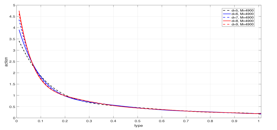
Figure 1: Performance v.s. order of the polynomial $d$, Example 2.

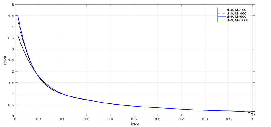
Figure 2: Performance v.s. sample size $M$, Example 2.

Throughout the experiments, the samples are chosen by the discretization scheme discussed in Section 4. For example, in the first set of experiments, we pick up $70$ points evenly spread over $\Theta_{1}$ and $\Theta_{2}$ respectively and use them to form $4900$ grid points over the space of $\Theta_{1}\times\Theta_{2}$. So these samples are generated in a deterministic manner.

Next, we examine the approximation scheme by applying it to an asymmetric rent-seeking contest with both players having identical expected utility functions and action spaces as in Example 2 but with different type sets.

Example 5.2 (Asymmetric rent-seeking contests)

Let $n=2$, $\Theta_{1}=[0.01,1.01]$, $\Theta_{2}=[0.01,2.01]$ and $\mathcal{A}_{1}=\mathcal{A}_{2}=[0,100]$. As in Example 2, we assume that $\theta_{1}$ and $\theta_{2}$ are independent and uniformly distributed over $\Theta_{1}$ and $\Theta_{2}$ respectively. This example is varied from Ewerhart [10] where $\Theta_{2}=[0.51,5.51]$ whereas all other settings are the same.

We have carried out two sets of experiments as in Example 2. The results are depicted in Figures 3 and 4. Figure 3 visualizes changes of the approximate behavioural functions at equilibrium for player 1 and player 2 when the order of the polynomials $d$ increases from $5$ to $8$ with fixed sample size $M=5000$. Figure 4 depicts changes of the approximate behavioural functions at equilibrium when the sample size $M$ changes from $72$ to $392$ with fixed order of the polynomials $d=8$. Note that different from Example 2, the size of interval $\Theta_{2}$ is twice of $\Theta_{1}$, so we pick up $K$ points and $2K$ points evenly from $\Theta_{1}$ and $\Theta_{2}$ with $K=6,10,13,14$ and use them to generate $K\times 2K$ grid points/samples.

The preliminary numerical tests show that our approximation schemes work very well. Note that it is possible to reformulate problem (5.71) into a nonlinear complementarity problem (NCP) through first order optimality conditions and consequently we may replace Algorithm 5.1 with an existing NCP solver such as PATH. Since the reformulation is equivalent, it does not affect the test results but may avoid the iterative process.

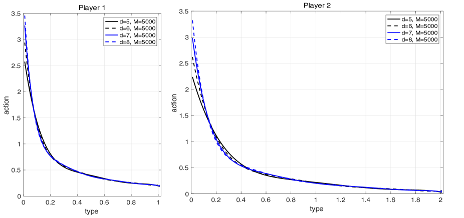
Figure 3: Performance v.s. order of the polynomial $d$, Example 4.

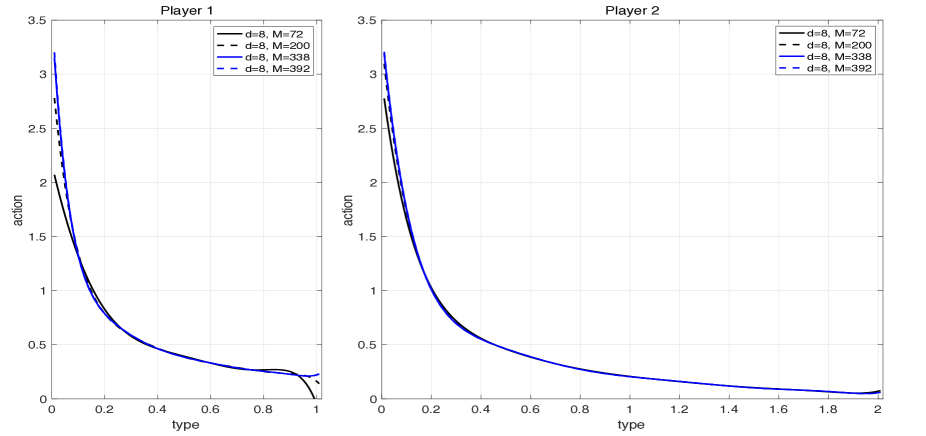
Figure 4: Performance v.s. sample size $M$, Example 4.

References

• [1] M. Aghassi and D. Bertsimas, Robust game theory, Mathematical Programming, Ser. B, 107: 231-273, 2006.
• [2] S. Athey, Single crossing properties and the existence of pure strategy equilibria in games of incomplete information, Econometrica, 69: 861-889, 2001.
• [3] K. B. Athreya and S. N. Lahiri, Measure Theory and Probability Theory, Springer, New York, 2006.
• [4] R. J. Aumann, Integrals of set-valued functions, Journal of Mathematical Analysis and Applications, 12: 1-12, 1965.
• [5] D. Bampou and D. Kuhn. Polynomial approximations for continuous linear programs, SIAM Journal on Optimization, 22: 628-648, 2012.
• [6] B. Bank, J. Guddat, D. Klatte, B. Kummer and K. Tammer, Nonlinear Parametric Optimization, Akademine-Verlag, Berlin, 1982.
• [7] H. Bohnenblust and S. Karlin, On a theorem of Ville. In: H. Kuhn, A. Tucker (eds.), Contributions to the theory of games, Vol. 1, Princeton UP, Princeton, 155-160, 1950.
• [8] J. F. Bonnans and A. Shapiro, Perturbation Analysis of Optimization Problems, Springer, New York, 2000.
• [9] F. H. Clarke, Optimization and nonsmooth analysis, Wiley, New York, 1983.
• [10] C. Ewerhart, Unique equilibrium in rent-seeking contests with a continuum of types, Economics letters, 125: 115-118, 2014.
• [11] C. Ewerhart and F. Quartieri, Unique equilibrium in incomplete information contests with budget constraints, working paper, 2015.
• [12] M. Fey, Rent-seeking contests with incomplete information, Public Choice, 135: 225-236, 2008.
• [13] A. Fischer, M. Herrich and K. Schönefeld, Generalized Nash equilibrium problems-recent advances and challenges, Pesquisa Operacional, 34: 521-558, 2014.
• [14] J. Harsanyi, Games with incomplete information played by ‘Bayesian’ players, parts I-III, Management Science, 14: 159-182, 320-334, 486-502, 1967, 1968.
• [15] S. Kakutani, Generalization of Brouwer’s fixed point theorem. Duke Mathematical Journal 8: 457-459, 1941.
• [16] D. Kuhn, W. Wiesemann and A. Georghiou, Primal and dual linear decision rules in stochastic and robust optimization, Mathematical Programming, 130: 177-209, 2011.
• [17] A. Meirowitz, On the existence of equilibria to Bayesian games with non-finite type and action spaces, Economics Letters, 78: 213-218, 2003.
• [18] G. C. Pflug and A. Pichler, Approximations for probability distributions and stochastic optimization problems, International Series in Operations Research & Management Science, Springer, New York, 163: 343-387, 2011.
• [19] S. M. Robinson, An application of error bounds for convex programming in a linear space, SIAM Journal on Control and Optimization, 13: 271-273, 1975.
• [20] R. T. Rockafellar, Convex Analysis, Princeton University Press, Princeton, 1997.
• [21] A. Shapiro and H. Xu, Stochastic mathematical programs with equilibrium constraints, modeling and sample average approximation, Optimization, 57: 395-418, 2008.
• [22] G. Tullock, Efficient rent seeking. In: J. Buchanan, R. Tollison & G. Tullock (eds.), Toward a theory of the rent-seeking society, College Station: Texas A & M University Press, 97-112, 1980.
• [23] G. Tullock, The welfare costs of tariffs, monopolies, and theft, Western Economic Journal, 5: 224-232, 1967.
• [24] T. Ui, Bayesian Nash equilibrium and variational inequalities, Journal of Mathematical Economics, 63: 139-146, 2016.
• [25] H. Xu and D. Zhang, Stochastic Nash equilibrium problems: sample average approximation and applications, Computational Optimization and Applications, 55: 597-645, 2013.