The Weizsäcker-Williams distribution of linearly polarized gluons (and its fluctuations) at small x

Abstract

The conventional and linearly polarized Weizsäcker-Williams gluon distributions at small $x$ are defined from the two-point function of the gluon field in light-cone gauge. They appear in the cross section for dijet production in deep inelastic scattering at high energy. We determine these functions in the small-$x$ limit from solutions of the JIMWLK evolution equations and show that they exhibit approximate geometric scaling. Also, we discuss the functional distributions of these WW gluon distributions over the JIMWLK ensemble at rapidity $Y\sim 1/\alpha_{s}$. These are determined by a 2d Liouville action for the logarithm of the covariant gauge function $g^{2}\mathrm{tr}\,A^{+}(q)A^{+}(-q)$. For transverse momenta on the order of the saturation scale we observe large variations across configurations (evolution trajectories) of the linearly polarized distribution up to several times its average, and even to negative values.

1 Introduction

Dijet production in deep-inelastic $\gamma^{*}-A$ scattering at high energy can provide insight into the gluon fields of the nucleus in the regime of strong, non-linear fields Aschenauer:2017jsk . At leading order a $q\bar{q}$ dijet is produced. Denote the average transverse momentum of the jets as $\vec{P}=(\vec{k}_{1}-\vec{k}_{2})/2$ and the transverse momentum imbalance as $q=\vec{k}_{1}+\vec{k}_{2}$, where $\vec{k}_{1}$ and $\vec{k}_{2}$ are the transverse momenta of the two jets. In the “correlation limit” of roughly back to back jets Dominguez:2011wm one has $P^{2}\gg q^{2}$. In this limit the leading contribution (in powers of $q^{2}/P^{2}$) to the cross section can be obtained from Transverse Momentum Dependent (TMD) factorization. It predicts a distribution $xh^{(1)}(x,q^{2})$ for linearly polarized gluons in an unpolarized target Mulders:2000sh ; Meissner:2007rx which gives rise to $\sim\cos 2\phi$ azimuthal anisotropies in dijet production Boer:2009nc ; Metz:2011wb ; DQXY , as well as in other processes Boer:2010zf ; Qiu:2011ai ; Lansberg:2017tlc . $\phi$ is the angle between the transverse momentum vectors $\vec{P}$ and $\vec{q}$ (in a frame where neither the $\gamma^{*}$ nor the hadronic target carry transverse momentum). The isotropic contribution to the dijet cross section is proportional to the conventional Weizsäcker-Williams (WW) gluon distribution $xG^{(1)}(x,q^{2})$:

$$E_{1}E_{2}\frac{d\sigma^{\gamma_{T}^{\ast}A\rightarrow q\bar{q}X}}{d^{3}k_{1}d^{3}k_{2}d^{2}b} = \alpha_{em}e_{q}^{2}\alpha_{s}\delta\left(x_{\gamma^{\ast}}-1\right)z(1-z)\left(z^{2}+(1-z)^{2}\right)\frac{\epsilon_{f}^{4}+{P}^{4}}{({P}^{2}+\epsilon_{f}^{2})^{4}}$$ (1)

$$\quad\quad\quad\quad\quad\quad\times\left[xG^{(1)}(x,q)-\frac{2\epsilon_{f}^{2}{P}^{2}}{\epsilon_{f}^{4}+{P}^{4}}\cos\left(2\phi\right)xh^{(1)}(x,q)\right]\leavevmode\nobreak\ ,$$

$$E_{1}E_{2}\frac{d\sigma^{\gamma_{L}^{\ast}A\rightarrow q\bar{q}X}}{d^{3}k_{1}d^{3}k_{2}d^{2}b} = \alpha_{em}e_{q}^{2}\alpha_{s}\delta\left(x_{\gamma^{\ast}}-1\right)z^{2}(1-z)^{2}\frac{8\epsilon_{f}^{2}{P}^{2}}{({P}^{2}+\epsilon_{f}^{2})^{4}}$$ (2)

$$\quad\quad\quad\quad\quad\quad\times\left[xG^{(1)}(x,q)+\cos\left(2\phi\right)xh^{(1)}(x,q)\right]\leavevmode\nobreak\ .$$

$z$ and $1-z$ are the momentum fractions of the quark and anti-quark, respectively, and $\epsilon_{f}^{2}=z(1-z)Q^{2}$ (for massless quarks) with $Q^{2}$ the virtuality of the photon. Clearly, positivity of the cross section imposes the upper bound $|xh^{(1)}(x,q^{2})|\leq xG^{(1)}(x,q^{2})$. Note that even though $P$ is taken to be the hard scale in the process, which can be greater than the saturation scale of the nucleus, that nevertheless the WW gluon distributions are probed at the much smaller momentum imbalance scale $q$. Therefore, the process can indeed provide information on these gluon distributions in the dense regime at $q<Q_{s}$. The WW gluon distributions also determine the divergence of the Chern-Simons current at the initial time in relativistic heavy-ion collisions Lappi:2017skr even though they are not the gluon distributions which enter the cross section for gluon production Kharzeev:2003wz .

In the Color Glass Condensate (CGC) framework at small $x$ the gluon fields are described by Wilson lines. They are path ordered exponentials in the strong color field of the target, and cross sections for different observables can be related to correlators of the Wilson lines. The Wilson line is a path ordered exponential of the covariant gauge field, whose largest component is $A^{+}$:

$$U(\vec{x})=\mathbb{P}\exp\left\{ig\int dx^{-}A^{+}(x^{-},\vec{x})\right\}.$$ (3)

The WW unintegrated gluon distribution Dominguez:2011wm ; Kharzeev:2003wz ; Dominguez:2011br , on the other hand, is defined in terms of the light cone gauge ($A^{+}=0$) field; it can be obtained by a gauge transformation

$${A}^{i}(\vec{x})=\frac{1}{ig}U^{\dagger}(\vec{x})\,\partial_{i}U(\vec{x})\leavevmode\nobreak\ .$$ (4)

The trace (or the traceless part) of the two-point correlator of the light cone gauge field

$$xG^{ij}_{\rm WW}(x,\vec{q})=\frac{1}{A_{\perp}}\frac{1}{2\pi}\left<A^{i}_{a}(\vec{q})A^{j}_{a}(-\vec{q})\right>$$ (5)

defines $xG^{(1)}(x,q^{2})$ and $xh^{(1)}(x,q^{2})$ introduced above:

$$xG^{ij}_{\rm WW}(x,q^{2})=\frac{1}{2}\delta^{ij}xG^{(1)}(x,q^{2})+\frac{1}{2}\left(2\frac{q^{i}q^{j}}{q^{2}}-\delta^{ij}\right)xh^{(1)}(x,q^{2})\leavevmode\nobreak\ .$$ (6)

$A_{\perp}$ in eq. (5) denotes a transverse area over which the gluon distributions have been averaged over.

2 The WW gluon distributions at small $x$

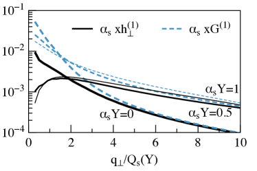
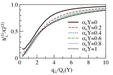
Figure 1: $xG^{(1)}(x,q^{2})$ and $xh^{(1)}(x,q^{2})$ WW gluon distributions versus transverse momentum $q$ at different rapidities $Y$. $Q_{s}(Y)$ is the saturation momentum. The curves correspond to evolution at fixed $\alpha_{s}$.

These WW gluon distributions have been obtained at small $x$ (high rapidity) by a numerical solution of the JIMWLK evolution equations jimwlk in ref. Dumitru:2015gaa , shown in fig. 1. At high transverse momentum one finds that $xh^{(1)}(x,q^{2})\to xG^{(1)}(x,q^{2})$. This is easy to understand from the fact that in the dilute limit the classical light-cone gauge field is given by $A^{i}(q)=ig(q^{i}/q^{2})\rho(q)$ where $g\rho(q)$ denotes the color charge density of the sources. For $A^{i}(q)\sim q^{i}$ eqs. (5,6) give $xh^{(1)}(x,q^{2})=xG^{(1)}(x,q^{2})$. Thus, the saturation of the above-mentioned bound on the distribution of linearly polarized gluons at high transverse momentum is a generic consequence of the dilute semi-classical field limit. On the other hand, at low $q$ one has $xh^{(1)}(x,q^{2})/xG^{(1)}(x,q^{2})\approx 0$ implying that the angular dependence of the cross section (2) is weaker. For more detailed predictions of $\langle\cos 2\phi\rangle$ obtained with the small-$x$ WW gluon distributions see ref. Dumitru:2015gaa .

The numerical solutions also indicate that the WW gluon distributions approach scaling functions $xh^{(1)}(x,q^{2})=xh^{(1)}(q^{2}/Q_{s}^{2}(x))$, $xG^{(1)}(x,q^{2})=xG^{(1)}(q^{2}/Q_{s}^{2}(x))$, at high rapidity. This is known as geometric scaling and has been discussed originally in the context of the dipole forward scattering amplitude (resp. the $\gamma^{*}-p$ total cross section) Stasto:2000er . Geometric scaling of the WW distributions can be motivated from a Gaussian approximation to JIMWLK Iancu:2002aq . In this approximation, and also taking $N_{c}\gg 1$ for simplicity, they can be written in terms of the two-point function $\Gamma(r)$ of $A^{+}$ as Dumitru:2016jku

$$xh^{(1)}(x,q^{2}) = \frac{4N_{c}}{\alpha_{s}(2\pi)^{3}}\int drr^{3}J_{2}(qr)\left(1-[S(r^{2})]^{2}\right)\frac{\Gamma^{\prime\prime}(r^{2})}{\Gamma(r^{2})}$$ (7)

$$xG^{(1)}(x,q^{2}) = \frac{4N_{c}}{\alpha_{s}(2\pi)^{3}}\int drrJ_{0}(qr)\left(1-[S(r^{2})]^{2}\right)\left(\frac{\Gamma^{\prime}(r^{2})}{\Gamma(r^{2})}+r^{2}\frac{\Gamma^{\prime\prime}(r^{2})}{\Gamma(r^{2})}\right)\leavevmode\nobreak\ .$$ (8)

$S(r^{2})=\exp\left(-(1/2)C_{F}\Gamma(r^{2})\right)$ is the S-matrix for a dipole of size $r$. At the JIMWLK fixed point $\Gamma(r^{2})$, $r^{2}\Gamma^{\prime}(r^{2})$, and $r^{4}\Gamma^{\prime\prime}(r^{2})$ are in fact functions of $r^{2}Q_{s}^{2}(x)$ only, rather than functions of both $r$ and $x$. From the above expressions for $xh^{(1)}(x,q^{2})$ and $xG^{(1)}(x,q^{2})$ it follows that these functions then satisfy geometric scaling (also see ref. Marquet:2016cgx ).

3 The JIMWLK weight functional and the constraint effective potential for $g^{2}\mathrm{tr}\,|A^{+}(q)|^{2}$

Expectation values of observables at small $x$ are computed by i) expressing the observable as a functional $O[A^{+}]$ of the covariant gauge field, ii) and averaging over the random semi-classical fields $A^{+}$ with the weight $W_{Y}[A^{+}]$:

$$\langle O\rangle=\frac{1}{Z}\int{\cal D}A^{+}(q)\,W_{Y}[A^{+}(q)]\,O[A^{+}(q)]\leavevmode\nobreak\ \leavevmode\nobreak\ \leavevmode\nobreak\ \leavevmode\nobreak\ ,\leavevmode\nobreak\ \leavevmode\nobreak\ \leavevmode\nobreak\ \leavevmode\nobreak\ Z=\int{\cal D}A^{+}(q)\,W_{Y}[A^{+}(q)]\leavevmode\nobreak\ .$$ (9)

Note that $A^{+}(q)$ is the soft semi-classical field which solves the Poisson equation, $A^{+}(q)=g\rho(q)/q^{2}$, with $g\rho(q)$ the random, effective color charge density that is the source of the soft gluon field. Hence, the above average over $A^{+}$ can also be written as an average over $\rho$.

The weight $W_{Y}[A^{+}(q)]$ for a given configuration $A^{+}(q)$ is determined by the solution of the JIMWLK functional RG equation jimwlk . The exact solution can only be obtained numerically. However, a non-local (in coordinate space) Gaussian mean-field approximation for $W_{Y}[\rho]$ has been proposed, see first reference in Iancu:2002aq , which reproduces the proper gluon distribution $g^{2}\mathrm{tr}\,A^{+}(q)\,A^{+}(-q)$ both at small ($q^{2}\ll Q_{s}^{2}$) as well as at high ($q^{2}\gg Q_{s}^{2}$) transverse momentum:

$$W_{G}[A^{+}]=e^{-S_{G}[A^{+}]}\leavevmode\nobreak\ \leavevmode\nobreak\ \leavevmode\nobreak\ ,\leavevmode\nobreak\ \leavevmode\nobreak\ \leavevmode\nobreak\ S_{G}[A^{+}]=\int\frac{\mathrm{d}^{2}q}{(2\pi)^{2}}\,q^{4}\frac{\mathrm{tr}\,A^{+}(q)\,A^{+}(-q)}{g^{2}\mu^{2}(q^{2})}\leavevmode\nobreak\ .$$ (10)

For simplicity we restrict here to high transverse momentum where

$$\mu^{2}(q^{2})\simeq\mu_{0}^{2}\left(\frac{q^{2}}{Q_{s}^{2}}\right)^{1-\gamma}\leavevmode\nobreak\ ,$$ (11)

with $\gamma\simeq 0.64$ an anomalous dimension Mueller:2002zm . $Q_{s}^{2}$ and $\mu_{0}^{2}\sim A^{1/3}$ are evaluated at the rapidity of interest but we will not spell out this dependence on $Y$ explicitly.

The expectation value of $O[A^{+}]$ written in eq. (9) is an average over all configurations of $A^{+}(q)$. However, one may be interested in evaluating $\langle O\rangle$ over a subclass of configurations, for example those with a high (or low) number of gluons, or with an unusual transverse momentum distribution of gluons. To that end we introduce the constraint effective potential for $X(q)=g^{2}\mathrm{tr}\,|A^{+}(q)|^{2}$ by integrating over configurations at fixed $X(q)$ Dumitru:2017cwt :

$$Z = \int{\cal D}X(q)\,e^{-V_{\mathrm{eff}}[X(q)]}\leavevmode\nobreak\ ,$$ (12)

$$e^{-V_{\mathrm{eff}}[X(q)]} = \int{\cal D}A^{+}(q)\,W_{Y}[A^{+}(q)]\,\delta(X(q)-g^{2}\mathrm{tr}\,|A^{+}(q)|^{2})\leavevmode\nobreak\ .$$ (13)

For a Gaussian theory the integral over configurations at fixed $X(q)$ is easy to compute, and the resulting effective potential is Dumitru:2017cwt

$$V_{\mathrm{eff}}[X(q)]=\int\frac{\mathrm{d}^{2}q}{(2\pi)^{2}}\left[\frac{q^{4}}{g^{4}\mu^{2}(q)}X(q)-\frac{1}{2}A_{\perp}N_{c}^{2}\log X(q)\right]\leavevmode\nobreak\ ,$$ (14)

$A_{\perp}$ is the transverse area over which

$$\mathrm{tr}\,|A^{+}(q)|^{2}=\int_{A_{\perp}}{\mathrm{d}^{2}b}\int{\mathrm{d}^{2}r}\,e^{-i\vec{q}\cdot\vec{r}}A^{+}(\vec{b}-\vec{r}/2)A^{+}(\vec{b}+\vec{r}/2)$$ (15)

has been integrated. The stationary point of $V_{\mathrm{eff}}[X]$ determines the extremal gluon distribution

$$X_{s}(q)=\frac{1}{2}N_{c}^{2}A_{\perp}\frac{g^{4}\mu^{2}(q)}{q^{4}}\leavevmode\nobreak\ .$$ (16)

$X_{s}(q)$ is the most likely gluon distribution function rather than the average. However, in the large-$N_{c}$ limit it is equal to the expectation value of $\langle g^{2}\mathrm{tr}\,|A^{+}(q)|^{2}\rangle$. Away from the extremal solution, the potential $V_{\mathrm{eff}}[X]$ provides insight into the distribution of functions $X(q)$ about the extremum. This distribution is determined by a “linear minus logarithmic” rather than by a polynomial potential.

It will be convenient for what follows to describe deviations from $X_{s}(q)$ by multiplying with $\eta(q)$ rather than by adding $\delta X(q)$. Hence, we introduce the function $\eta(q)$ through $X(q)=X_{s}(q)\,\eta(q)$. A fluctuation from the extremal field $X_{s}(q)$ has action

$$V_{\mathrm{eff}}[\eta(q)]=\frac{1}{2}N_{c}^{2}A_{\perp}\int\frac{\mathrm{d}^{2}q}{(2\pi)^{2}}\left[\eta(q)-1-\log\eta(q)\right]\leavevmode\nobreak\ .$$ (17)

Note that $X(q)=g^{2}\mathrm{tr}\,|A^{+}(q)|^{2}$ is a positive definite function and so is $\eta(q)$. We can therefore perform another field redefinition to introduce $\phi(q)$ through $e^{\phi(q)}=\eta(q)$ so that

$$V_{\mathrm{eff}}[\phi(q)]=\frac{1}{2}N_{c}^{2}A_{\perp}\int\frac{\mathrm{d}^{2}q}{(2\pi)^{2}}\left[e^{\phi(q)}-\phi(q)-1\right]\leavevmode\nobreak\ .$$ (18)

Thus, we found that it is a Liouville action in two dimensions which describes the distribution of $\log\mathrm{tr}\,|gA^{+}(q)|^{2}$ (relative to the average gluon distribution) in a Gaussian approximation to JIMWLK.

The action for the most likely distribution function $X_{s}(q)$ is of order $N_{c}^{2}A^{1/3}$ (times zero, in dimensional regularization). So is the action for $X(q)=X_{s}(q)\eta(q)$ if $\eta(q)={\cal O}(1)$. Our discussion is restricted to the distribution of functions $X(q)$ which exhibit longitudinal coherence and are of order $N_{c}^{2}A^{1/3}$. The small-$x$ power counting assumes $g^{4}A^{1/3}={\cal O}(1)$ Kovchegov:1999ua , and so $X(q)\sim(A^{1/3})^{0}$ would correspond to a higher order correction in the coupling.

Knowing $V_{\mathrm{eff}}$ we can now evaluate the suppression probability for a modification of the gluon distribution such as

$$\eta(q)=1+\eta_{0}\left(\frac{g^{4}\mu_{0}^{2}}{q^{2}}\right)^{a}\,\Theta\left(q^{2}-\Lambda^{2}\right)\Theta\left(Q^{2}-q^{2}\right)\leavevmode\nobreak\ .$$ (19)

$\eta_{0}$ determines the amplitude of the distortion, $Q^{2}$ and $\Lambda^{2}>Q_{s}^{2}$ determine its support, and the parameter $a$ specifies the spectral shape. The action for such $\eta(q)$ when $Q^{2}\gg\Lambda^{2}$ is

$$V_{\mathrm{eff}}[\eta(q)]\simeq\frac{1}{8\pi}N_{c}^{2}A_{\perp}\,g^{4}\mu_{0}^{2}\,\eta_{0}\times\begin{cases}\frac{1}{1-a}\left(\frac{Q^{2}}{g^{4}\mu_{0}^{2}}\right)^{1-a}&(a<1)\leavevmode\nobreak\ ,\\ \log\frac{Q^{2}}{\Lambda^{2}}&(a=1)\leavevmode\nobreak\ ,\\ \frac{1}{a-1}\left(\frac{g^{4}\mu_{0}^{2}}{\Lambda^{2}}\right)^{a-1}&(a>1)\leavevmode\nobreak\ .\end{cases}$$ (20)

Hence, we find that a harder than average gluon distribution ($a<0$) over $\Lambda<q<Q$ comes at a high price since $V_{\mathrm{eff}}[\eta(q)]\sim(Q^{2}/g^{4}\mu_{0}^{2})^{1-a}$. On the other hand, gluon distributions which drop substantially faster than the most likely one (i.e. $X_{s}(q)$) correspond to $a\geq 1$, and such fluctuations can extend to high transverse momentum. For a more detailed discussion of the shape of the gluon distribution in the presence of a high (or low) gluon multiplicity “trigger” we refer to ref. Dumitru:2017cwt .

4 The functional distribution of WW gluon distributions over the JIMWLK ensemble

In sec. 2 we discussed the WW gluon distributions averaged over the entire JIMWLK ensemble $W_{Y}[A+]$. In this section we discuss the distributions of these functions over the JIMWLK ensemble.

To obtain some basic analytic insight we write the expansion of $g^{2}\mathrm{tr}\,A^{i}(q)A^{j}(-q)$ to fourth order in $A^{+}(q)$ obtained via eq. (4):

$$\delta^{ij}\mathrm{tr}\,A^{i}(q)A^{j}(-q) = \frac{1}{2}q^{2}A^{+a}(q)A^{+a}(-q)$$ (21)

$$+\frac{g^{2}}{8}f^{abe}f^{cde}\left(\frac{q^{n}q^{m}}{q^{2}}-\delta^{nm}\right)\int\frac{\mathrm{d}^{2}k}{(2\pi)^{2}}k^{n}A^{+a}(q-k)A^{+b}(k)\int\frac{\mathrm{d}^{2}p}{(2\pi)^{2}}p^{m}A^{+c}(-q-p)A^{+d}(p)\leavevmode\nobreak\ ,$$

$$\left(2\frac{q^{i}q^{j}}{q^{2}}-\delta^{ij}\right)\mathrm{tr}\,A^{i}(q)A^{j}(-q) = \frac{1}{2}q^{2}A^{+a}(q)A^{+a}(-q)$$ (22)

$$-\frac{g^{2}}{8}f^{abe}f^{cde}\left(\frac{q^{n}q^{m}}{q^{2}}-\delta^{nm}\right)\int\frac{\mathrm{d}^{2}k}{(2\pi)^{2}}k^{n}A^{+a}(q-k)A^{+b}(k)\int\frac{\mathrm{d}^{2}p}{(2\pi)^{2}}p^{m}A^{+c}(-q-p)A^{+d}(p)\leavevmode\nobreak\ .$$

In the weak-field limit the first term in these expansions dominates and the two WW gluon distributions are equal, configuration by configuration. The correction at fourth power in $A^{+}$ generates a “splitting”. We can perform an average over a Gaussian ensemble by summing the two non-vanishing Wick contractions using

$$\left<A^{+a}(q)\,A^{+b}(k)\right>=\delta^{ab}\,(2\pi)^{2}\delta(q+k)\frac{g^{2}\mu^{2}(q^{2})}{q^{4}}\leavevmode\nobreak\ .$$ (23)

At order $N_{c}^{2}$ this leads to

$$\delta^{ij}\,g^{2}\left<\mathrm{tr}\,A^{i}(q)A^{j}(-q)\right>=\frac{1}{2}N_{c}^{2}A_{\perp}\frac{g^{4}\mu^{2}(q)}{q^{2}}+N_{c}^{3}A_{\perp}\frac{g^{8}}{4}\int\frac{\mathrm{d}^{2}k}{(2\pi)^{2}}k^{2}\left[1-(\hat{k}\cdot\hat{q})^{2}\right]\frac{\mu^{2}(q-k)}{(q-k)^{4}}\frac{\mu^{2}(k)}{k^{4}}\leavevmode\nobreak\ .$$ (24)

The result for the average of eq. (22) is the same except that the sign of the second term is negative. Thus, one may wonder if the linearly polarized distribution could take negative values. It is clear that at high $q^{2}$ the correction is $\sim 1/q^{2}$ power suppressed as compared to the leading contribution. This suppression ensures that $xh^{(1)}(x,q^{2})$, averaged over all configurations, is a positive definite function (as seen in fig. 1).

Instead of averaging over all JIMWLK configurations we can use the approach from the previous section to integrate over all configurations at fixed $X(q)=g^{2}\mathrm{tr}\,|A^{+}(q)|^{2}$. To do so, instead of using eq. (23) we make the final integration over $X(q)$ explicit:

$$\left<A^{+a}(q)\,A^{+b}(k)\right>=\delta^{ab}\,(2\pi)^{2}\delta(q+k)\frac{g^{2}\mu^{2}(q^{2})}{q^{4}}\int{\cal D}X(\ell)\,e^{-V_{\mathrm{eff}}[X(\ell)]}\,\frac{X(q)}{X_{s}(q)}\leavevmode\nobreak\ .$$ (25)

We can then rewrite eq. (24) as follows:

$$\delta^{ij}\,g^{2}\left<\mathrm{tr}\,A^{i}(q)A^{j}(-q)\right> = q^{2}\int{\cal D}X(\ell)\,e^{-V_{\mathrm{eff}}[X(\ell)]}\,X(q)$$ (26)

$$+\frac{1}{N_{c}A_{\perp}}\int\frac{\mathrm{d}^{2}k}{(2\pi)^{2}}k^{2}\left[1-(\hat{k}\cdot\hat{q})^{2}\right]\int{\cal D}X(\ell)\,e^{-V_{\mathrm{eff}}[X(\ell)]}\,X(q-k)X(k)\leavevmode\nobreak\ .$$

As before, replacing the projector $\delta^{ij}$ by $2{q^{i}q^{j}}/{q^{2}}-\delta^{ij}$ reverses the sign of the last term. It is evident that for some functions $X(q)$ which contribute to the integral the correction in this last expression may be greater than the “leading” contribution. These configurations overcome the power suppression discussed above which arises at the saddle point of the integral; also, they give linearly polarized gluon distributions which are negative in some range of transverse momentum.

We now show some numerical results obtained by Monte-Carlo sampling of the JIMWLK functional $W_{Y}[A^{+}]$ Dumitru:2017cwt for $N_{c}=3$ colors and fixed $\alpha_{s}$. We evaluate the WW gluon distributions on each configuration. They have to be integrated over a finite patch in impact parameter space greater than the inverse transverse momentum. We take

$$P^{ij}\int{\mathrm{d}^{2}x}{\mathrm{d}^{2}y}\,e^{-iq\cdot(x-y)}e^{-(x^{2}+y^{2})/2R^{2}}\,g^{2}\mathrm{tr}\,A^{i}(x)A^{j}(y)\leavevmode\nobreak\ ,$$ (27)

with $R=2/Q_{s}(Y)$ and $q>Q_{s}(Y)$ the transverse momentum scale. $P^{ij}$ denotes one of the two projectors mentioned above. This expression factorizes into a product of two Fast Fourier Transforms which can be evaluated numerically very efficiently.

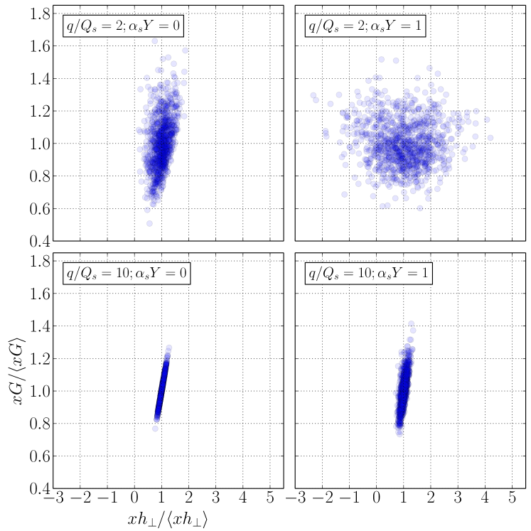
Figure 2: $xG^{(1)}(x,q^{2})$ and $xh^{(1)}(x,q^{2})$ WW gluon distributions for 1000 individual field configurations, evaluated at $q=2Q_{s}(Y)$ or $q=10Q_{s}(Y)$, respectively. Notice the different scales on the horizontal and vertical axes. Left: MV model initial condition; Right: JIMWLK ensemble at $\alpha_{s}Y=1$.

In fig. 2 we show the $xG^{(1)}(x,q^{2})$ and $xh^{(1)}(x,q^{2})$ WW gluon distributions for individual configurations, relative to their average. For high transverse momentum far above $Q_{s}(Y)$ we observe, as expected, that the two functions are essentially equal, even for individual configurations. For $q=2Q_{s}(Y)$ on the other hand the relative fluctuations of the linearly polarized distribution are much greater than those of the conventional WW distribution. For some configurations $xh^{(1)}(x,q^{2})$ can take values up to several times its average while other evolution trajectories lead to negative values. This is an effect of evolution to small $x$ since $xh^{(1)}(x,q^{2})<0$ at $q=2Q_{s}(Y)$ does not occur at $Y=0$ once in $10^{4}$ configurations.

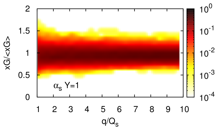
Figure 3: Distribution of functions $xG^{(1)}(x,q^{2})/\langle xG^{(1)}(x,q^{2})\rangle$ in the JIMWLK ensemble at $\alpha_{s}Y=1$. The color coding indicates the probability for a particular function $xG^{(1)}(x,q^{2})/\langle xG^{(1)}(x,q^{2})\rangle$.

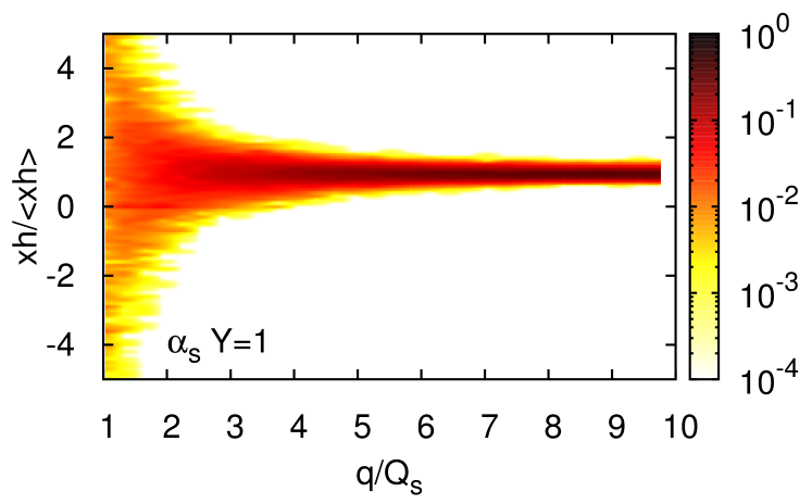
Figure 4: Distribution of functions $xh^{(1)}(x,q^{2})/\langle xh^{(1)}(x,q^{2})\rangle$ in the JIMWLK ensemble at $\alpha_{s}Y=1$.

The functional distributions of $xG^{(1)}(x,q^{2})$ and $xh^{(1)}(x,q^{2})$ in the JIMWLK ensemble are shown in figs. 3 and 4, respectively. At high transverse momentum the distributions are strongly peaked about the most likely WW functions. On the other hand, when $q$ is not very far above $Q_{s}(Y)$ the ensemble of linearly polarized WW gluon distribution functions is broad. At $\alpha_{s}Y\sim 1$ it includes non-positive definite functions as well as functions which take values several times their average.

References

(1)
E. C. Aschenauer et al.,
arXiv:1708.01527 [nucl-ex].
(2)
F. Dominguez, C. Marquet, B. W. Xiao and F. Yuan,
Phys. Rev. D 83, 105005 (2011)
(3)
P. J. Mulders and J. Rodrigues,
Phys. Rev. D 63, 094021 (2001)
(4)
S. Meissner, A. Metz and K. Goeke,
Phys. Rev. D 76, 034002 (2007)
(5)
D. Boer, P. J. Mulders and C. Pisano,
Phys. Rev. D 80, 094017 (2009)
(6)
A. Metz and J. Zhou,
Phys. Rev. D 84, 051503 (2011)
(7)
F. Dominguez, J. W. Qiu, B. W. Xiao and F. Yuan,
Phys. Rev. D 85, 045003 (2012)
(8)
D. Boer, S. J. Brodsky, P. J. Mulders and C. Pisano,
Phys. Rev. Lett. 106, 132001 (2011)
(9)
J. W. Qiu, M. Schlegel and W. Vogelsang,
Phys. Rev. Lett. 107, 062001 (2011)
(10)
J. P. Lansberg, C. Pisano and M. Schlegel,
Nucl. Phys. B 920, 192 (2017);
J. P. Lansberg, C. Pisano, F. Scarpa and M. Schlegel,
arXiv:1710.01684 [hep-ph].
(11)
T. Lappi and S. Schlichting,
arXiv:1708.08625 [hep-ph].
(12)
D. Kharzeev, Y. V. Kovchegov and K. Tuchin,
Phys. Rev. D 68, 094013 (2003)
(13)
F. Dominguez, J. W. Qiu, B. W. Xiao and F. Yuan,
Phys. Rev. D 85, 045003 (2012)
(14)
J. Jalilian-Marian, A. Kovner, A. Leonidov and H. Weigert,
Nucl. Phys. B 504, 415 (1997);
Phys. Rev. D 59, 014014 (1998);
E. Iancu, A. Leonidov and L. D. McLerran,
Phys. Lett. B 510, 133 (2001);
Nucl. Phys. A 692, 583 (2001);
H. Weigert,
Nucl. Phys. A 703, 823 (2002)
(15)
A. Dumitru, T. Lappi and V. Skokov,
Phys. Rev. Lett. 115, no. 25, 252301 (2015)
(16)
A. M. Stasto, K. J. Golec-Biernat and J. Kwiecinski,
Phys. Rev. Lett. 86, 596 (2001)
(17)
E. Iancu, K. Itakura and L. McLerran,
Nucl. Phys. A 724, 181 (2003);
J. Jalilian-Marian and Y. V. Kovchegov,
Phys. Rev. D 70, 114017 (2004);
H. Fujii, F. Gelis and R. Venugopalan,
Nucl. Phys. A 780, 146 (2006);
C. Marquet and H. Weigert,
Nucl. Phys. A 843, 68 (2010);
E. Iancu and D. N. Triantafyllopoulos,
JHEP 1204, 025 (2012)
(18)
A. Dumitru and V. Skokov,
Phys. Rev. D 94, no. 1, 014030 (2016)
(19)
C. Marquet, E. Petreska and C. Roiesnel,
JHEP 1610, 065 (2016)
(20)
A. H. Mueller and D. N. Triantafyllopoulos,
Nucl. Phys. B 640, 331 (2002)
(21)
A. Dumitru and V. Skokov,
Phys. Rev. D 96, 056029 (2017)
(22)
Y. V. Kovchegov,
Phys. Rev. D 61, 074018 (2000)