Solitons and breathers for nonisospectral mKdV equation with Darboux transformation

Abstract

Under investigation in this paper is the nonisospectral and variable coefficients modified Kortweg-de Vries (vc-mKdV) equation, which manifests in diverse areas of physics such as fluid dynamics, ion acoustic solitons and plasma mechanics. With the degrees of restriction reduced, a simplified constraint is introduced, under which the vc-mKdV equation is an integrable system and the spectral flow is time-varying. The Darboux transformation for such equation is constructed, which gives rise to the generation of variable kinds of solutions including the double-breather coherent structure, periodical soliton-breather and localized solitons and breathers. In addition, the effect of variable coefficients and initial phases is discussed in terms of the soliton amplitude, polarity, velocity and width, which might provide feasible soliton management with certain conditions taken into account.

PACS numbers: 05.45.Yv, 02.30.Ik, 47.35.Fg

Keywords: Nonisospectral modified Korteweg-de Vries equation; Darboux transformation; Breather; Soliton management

I. Introduction

The modified Kortweg-de Vries (mKdV) type equations arise in diverse areas of physics, including fluid dynamics, ion acoustic solitons and plasma mechanics [1, 3, 5, 4, 2]. For instance, the dynamics of the interfacial waves in a two-layer fluid of slowly varying depth is studied by the formulated standard mKdV equation [3], the ion-acoustic solitary waves in certain unmagnetized plasma is described by the cylindrical and spherical mKdV equation [4] and the propagation of circularly polarized few-cycle pulses with wave polarization is investigated by a non-integrable complex mKdV equation [5]. With the inhomogeneous environmental density and boundary conditions taken into account [6], the constant coefficients mKdV equation can be extended as followings:

$$\hskip 28.45274ptu_{t}\,+a(t)\,u^{2}\,u_{x}+b(t)\,u_{xxx}+[c_{0}(t)+c_{1}(t)x]\,u_{x}+d(t)\,u=0\,,$$ (1)

where a(t), b(t), $c_{0}(t),c_{1}(t)$ and d(t) are functions of variable t.

With different selections of coefficients, Eq. (1) has been investigated for physical interest [7, 8, 9, 10]. Thereinto, periodic wave solutions are constructed in bilinear forms based on a multidimensional Riemann theta function [7], group classification is carried out and all the classes under consideration are normalized [8], the pulse waves in thin walled prestressed elastic blood vessels is described [9] and a modified perturbation technique is applied to the problem of the structural instability of algebraic solitons [10].

For constructing soliton solutions from the soliton equations like Eq. (1), there exist many methods such as Hirota bilinear method [11, 12, 13], associated scattering problem [14] and Darboux transformation (DT) [15, 16, 17, 18, 19], in which the DT has proven itself a purely algebraic iterative tool [15, 16]. The main difficulty in finding a proper spectral problem of constructing DT has been investigated and many spectral problems have been searched for, including different forms of DT of Eq. (1) under certain conditions [17, 16, 18, 19].

Except for soliton solutions, Eq. (1) also has solutions in the form of oscillating packets (breathers) [10], which along with the solitons, determine the asymptotics of the wave field [20]. It is believed that some temporal and spatial variability that has been observed in oceanic internal soliton fields may be due to the breather interaction [21] and several investigations have been carried out [21, 22, 23, 20]. The circumstances supporting the formation of breathers are determined with various piecewise-constant initial conditions [22], some detailed examinations of the breather-soliton interaction process are analyzed by the Hirota bilinear method [21] and the breather in numerical simulations using the full nonlinear Euler equations for stratified fluid is presented under several forms of the initial disturbance [23].

Meanwhile, Eq. (1) becomes integrable when the variable coefficients satisfy certain constraint conditions, in which $a(t)=6\,b(t)$ and $d(t)=c_{1}(t)$, leading to analytical discussion related to different branches of physics [24, 25, 11, 26, 27, 28, 29]. Different from above investigation, hereby we introduce a constraint reducing the degrees of restriction

$$\hskip 28.45274pta(t)=6\,b(t)\,e^{\int{\!2\,[d(t)-c_{1}(t)]dt}}\,,$$ (2)

under which Eq. (1) is an integrable system and there can be an integrable constant which is normalized to be 1 in this case.

However, to our best knowledge, the Lax pair and DT for Eq. (1) under constraint (2) have not been obtained. Therefore, in this paper, we will construct the DT with spectral problem for Eq. (1) and generate multi-soliton and breather solutions from the seed ones.

The outline of the present paper is as follows. In Section II and III, the Lax pair and DT for Eq. (1) under constraint (2) are constructed respectively. In Section IV, one-soliton solution is generated by a DT and the characteristic line with soliton amplitude is given. In Section V, two-soliton and three-soliton solutions are investigated analytically by appropriate selection of variable coefficients. In Section VI, different kinds of breathers as well as the interaction between breather and soliton are thrived, including the double-breather coherent structure, periodical soliton-breather and localized breathers. In Section VII, the conclusions are given.

II. Lax pair

Based on AKNS procedure [18], the Lax pair of Eq. (1) under the general constraint (2) is constructed with the undetermined coefficients corresponding to time and space

$$\Phi_{x}(x,t)=U\Phi(x,t)=\left(\begin{array}[]{ccc}\lambda(t)&l(t)\,u\\ -l(t)\,u&-\lambda(t)\\ \end{array}\right)\Phi(x,t),$$ (3)

$$\Phi_{t}(x,t)=V\Phi(x,t)=\left(\begin{array}[]{ccc}A(x,t)&B(x,t)\\ S(x,t)&-A(x,t)\\ \end{array}\right)\Phi(x,t),$$ (4)

where $\Phi(x,t)=(\Phi_{1}(x,t),\Phi_{2}(x,t))^{\textit{T}}\,$ with T representing the transpose of the vector. The $\Phi(x,t)$ should comply with the compatibility condition, which leads to a zero curvature equations [15]

$$\hskip 28.45274ptU_{x}-V_{t}+[U,V]=0.$$ (5)

Substituting Eqs. (3) and (4) into the zero curvature equations and comparing the coefficients of the power of $\lambda(t)$, we have

$$\hskip 28.45274ptl(t)=e^{\int{\![d(t)-c_{1}(t)]dt}},$$ (6)

$$\hskip 28.45274ptA(x,t)=-\big{(}2\,e^{2\,\int{\![d(t)-c_{1}(t)]dt}}\,b(t)\,u^{2}+c_{0}(t)+x\,c_{1}(t)\big{)}\,\lambda(t)-4\,b(t)\,\lambda^{3}(t),$$ (7)

$$\hskip 28.45274ptB(x,t)=-e^{\int{\![d(t)-c_{1}(t)]dt}}\,\big{(}2\,e^{2\,\int{\![d(t)-c_{1}(t)]dt}}\,b(t)\,u^{3}+c_{0}(t)\,u$$ (8)

$$+x\,c_{1}(t)\,u+4\,b(t)\,\lambda^{2}(t)\,u+2\,b(t)\,\lambda(t)\,u_{x}+b(t)\,u_{xx}\big{)}\,,$$

$$\hskip 28.45274ptC(x,t)=e^{\int{\![d(t)-c_{1}(t)]dt}}\,\big{(}2\,e^{2\,\int{\![d(t)-c_{1}(t)]dt}}\,b(t)\,u^{3}+c_{0}(t)\,u$$ (9)

$$+x\,c_{1}(t)\,u+4\,b(t)\,\lambda^{2}(t)\,u-2\,b(t)\,\lambda(t)\,u_{x}+b(t)\,u_{xx}\big{)}\,.$$

Meanwhile, spectral parameter $\lambda(t)$ should satisfy the following relation

$$\hskip 28.45274pt\lambda^{\prime}(t)+c_{1}(t)\,\lambda(t)=0.$$ (10)

III. Construction of DT

Now we introduce a gauge transformation for the spectral problem

$$\hskip 28.45274pt\overline{\Phi}=M\,\Phi\,,$$ (11)

where $M$ is defined by

$$\hskip 28.45274ptM_{x}+M\,U=\overline{U}\,M$$ (12)

$$\hskip 28.45274ptM_{t}+M\,V=\overline{V}\,M$$ (13)

The gauge transformation is called DT [17], if the spectral problem (3) and (4) can be transformed into

$$\overline{\Phi}_{x}=\overline{U}\,\overline{\Phi},$$ (14)

$$\overline{\Phi}_{t}=\overline{V}\,\overline{\Phi},$$ (15)

where $\overline{V}$ and $\overline{U}$ has the same form as U and V and the old potential $u$ is mapped into a new potential $u_{1}$.

Suppose

$$M=\,m(t)\,\lambda(t)\left(\begin{array}[]{ccc}1&0\\ 0&1\\ \end{array}\right)+n(t)\,\lambda_{1}(t)\left(\begin{array}[]{ccc}a_{0}(x,t)&b_{0}(x,t)\\ c_{0}(x,t)&d_{0}(x,t)\\ \end{array}\right),$$ (16)

where $\lambda_{1}(t)=e^{\int{\![-c_{1}(t)]dt}}\,\overline{\lambda_{1}}$.

Substituting Expression (16) into Eqs. (14) and (15), by a direct calculation, we have

$$\hskip 28.45274ptm(t)=n(t)=e^{\int{\![c_{1}(t)]dt}}\,,$$ (17)

$$\hskip 28.45274pta_{0}(x,t)=-d_{0}(x,t)=\frac{f_{2}^{2}-f_{1}^{2}}{f_{1}^{2}+f_{2}^{2}}\,,$$ (18)

$$\hskip 28.45274ptb_{0}(x,t)=c_{0}(x,t)=-\frac{2\,f_{1}\,f_{2}}{f_{1}^{2}+f_{2}^{2}}\,,$$ (19)

where $\Big{(}f_{1}\big{(}x,t,\lambda_{1}(t)\big{)},f_{2}\big{(}x,t,\lambda_{1}(t)\big{)}\Big{)}^{\textit{T}}=\Big{(}\Phi_{1}(x,t),\Phi_{2}(x,t)\Big{)}^{\textit{T}}\,$.

The transformation between old potentials $u$ and new ones $u_{1}$ is given as below

$$\hskip 28.45274ptu_{1}(x,t)=u(x,t)+4\,e^{\int{\![c_{1}(t)-d(t)]dt}}\,\lambda_{1}(t)\,\frac{f_{1}\,f_{2}}{f_{1}^{2}+f_{2}^{2}}\,.$$ (20)

So far, we have obtained the DT (16)-(20), which transforms the matrix spectral problem into another spectral problem of the same type and can generate new solutions from seed ones by purely algebraic iteration.

It is worth noting with certain modification, the DT can be extended as following

$$T=\,e^{\int{\![c_{1}(t)]dt}}\,\lambda(t)\left(\begin{array}[]{ccc}1&0\\ 0&1\\ \end{array}\right)-e^{\int{\![c_{1}(t)]dt}}\,\frac{\lambda_{1}(t)}{1+\sigma^{2}}\left(\begin{array}[]{ccc}1-\sigma^{2}&2\,\sigma\\ 2\,\sigma&-1+\sigma^{2}\\ \end{array}\right)\,,$$ (21)

$$\hskip 28.45274ptu_{1}(x,t)=u(x,t)+4\,e^{\int{\![c_{1}(t)-d(t)]dt}}\,\lambda_{1}(t)\frac{\sigma}{1+\sigma^{2}}\,,$$ (22)

$$\hskip 28.45274pt\sigma=\frac{f_{22}+\mu_{1}\,f_{21}}{f_{12}+\mu_{1}\,f_{11}}\,,$$ (23)

where $\Big{(}f_{11}\big{(}x,t,\lambda_{1}(t)\big{)},f_{21}\big{(}x,t,\lambda_{1}(t)\big{)}\Big{)}^{\textit{T}}$ and $\Big{(}f_{12}\big{(}x,t,\lambda_{1}(t)\big{)},f_{22}\big{(}x,t,\lambda_{1}(t)\big{)}\Big{)}^{\textit{T}}$ are linearly independent solutions of spectral problems.

IV. One soliton solution

Employing $u=0$ as the original solution for Eq. (1), we can obtain the solutions of spectral problems (3) and (4) as below

$$\hskip 28.45274pt\Phi_{1}(x,t)=e^{\Lambda(x,t)}\,,$$ (24)

$$\hskip 28.45274pt\Phi_{2}(x,t)=e^{-\Lambda(x,t)}\,,$$ (25)

$$\hskip 28.45274pt\Lambda(x,t)=\lambda(t)\,x-\int{\![c_{0}(t)\,\lambda(t)+4\,b(t)\,\lambda^{3}(t)]dt}-\xi\,,$$ (26)

where $\xi$ is an integration constant representing soliton initial phase, in every iteration which can change to a certain value.

For a given spectral parameters $\lambda_{1}(t)$ and initial phase $\xi_{1}$ , the explicit solutions $\Big{(}f_{1}\big{(}x,t,\lambda_{1}(t)\big{)},\\ f_{2}\big{(}x,t,\lambda_{1}(t)\big{)}\Big{)}^{\textit{T}}$ can be obtained in terms of Expressions (24)-(26), which leads to a new one soliton solution with the aid of DT (20)

$$\hskip 28.45274ptu_{1}(x,t)=2\,e^{\int{[-d(t)+c_{1}(t)]dt}}\,\lambda_{1}(t)\operatorname{Sech}{\big{[}2\,\Omega(x,t)\big{]}}\,,$$ (27)

where

$$\hskip 14.22636pt\Omega(x,t)=k(t)\,x-w(t)+\xi_{1}\,,$$ (28)

$$\hskip 14.22636ptk(t)=\lambda_{1}(t)\,,$$ (29)

$$\hskip 14.22636ptw(t)=\lambda_{1}(t)\,e^{\int{c_{1}(t)dt}}\,\int{\big{[}\,e^{-\int{c_{1}(t)dt}}(4\,\lambda_{1}^{2}(t)\,b(t)+c_{0}(t))\,\big{]}dt}\,,$$ (30)

Meanwhile, the soliton amplitude and characteristic line can be respectively derived as

$$\hskip 14.22636ptA=2\,e^{\int{[-d(t)+c_{1}(t)]dt}}\,\lambda_{1}(t)=2\,\overline{\lambda_{1}}\,e^{\int{-d(t)dt}}\,,$$ (31)

$$\hskip 14.22636ptk(t)\,x-w(t)+\xi_{1}=0\\ ,$$ (32)

which indicates one soliton amplitude is only affected by $d(t)$ when $\overline{\lambda_{1}}$ is given. It is worth noting that the polarity of soliton also refers to the sign of A. Meanwhile, the soliton velocity can be obtained by the derivation of Expression (32).

V. Multi-soliton solutions

For general application in various fields related to soliton dynamics, we need to consider two soliton interaction, which can be generated by a second DT based on the one-soliton solution. For soliton characters describing their physical features, soliton polarity (or phase) should be taken into account. It is worth mentioning that two soliton polarities are allowed in the mKdV framework due to the isotropic nonliearity [20] and the bipolar soliton interaction plays a role in obtaining soliton management. Therefore, with a positive coefficient $a(t)$ of the cubic nonlinear term in Eq. (1), the effect of initial phase on the soliton polarities will be discussed in the following section.

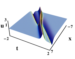
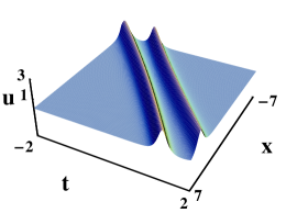
($a$)                                                                                    ($b$)

Fig.  1: Solitonic propagation and interaction with coefficients $\overline{\lambda_{1}}=1$, $\overline{\lambda_{2}}=1.1$, $b(t)=1$, $c_{1}(t)=c_{0}(t)=0$, $d(t)=0$ and initial phase: (a) $\xi_{1}=1,\xi_{2}=1$, (b) $\xi_{1}=1+i\,\frac{\pi}{2},\xi_{2}=1$

Compared with Fig. Solitons and breathers for nonisospectral mKdV equation with Darboux transformation(a), an initial phase shift value of $i\,\frac{\pi}{2}$ takes place along with the soliton inverse polarity in Fig. Solitons and breathers for nonisospectral mKdV equation with Darboux transformation(b). The depression, which has a negative amplitude, inverses its polarity while the elevation having the positive amplitude remains unchanged. As a result, the group changes from the bipolar solitons into unipolar solitons. The soliton cross disappears after the inverse polarity of the depression.

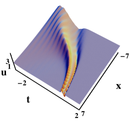
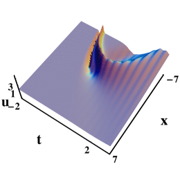
($a$)                                                                                      ($b$)

Fig.  2: Solitonic propagation and interaction with variable coefficients and spectral parameters $\overline{\lambda_{1}}=1$, $\overline{\lambda_{2}}=1.1$, $\xi_{1}=1,\xi_{2}=1$, $b(t)=1$, $c_{0}(t)=0$, $d(t)=Sin(20t)$ and line-damping coefficient: (a) $c_{1}(t)=-1$, (b) $c_{1}(t)=1$

Under the analytical discussion before, soliton amplitude can be interpreted by the effect of line-damping coefficient $d(t)$ when $\overline{\lambda}$ is given. As demonstrated in Fig. Solitons and breathers for nonisospectral mKdV equation with Darboux transformation, a periodic value independent to time is applied for $d(t)$ and correspondingly the soliton dynamics presents amplitude periodicity. Coefficient $c_{1}(t)$ is capable of describing nonuniformity of media and should be evaluated in the nonisospectral problems. For positive and negative implication of $c_{1}(t)$, the solitons propagation dynamics differs in terms of its width. With $c_{1}(t)$ being 1 and -1 in this case, the soliton compress and swell respectively along the propagation.

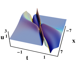
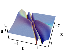
($a$)                                                                                    ($b$)

($c$)                                                                                    ($d$)

Fig.  3: Interaction among elevation and depression with variable coefficients and spectral parameters $b(t)=1$, $c_{1}(t)=t$, $c_{0}(t)=0$, $d(t)=0$, $\xi_{1}=\xi_{2}=\xi_{3}=0$, $\overline{\lambda_{1}}=1$, and $\overline{\lambda_{2}}=1.1$, (a) $\overline{\lambda_{3}}=1.5$, (b) $\overline{\lambda_{3}}=-1.5$. (c) and (d) profile (a) and (b) respectively when t=-1(solid line) and t=1(dash line)

Fig. Solitons and breathers for nonisospectral mKdV equation with Darboux transformation depicts three soliton solution, including the interaction among depression and elevation. Comparing Fig. Solitons and breathers for nonisospectral mKdV equation with Darboux transformation(a) with (b), in addition to change the value of initial phase, we could also manage to replace the elevation by depression via a sign reversal of spectral parameter $\overline{\lambda_{2}}$ from positive to negative. The three soliton propagation is exhibited by profiles in Figs. Solitons and breathers for nonisospectral mKdV equation with Darboux transformation(c) and (d) at certain time, with high-amplitude elevation (depression) firstly leaving behind the low-amplitude elevation (depression) and then surpassing when time is approaching to 1. Such phenomena are also indicated in ref [11] with Eq. (1) under an extra ($c_{1}(t)=d(t)$).

VI. Breathers and breather-soliton solutions

Breather solutions can be constructed by DT under a pair of complex conjugate spectral parameters ($\overline{\lambda_{1}}=\alpha+i\beta,\overline{\lambda_{2}}=\alpha-i\beta$). Similar to the definition that breather can be regarded as a central valley with two small hills of elevation adjacently, which should reverse its polarities every half a cycle later [21], the breather generated by DT can be also regarded as valley-hill feature in symmetric form at certain time.

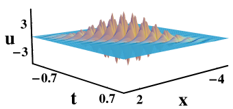
($a$)                                                                                  ($b$)

Fig.  4: (a) Breather propagation $\overline{\lambda_{1}}=1.5-i$, $\overline{\lambda_{2}}=1.5+i$, $\xi_{1}=\xi_{2}=1$, $b(t)=1$, $c_{0}(t)=c_{1}(t)=0$ and $d(t)=10\,t$; (b) Profiles (a) when t=-0.566(solid line), t=-0.267(bold dashed line), t=0.155(bold solid line) and t=0.454(dashed line)

As illustrated in Fig. Solitons and breathers for nonisospectral mKdV equation with Darboux transformation, the propagation of breathers demonstrates periodically pulsating and isolated wave forms by profiles at certain time. Fig. Solitons and breathers for nonisospectral mKdV equation with Darboux transformation(b) illustrates a downward displacement at center and the horizontal symmetry of breather structure. With line-damping coefficient $d(t)$ taken into consideration, breather propagation presents a character of time-space locality.

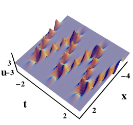
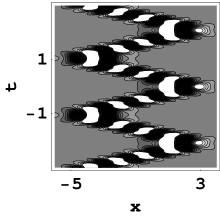
($a$)                                                                                      ($b$)

Fig.  5: (a) Breather propagation with spectral parameters $\overline{\lambda_{1}}=1-i$, $\overline{\lambda_{2}}=1+i$, initial phases $\xi_{0}=\xi_{1}=1$ and coefficients $b(t)=Sin(3t)$, $c_{0}(t)=c_{1}(t)=0$ and $d(t)=Sin(10t)$; (b) Contour plot of (a)

Fig. Solitons and breathers for nonisospectral mKdV equation with Darboux transformation shows a kind of periodic soliton solution for the existence of two periodic coefficient $b(t)=Sin(3t)$ and $d(t)=Sin(10t)$ supporting the periodically oscillating breather. From the analytical discussion, the character line is determined only by $b(t)$ when the other coefficients and parameters are given, and the time dependent $d(t)$ gives rise to the periodical soliton amplitude. In a conclusion, there exist three kinds of periodism with respect to breather, character line and the soliton amplitude.

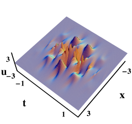
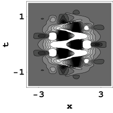
($a$)                                                                                      ($b$)

Fig.  6: (a) Interaction between a breather and a soliton $\overline{\lambda_{1}}=1-i$, $\overline{\lambda_{2}}=1+i$, $\overline{\lambda_{3}}=1$, $\xi_{1}=\xi_{2}=\xi_{3}=0$, $b(t)=sin(10t)$, $c_{0}(t)=c_{1}(t)=0$ and $d(t)=5\,t$, (b) Contour plot of (a)

The contour plot in Fig. Solitons and breathers for nonisospectral mKdV equation with Darboux transformation (b) exhibits the effects of the dispersive term $b(t)$ and line-damping term $d(t)$ on the interaction between a breather and a elevation. Being interacted by breather propagation, the elevation undergoes a similar periodicity corresponding to the breather and propagate without interrupting the pecks of breather.

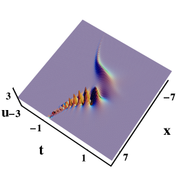
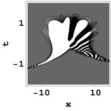
($a$)                                                                                      ($b$)

Fig.  7: (a) Interaction between a breather and a soliton $\overline{\lambda_{1}}=1-i$, $\overline{\lambda_{2}}=1+i$, $\overline{\lambda_{3}}=1$, $\xi_{1}=\xi_{2}=\xi_{3}=0$, $b(t)=1$, $c_{0}(t)=0$, $c_{1}(t)=1$ and $d(t)=10\,t$; (b) Contour plot of (a)

Fig. Solitons and breathers for nonisospectral mKdV equation with Darboux transformation depicts the collision between a soliton and breather with approximately x=0 being the intersection point, which witnesses the mutual interaction. The character line is overlapped and swell phenomena occur corresponding to the soliton and breather width. Compared with Fig. Solitons and breathers for nonisospectral mKdV equation with Darboux transformation, without periodical time-varying function $b(t)$, Fig. Solitons and breathers for nonisospectral mKdV equation with Darboux transformation demonstrates another kind of character line.

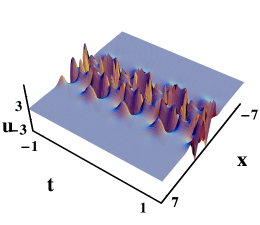
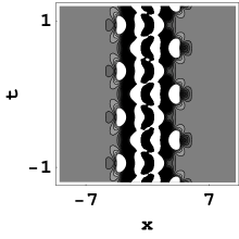
($a$)                                                                                      ($b$)

Fig.  8: (a) Interaction between two breather with spectral parameters $\overline{\lambda_{1}}=1-i$, $\overline{\lambda_{2}}=1+i$, $\overline{\lambda_{3}}=1.2-i$, $\overline{\lambda_{4}}=1.2+i$ and $\xi_{1}=\xi_{2}=\xi_{3}=0$ and coefficients $b(t)=sin(10t)$, $c_{0}(t)=c_{1}(t)=0$ and $d(t)=5Sin(10t)$; (b) Contour plot of (a)

With b(t) being periodical, we can observe two-breather periodical oscillation in Fig. Solitons and breathers for nonisospectral mKdV equation with Darboux transformation. The continuous interaction between two breathers in one period is demonstrated in the contour plot, which indicates the two-breather structure in this case can be regarded as a coherent structure.

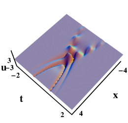
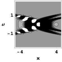
($a$)                                                                                      ($b$)

Fig.  9: (a) Interaction between a breather and two solitons with spectral parameters $\overline{\lambda_{1}}=1-i$, $\overline{\lambda_{2}}=1+i$, $\overline{\lambda_{3}}=1.2$, $\overline{\lambda_{4}}=-2$ and $\xi_{1}=\xi_{2}=\xi_{3}=\xi_{4}=0$ and coefficients $b(t)=t$, $c_{0}(t)=c_{1}(t)=0$ and $d(t)=5t$; (b) Contour plot of (a)

Fig. Solitons and breathers for nonisospectral mKdV equation with Darboux transformation illustrates the interaction between a breather and two solitons. It is worth noting that with the breather-soliton convergence at time approaching to zero, soliton amplitude also reaches its peak value due to the line-damping term $d(t)$. Compared with the structure including a soliton and a breather in Figs. Solitons and breathers for nonisospectral mKdV equation with Darboux transformation and Solitons and breathers for nonisospectral mKdV equation with Darboux transformation, Fig. Solitons and breathers for nonisospectral mKdV equation with Darboux transformation presents three character lines, which individually support two solitons and a breather in its propagation.

VII. Conclusions

Based on the introduced constraint (2), under which Eq. (1) is integrable and $c_{1}(t)$ becomes independent from $d(t)$, the work of our paper can be concluded as following:

(1) The Lax pair is generated by means of AKNS process with a nonisospectral flow under constraint (2). Meanwhile, DT is constructed based on the Lax pair, by which multi-soliton and breather solutions could be iterated from the seed ones.

(2) Analytical discussion corresponding to the characteristic line is applied, in which the one soliton amplitude (polarity), width (wave number) and velocity can be obtained. Meanwhile, with the aid of one soliton solution, multi-soliton solutions are generated with their graphical illustration. Initial phases are discussed by employing a value shift, which gives rise to the soliton inverse polarity. With appropriate selection of coefficients and spectral parameters, such reverse polarity might prevent soliton cross. In addition, variable coefficients influencing soliton amplitude, velocity and width are investigated and the interaction among three solitons is demonstrated.

(3) N-th iteration by DT can generate N-soliton solutions, including the breathers in the periodically pulsating and isolated wave forms, which are generated by employing a pair of complex conjugate spectral parameters ($\overline{\lambda_{1}}=\alpha+i\beta,\overline{\lambda_{2}}=\alpha-i\beta$) during iteration. For example, the four-soliton solution can generate two breathers with periodical oscillation as shown in Fig. Solitons and breathers for nonisospectral mKdV equation with Darboux transformation or a breather and two solitons with three character lines as shown in Fig. Solitons and breathers for nonisospectral mKdV equation with Darboux transformation. The inherent periodism of breathers and the variable coefficients of Eq. (1) have coupling effects, which can yield abundant structures of breather and soliton solutions, such as a cyclical breather of three kinds of periodism, a breather-soliton interaction with time-space locality and two-breathers in a coherent structure. Such results can be extended to multi-soliton solutions by DT and similar phenomena could be observed.

Acknowledgements

We express our sincere thanks to all the members of our discussion group for their valuable comments. This work has been supported by the National Natural Science Foundation of China under Grant No. 11302014, and by the Fundamental Research Funds for the Central Universities under Grant Nos. 50100002013105026 and 50100002015105032 (Beijing University of Aeronautics and Astronautics).

References

- [1] Z. T. Fu, S. D. Liu and S. K. Liu, Phys. Lett. A 326, 364, 2004.
- [2] Y. L. Wang, Z. X. Zhou, X. Q. Jiang, X. D. Ni, Y. Zhang, J. Shen and P. Qian, Phys. Lett. A 373, 2944, 2009.
- [3] K. Helfrich, W. K. Melville and J. W. Miles, J. Fluid. Mech. 149, 305, 1984.
- [4] D. K. Ghosh, G. Mandal, P. Chatterjee and U. N. Ghosh, IEEE Trans. Plas. Sci. 41, 5, 2013.
- [5] H. Leblond, H. Triki, F. Sanchez and D. Mihalache, Opt. Commun. 285, 356, 2012.
- [6] R. Grimshaw, D. Pelinovsky, E. Pelinovsky and T. Talipova, Phys. D 159, 35, 2001.
- [7] Y. Zhang, Z. L. Cheng and X. H. Hao, Chin. Phys. B 21, 12, 2012.
- [8] O. Vaneeva, Commun. Nonlinear Sci. Numer. Simulat. 17, 611, 2014.
- [9] X. L. Gai, Y. T. Gao, L. Wang, D. X. Meng, X. L, Z. Y. Sun and X. Yu, Commun. Nonlinear Sci. Numer. Simulat. 16, 1776, 2011.
- [10] D. E. Pelinovsky and R. H. J. Grimshaw, Phys. Lett. A 229, 165, 1997.
- [11] Z. Y. Sun, Y. T. Gao, Y. Liu and X. Yu, Phys. Rev. E 84, 026606, 2011.
- [12] C. J. Wang, Z. D. Dai, S. Q. Lin and G. Mu, Appl. Math. Comput. 216, 341, 2010.
- [13] Y. Zhang, J. B. Li and Y. N. Lv, Ann. Phys. 323, 3059, 2008.
- [14] H. C. Hu and Q. P. Liu, Chaos Solitons Fractals 17, 921, 2013.
- [15] Q. L. Zha, Commun. Nonlinear Sci. Numer. Simulat 57, 083506, 2016.
- [16] Q. L. Zha and Z. B. Li, Chin. Phys. Lett. 25, 8, 2008.
- [17] L. Wang, Y. T. Gao and F. H. Qi, Ann. Phys. 327, 1974, 2012.
- [18] X. L. Gai, Y. T. Gao, D. X. Meng, L. Wang, Z. Y. Sun, X. L, Q. Feng, M. Z. Wang, X. Yu and S. H. Zhu, Commun. Theor. Phys. 53, 673, 2010.
- [19] J. L. Ji and Z. N. Zhu, Commun. Nonlinear Sci. Numer. Simulat. 42, 699, 2017.
- [20] A. V. Slyunyaev, J. Exp. Theor. Phys 92, 529, 2001.
- [21] K. W. Chow, R. H. J. Grimshaw and E. Ding, Wave Motion 43, 158, 2005.
- [22] S. Clarke, R. Grimshaw, P. Miller, E. Pelinovsky and T. Talipova, Chaos 10, 383, 2000.
- [23] K. G. Lamb, O. Polukhina, T. Talipova, E. Pelinovsky, W. T. Xiao and A. Kurkin, Phys. Rev. E 75, 046306, 2007.
- [24] W. L. Chan and K. S. Li, J. Phys. A 27, 883, 1994.
- [25] W. L. Chan and X. Zhang, J. Phys. A 28, 407, 1995.
- [26] C. Q. Dai, J. M. Zhu and J. F. Zhang, Chaos Solitons Fractals 27, 881, 2006.
- [27] Q. Feng, Y. T. Gao, X. H. Meng, X. Yu, Z. Y. Sun, T. Xu and B. Tian, Int. J. Mod. Phys. B 25, 723, 2011.
- [28] S. Zhang and T. C. Xia, Phys. Lett. A 372, 1741, 2008.
- [29] Z. Y. Yan, Commun. Nonlinear Sci. Numer. Simulat. 4, 284, 1999.