Exoplanet phase curves at large phase angles. Diagnostics for extended hazy atmospheres.

Abstract

At optical wavelengths, Titan’s brightness for large Sun-Titan-observer phase angles significantly exceeds its dayside brightness. The brightening that occurs near back-illumination is due to moderately large haze particles in the moon’s extended atmosphere that forward-scatter the incident sunlight. Motivated by this phenomenon, here we investigate the forward scattering from currently known exoplanets, its diagnostics possibilities, the observational requirements to resolve it, and potential implications. An analytical expression is derived for the amount of starlight forward-scattered by an exponential atmosphere that takes into account the finite angular size of the star. We use this expression to tentatively estimate how prevalent this phenomenon may be. Based on numerical calculations that consider exoplanet visibility, we identify numerous planets with predicted out-of-transit forward scattering signals of up to tens of parts-per-million provided that aerosols of $\gtrsim$1 $\mu$m size form over an extended vertical region near the optical radius level. We propose that the interpretation of available optical phase curves should be revised to constrain the strength of this phenomenon that might provide insight into aerosol scale heights and particle sizes. For the relatively general atmospheres considered here, forward scattering reduces the transmission-only transit depth by typically less than the equivalent to a scale height. For short-period exoplanets the finite angular size of the star severely affects the amount of radiation scattered towards the observer at mid-transit.

1 Introduction

Given the limited possibilities that exist for the remote sensing of exoplanet atmospheres, it is crucial to understand the information contained in each observing technique and the synergies between them. In that setting, this work aims to show that brightness measurements at large star-planet-observer phase angles potentially inform on atmospheric properties such as the scale height and scattering properties of aerosols in the uppermost atmospheric layers. Our investigation is motivated by recent work on Saturn’s moon Titan (García Muñoz et al., 2017) showing that Titan brightens up at phase angles $\alpha$$>$150^∘ and that, when back-illuminated, it becomes brighter than in full illumination by a wavelength-dependent factor of 10–200. The presence of forward-scattering haze in Titan’s extended atmosphere is key to the occurrence of this optical phenomenon. Its prospective detection at an exoplanet will allow us to infer the occurrence of haze and, more importantly, will provide insight into its vertical distribution and particle size near the optical radius level. Figure (1) sketches the phenomenon.

The effect of forward scattering on the measured radius of transiting planets has been considered before (Brown, 2001; Hubbard et al., 2001; García Muñoz et al., 2012; De Kok & Stam, 2012; Robinson, 2017). In particular, De Kok & Stam (2012) note that it may bias the transit radius by up to a few scale heights in specific cases, and Robinson (2017) observes that the bias can be of hundreds of parts-per-million (ppm) for hot Jupiters. None of these works provide an easy way to quantitatively estimate the effect, or its connection with the stratification and size of the dominating atmospheric particles. As shown later, the finite angular size of the star as viewed from the planet limits the amount of starlight forward-scattered towards the observer during the transit, and forward scattering will affect the measured transit radius by less than a scale height in typical configurations with scattering particles of up to a few $\mu$m in size. Our treatment here differs from the above works in that we focus preferentially on orbital phases immediately before or after transit. This configuration is better suited to identify the forward scattering contribution.

To date, the best evidence for forward scattering from exoplanets comes from ultra-short period planets on orbits of less than one day. In a few such systems, the shape of the pre-/post-transit brightness curve is attributed to starlight scattered from dust clouds surrounding the planets (e.g. Budaj, 2013; DeVore et al., 2016). Since the dust is plausibly of planetary origin, these planets are thought to be disintegrating. Refraction may also produce shoulders in the pre-/post-transit brightness curve (Hui & Seager, 2002; Sidis & Sari, 2010; García Muñoz & Mills, 2012; García Muñoz et al., 2012; Misra & Meadows, 2014). Refraction lensing of starlight by the planet atmosphere competes with extinction within the atmosphere. As a result, a brightness surge due to refraction will be prominent only on planets with clear, aerosol-free envelopes (García Muñoz & Mills, 2012; Misra & Meadows, 2014). Contrary to forward scattering, refraction lensing becomes significant for planets on relatively long-period orbits (Sidis & Sari, 2010; Misra & Meadows, 2014). This distinction should make it posible to identify whether the brightness surge is due to refraction or to forward scattering.

The paper is structured as follows. In §2 we summarize the findings on Titan that motivate this study and generalize them for application to exponential atmospheres. In §3 we describe, through combined analytical and numerical work, the planet properties more favourable for forward scattering. Based on a zeroth-order characterization, we attempt to classify the known exoplanets according to their potential for forward scattering. In §4 we elaborate further on the detectability of this phenomenon out of transit. In §5 we comment on the blending with the brightness modulation due to stellar tides, and on the impact upon the measured transit radius. Finally, §6 summarizes the main conclusions and presents avenues for follow-up studies. In the appendices, we derive an analytical expression for the amount of starlight forward scattered by a planet with an exponential atmosphere, comment on the accuracy of the single scattering approximation, and describe the modifications to our numerical radiative transfer model to take into account the finite angular size of the star.

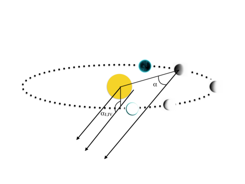
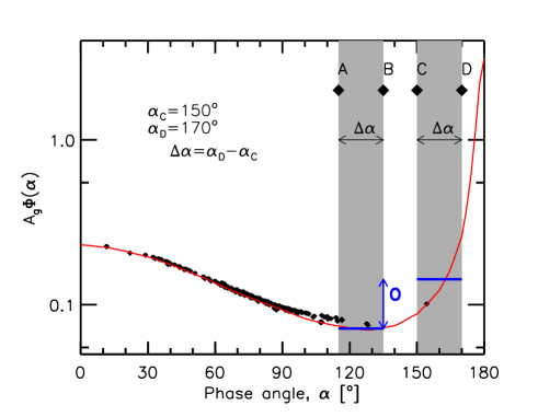
Figure 1: Top. Orbit sketch. $\alpha$ is the star-planet-observer phase angle and $\alpha_{\rm{I,IV}}$ the angle at first or fourth contacts, i.e. immediately before or after transit. The arrows indicate the direction towards the observer. Bottom. Titan’s phase curve from Cassini/ISS white-light photometry (effective wavelength of 650 nm) (black symbols) and best-fit model based on solving the radiative transfer problem with a realistic description of the atmosphere (red curve) (García Muñoz et al., 2017). The two grey intervals span an identical range $\Delta\alpha$ of phase angles, and indicate the forward scattering and control intervals (see text). The observable O is defined as the difference in the mean values of the planet brightness over the two intervals. In the example, $\alpha_{\rm{D}}$=170^∘ and $\Delta\alpha$=20^∘. In the examples with real planets, we always assume $\alpha_{\rm{D}}$=$\alpha_{\rm{I,IV}}$.

2 Forward scattering

2.1 Titan

The brightness phase curve of Titan is quite unique. Titan dims as it passes from phase angles $\alpha$=0 to $\alpha$$\sim$120^∘ due to the decreasing area of the dayside visible to the observer (Tomasko & Smith, 1982; West et al., 1983). For larger phase angles, however, the diminishing size of the visible dayside is compensated by forward scattering from the abundant upper-atmosphere haze and the whole-disk brightness increases again. Observations made with the Cassini Imaging Science Subsystem have revealed that at $\alpha$$\sim$165^∘ Titan becomes as bright as in full illumination (García Muñoz et al., 2017). An empirically-constrained prediction of that study is that for $\alpha$$\rightarrow$180^∘, Titan’s twilight appears brighter than its dayside by a factor of $\sim$10 at wavelengths of $\sim$1 $\mu$m and by factors of up to 200 at wavelengths of $\sim$300 nm.

This behaviour is due to the facts that Titan has an atmosphere that is both extended and hazy, and that the haze particles are moderately large (equal-projected-area radii $\sim$2–3 $\mu$m) and thus efficient at forward scattering (Rages et al., 1983; West & Smith, 1991). The haze is produced photochemically through reactions initiated in the upper atmosphere (Lavvas et al., 2010). Forward scattering from Titan originates within a few scale heights from the level at which the atmosphere is optically thick when viewed through the limb. This is similar to the optical radius level probed during a hypothetical transit of Titan across the solar disk (Karkoschka et al., 1997; Lecavelier des Etangs et al., 2008). Near that level, the number densities of the gas and haze drop in altitude with comparable scale heights, $H$$\sim$$H_{\rm{a}}$$\sim$45 km. If $R_{\rm{T}}$ stands for Titan’s optical radius ($\sim$3,000 km, dependent on wavelength), $H_{\rm{a}}$/$R_{\rm{T}}$$\sim$1.5$\times$10^-2.

2.2 Exponential atmospheres

Next, we identify the key planet properties that result in strong forward scattering. Appendix A elaborates on exponential atmospheres described in terms of an average scattering particle and a single scale height. We will refer to the average scattering particles as aerosols, although they may actually represent a mix of gases and condensates in the atmosphere. For an exponential atmosphere, the aerosol number density decays as $n_{\rm{a}}$($r$)=$n_{\rm{a}}$($R_{\rm{0}}$)$\exp{(-(r-R_{\rm{0}})/H_{\rm{a}})}$, where $r$ is the radial distance to the planet centre and $R_{\rm{0}}$ is a reference level. $H_{\rm{a}}$ is the aerosol scale height.

In this idealized scenario and $\alpha$$\rightarrow$180^∘, single scattering dominates (Appendix B) and the planet-to-star contrast is approximately (Appendix A):

$$\frac{F_{\rm{p}}}{F_{\star}}(\alpha=180^{\circ})\approx\underbrace{2\pi p_{\rm{a}}(\theta=0)\varpi_{0,\rm{a}}\frac{H_{\rm{a}}}{R_{\rm{p}}}}\left(\frac{R_{\rm{p}}}{a}\right)^{2}.$$ (1)

Here, $p_{\rm{a}}$$(\theta$=0) and $\varpi_{0,\rm{a}}$ refer to the aerosol scattering phase function in the forward direction (scattering angle $\theta$=0) and the aerosol single scattering albedo, respectively. ($p_{\rm{a}}$$(\theta$=0) is the relevant phase function when the angular size of the star as viewed from the planet is small, i.e. in the point-like star limit; otherwise a generalized form $\mbox{<}p_{\rm{a}}\mbox{>}$$(\Theta$=0) should be used, Appendix A.) $H_{\rm{a}}$/$R_{\rm{p}}$ is the ratio of the aerosol scale height to the planet radius, and $R_{\rm{p}}$/$a$ the ratio of the planet radius to the orbital distance. The geometrical terms in Eq. (1) can be re-arranged into 2$\pi$$R_{\rm{p}}$$H_{\rm{a}}$/$a^{2}$, the numerator of which is the projected area of a ring of radius $R_{\rm{p}}$ and width $H_{\rm{a}}$. This ring, which concentrates most of the forward-scattered starlight, is seen in large phase angle images of Titan (García Muñoz et al., 2017). Equation (1) is analogous to the usual representation of the planet-to-star brightness contrast in full illumination ($\alpha$=0) if the underlined terms are replaced by the geometric albedo, $A_{\rm{g}}$ (see Eq. 2 below). Equation (1) enables the direct comparison of the brightness of a planet when it is fully illuminated ($\alpha$=0) and back-illuminated ($\alpha$=180^∘).

The single scattering albedo $\varpi_{0,\rm{a}}$ is of order one for many plausible condensates in exoplanet atmospheres (Budaj et al., 2015; Wakeford & Sing, 2015). However, both $p_{\rm{a}}$$(\theta$=0) and $H_{\rm{a}}$/$R_{\rm{p}}$ are likely to differ by orders of magnitude amongst different planets depending on the specifics of their atmospheres. (However, for short-period planets the finite angular size of the star will limit the effective scattering phase function to $\mbox{<}p_{\rm{a}}\mbox{>}$$(\Theta$=0), which may be much smaller than $p_{\rm{a}}$$(\theta$=0); Appendix A.) $H_{\rm{a}}$/$R_{\rm{p}}$ is a measure of how puffy the atmosphere is, meaning that large ($\sim$10^-2) values are associated with extended envelopes. It is seen from Eq. (1) that for a given $R_{\rm{p}}$/$a$ (measurable for transiting systems), the strength of forward scattering depends on $p_{\rm{a}}$$(\theta$=0)$H_{\rm{a}}$/$R_{\rm{p}}$. Also according to Eq. (1), the strength of this effect depends on orbital distance as $a^{-2}$. This interpretation is however likely oversimplistic as the orbital distance will foreseeably affect the planet temperature and therefore $p_{\rm{a}}$($\theta$) through the microphysics that enables aerosol formation. Also, for small orbital distances, the finite size of the star tends to reduce the relevant $\mbox{<}p_{\rm{a}}\mbox{>}$$(\Theta$=0) with respect to $p_{\rm{a}}$$(\theta$=0).

To illustrate how forward scattering affects the planet brightness at configurations other than $\alpha$=180^∘, we produced numerical solutions to the problem of multiple scattering in spherical, exponential atmospheres. We generally assumed that the aerosols scatter following Mie theory, and that the photon wavelength is $\lambda_{\rm{eff}}$=0.65 $\mu$m. For the aerosol particles we assumed a power law size distribution with effective radii $r_{\rm{eff}}$ ranging from 0.01 to 10 $\mu$m and a fixed effective variance $v_{\rm{eff}}$=0.1 (Hansen & Travis, 1974). We adopted refractive indices ($n$=$n_{\rm{r}}$+i$n_{\rm{i}}$) specific to a few plausible condensates listed in Table (1). The selection of condensates does not rank them by relevance in the context of exoplanet atmospheres. Rather, it simply tries to include a variety of refractive indices. In Mie theory, $p_{\rm{a}}$($\theta$) depends on all three properties: $x_{\rm{eff}}$=2$\pi$$r_{\rm{eff}}$/$\lambda_{\rm{eff}}$, $v_{\rm{eff}}$ and $n$. More specifically, $p_{\rm{a}}$($\theta$=0) depends strongly on $x_{\rm{eff}}$ but weakly on $v_{\rm{eff}}$ and $n$, and typically increases as $x_{\rm{eff}}$ increases, which establishes a diagnostic connection between the particle size and the strength of forward scattering. The implemented single scattering albedos $\varpi_{0,\rm{a}}$ were also calculated from Mie theory. Figure (2) shows the calculated $p_{\rm{a}}$($\theta$=0) and $\varpi_{0,\rm{a}}$. For comparison, we also produced phase curves based on atmospheres with Titan-like haze at an effective wavelength $\lambda_{\rm{eff}}$=600 nm. In these cases, we adopted $p_{\rm{a}}$($\theta$) as reported in Table 1 of Tomasko et al. (2008), and for $\varpi_{0,\rm{a}}$ we simply experimented with values between 0.2 and 1.

Table 1: Refractive indices of condensates at $\lambda_{\rm{eff}}$=0.65 $\mu$m, based on Budaj et al. (2015) and Wakeford & Sing (2015). (The latter quote condensation temperatures at 1 mbar pressure.) Note: DOCDD: http://www.astro.uni-jena.de/Laboratory/OCDB/. For the calculation of optical properties, we used Mie theory (www.giss.nasa.gov/staff/mmishchenko/t$\_$matrix.htmlS).

Composition	$n_{\rm{r}}$	$n_{\rm{i}}$	Ref.
SiO2	1.5	10-7	see García Muñoz & Isaak (2015)
Al2O3	1.56	1.3$\times$10-2	Koike et al. (1995)
FeO	2.42	0.60	DOCDD
CaTiO3	2.25	10-4	see García Muñoz & Isaak (2015)
Fe2O3	2.84	0.23	DOCDD
Fe2SiO4	1.85	7.7$\times$10-4	DOCDD
Mg2SiO4//MgSiO3	1.6	10-4	see García Muñoz & Isaak (2015)
TiO2	2.57	1.8$\times$10-4	DOCDD
Fe	2.92	3.10	Johnson & Christy (1974)
C	1.59	0.73	DOCDD

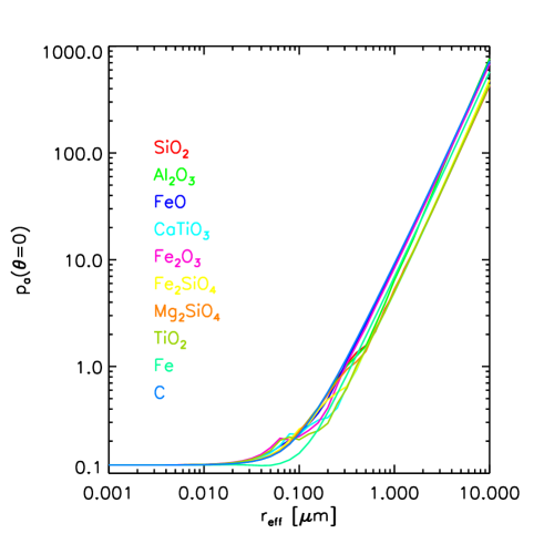
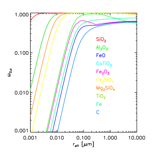
Figure 2: Top. Scattering phase function in forward scattering $p_{\rm{a}}$($\theta$=0) for the condensates of Table (1). (The finite angular size of the star reduces the effective scattering phase function $<$$p_{\rm{a}}$($\Theta$=0)$>$ with respect to $p_{\rm{a}}$($\theta$=0); see Fig. (11).) We normalize $p_{\rm{a}}$($\theta$) so that its integral over 4$\pi$ is equal to one (Appendix A). Bottom. For the same condensates, their corresponding single scattering albedo, $\varpi_{\rm{0,a}}$.

For the smaller orbital distances, the star appears as an extended object as viewed from the planet, a fact that must be considered in the implementation of the aerosols scattering phase function going into the multiple scattering calculations. The way to deal with this is to convolve $p_{\rm{a}}$($\theta$) with the star disk brightness (Budaj et al., 2015; DeVore et al., 2016) in the evaluation of the starlight entering the atmosphere (§4.1, and Appendices A and C). The resulting effective scattering phase function $\mbox{<}p_{\rm{a}}\mbox{>}$($\Theta$) depends on the limb-darkening law and the angular size of the star. For $p_{\rm{a}}$($\theta$) functions associated with strong forward scattering, the effective scattering phase function for deflections larger than the angular radius of the star, i.e. $\Theta$$>$$\theta_{\star}$$=$$\arcsin{R_{\star}/a}$, is usually larger than the non-convolved $p_{\rm{a}}$($\theta$) (Fig. 3, Budaj et al. (2015); Fig. 11 in Appendix A). The opposite is generally true for $\Theta$$<$$\theta_{\star}$. In contrast, for $p_{\rm{a}}$($\theta$) functions associated with mild forward scattering, the convolution process has little impact on the effective scattering phase function $\mbox{<}p_{\rm{a}}\mbox{>}$($\Theta$) (Fig. 3, Budaj et al. (2015); Figs. 3 and A2, DeVore et al. (2016)). For simplicity, as the convolution process is specific to each planet-star system, we have omitted this effect from most of the multiple scattering calculations done here. Its omission will tend to increase the forward scattering signal towards the observer at out-of-transit orbital phases. Therefore, the calculations presented here in the point-like star limit for pre-/post-transit configurations generally underestimate the actual forward scattering signal received by the observer. In §4.1, we provide examples of how the finite angular size of the star will impact the brightness phase curve in the specific case of the exoplanet CoRoT-24b.

It is convenient to present the planet-to-star contrast in a manner that separates the various geometric and non-geometric factors:

$$\frac{F_{\rm{p}}}{F_{\star}}(\alpha)=A_{\rm{g}}\Phi(\alpha)\left(\frac{R_{\rm{p}}}{a}\right)^{2}.$$ (2)

Here, $A_{\rm{g}}$ is the geometric albedo and $\Phi$($\alpha$) ($\Phi$($\alpha$$\equiv$0)=1) the planet phase law. The definition of $R_{\rm{p}}$ is somewhat arbitrary for planets with extended atmospheres. Because we are mainly interested in gas planets with large scale heights, we will use for $R_{\rm{p}}$ the optical radius, which is based on the limb-viewing optical thickness of the atmosphere, $\tau_{\rm{limb}}$. The optical radius at an effective wavelength $\lambda_{\rm{eff}}$ is calculated from the condition (Karkoschka et al., 1997; Lecavelier des Etangs et al., 2008):

$$\tau_{\rm{limb}}(R_{\rm{p}})=\tau_{\rm{nadir}}(R_{\rm{p}}\rightarrow{\rm{TOA}})(2\pi R_{\rm{p}}/H_{\rm{a}})^{1/2}=0.56,$$ (3)

and the optical thickness from the optical radius level $R_{\rm{p}}$ to the top of the atmosphere (TOA):

$$\tau_{\rm{nadir}}(R_{\rm{p}}\rightarrow{\rm{TOA}})=\tau_{\rm{nadir},0}\exp{(-(R_{\rm{p}}-R_{\rm{0}})/H_{\rm{a}})}.$$ (4)

The square root term in Eq. (3) is the approximate conversion factor between limb- and nadir-integrated columns in exponential atmospheres. $\tau_{\rm{nadir},0}$ is the nadir optical thickness upwards of the $R_{\rm{0}}$ reference level. We could take $R_{\rm{0}}$ deep enough into the planet and $\tau_{\rm{nadir},0}$ large enough so that the exponential description of the atmosphere effectively reaches to all depths. Instead, and to alleviate the computational cost of the calculations, we implemented finite values for $R_{\rm{0}}$ (equal to a Jupiter radius, $R_{\rm{J}}$) and $\tau_{\rm{nadir},0}$ (=10). Also, the atmosphere below the $R_{\rm{0}}$ level was replaced by a black surface. The truncation of the atmosphere at $R_{\rm{0}}$ will affect the planet’s overall reflectance at the smaller phase angles, but not at large phase angles because in the latter viewing configuration the stellar photons will not penetrate to such depths. $R_{\rm{p}}$ ($>$$R_{\rm{0}}$) can be solved numerically from Eqs. (3)–(4) for a given scale height $H_{\rm{a}}$.

In total, we produced about 800 phase curves for different combinations of aerosol composition, particle radius and ratio of the aerosol scale height to the planet optical radius. Figure (3) shows a subset of them in the dimensionless form $A_{g}$$\Phi(\alpha)$. From top to bottom, the graphs are arranged by increasing $H_{\rm{a}}$/$R_{\rm{p}}$. It is apparent that puffy planets with large $H_{\rm{a}}$/$R_{\rm{p}}$ ratios exhibit stronger forward scattering. $A_{g}$$\Phi(\alpha)$$>$1 is possible at large phase angles, especially for puffy atmospheres rich in large aerosol particles. This physically consistent result confirms that the overall planet brightness mimics to some extent the behaviour of the aerosols scattering phase function when the planet is back-illuminated.

The graphs in the left and central columns show the impact of particle size for two compositions that result in more reflective (Mg₂SiO₄) or absorbing (FeO) aerosols. The effective radius of the particles $r_{\rm{eff}}$ affects both $p_{\rm{a}}(\theta)$ and $\varpi_{0,\rm{a}}$. Larger $r_{\rm{eff}}$ values typically lead to $p_{\rm{a}}$($\theta$) functions with a stronger diffraction peak focused on a narrower range of scattering angles. This behaviour is mimicked by the planet phase curve, which tends to exhibit a brightness surge closer to $\alpha$=180^∘. The finite angular size of the star, an effect omitted in the calculations of Fig. (3), will smear the forward scattering peak and leak it into smaller angles (see §4.1).

At small phase angles, the planet brightness is strongly dependent on $\varpi_{0,\rm{a}}$. The simulations show that atmospheres with Mg₂SiO₄ aerosols ($\varpi_{0,\rm{a}}$$\sim$0.997 for $r_{\rm{eff}}$=1 $\mu$m) result in brighter planets than if they are rich in FeO aerosols ($\varpi_{0,\rm{a}}$$\sim$0.555 for $r_{\rm{eff}}$=1 $\mu$m). At large phase angles however the dependence of the planet brightness with the assumed $\varpi_{0,\rm{a}}$ is almost linear (Eq. 1) and the difference between the Mg₂SiO₄- and FeO-aerosol atmospheres is reduced.

The graphs in the right column of Fig. (3) show phase curves calculated with Titan-like haze scattering phase functions $p_{\rm{a}}$($\theta$) at $\lambda_{\rm{eff}}$=600 nm (Tomasko et al., 2008). To explore the impact of $\varpi_{0,\rm{a}}$, we ran this set of simulations with $\varpi_{0,\rm{a}}$ values between 0.2 and 1, as indicated in the graphs. This battery of simulations confirms that the planet brightness is very sensitive to $\varpi_{0,\rm{a}}$ at the small phase angles, but much less so at large phase angles.

As a corollary, the analytical expression of Eq. (1) (and its generalization to finite angular size stars) together with the phase curves of Fig. (3) indicate that: extended hazy atmospheres result in significant forward scattering at large phase angles; the aerosol size partly dictates the strength of the phenomenon and whether it occurs on either a narrow or broad range of phase angles (at least in the point-like star limit); the aerosol composition is not critical at large phase angles. The arguments presented above suggest that the detection of such an optical phenomenon at an exoplanet will lead to a joint constraint on its aerosol scale height and particle size.

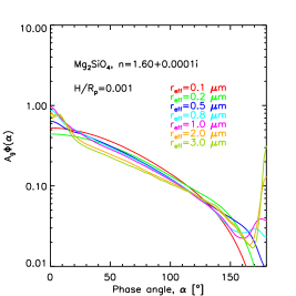
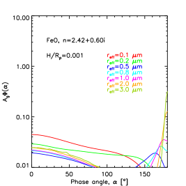
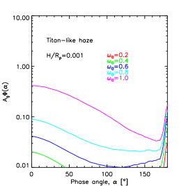
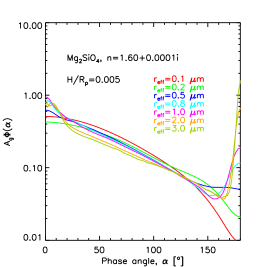
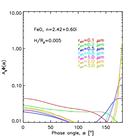
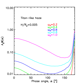
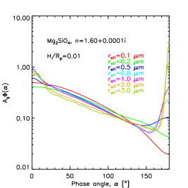
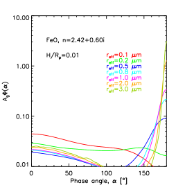
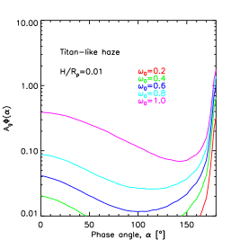
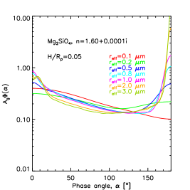
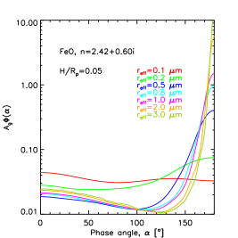
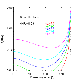
Figure 3: Reflected starlight phase curves for spherical, exponential atmospheres. Three types of scattering aerosols are considered: Mg₂SiO₄ (left), FeO (middle) and Titan-like haze (right). From top to bottom, the graphs explore increasing values of $H_{\rm{a}}$/$R_{\rm{p}}$. The phase curves are normalized as in Eq. (2), with $R_{\rm{p}}$ being the optical radius. The simulations are based on the point-like star limit, thereby assuming that the angular size of the star is small. A non-negligible angular size will modify the phase curves by leaking some of the forward-scattered radiation to smaller phase angles (see §4.1).

3 Extended hazy atmospheres

Diverse theoretical approaches to the formation of condensates in exoplanet atmospheres of different complexity and scope have been presented in the literature (e.g. Marley et al., 1999; Sudarsky et al., 2000; Ackerman & Marley, 2001; Morley et al., 2012; Helling & Fomins, 2013; Parmentier et al., 2013; Lee et al., 2016; Lavvas & Koskinen, 2017). Their predictive capacity however remains uncertain. In an attempt to develop a few guidelines, Sudarsky et al. (2000) proposed five broadly-defined regimes in the formation of condensates on substellar gas objects depending on the objects temperature. This classification is not comprehensive, but is useful because reveals part of the complexity of the problem. Specifically, the authors indicate that the low-gravity ($g$$<$10 m s^-2), very hot ($>$1,500 K) planets of their Class V are likely to have silicate condensates lofted high in their (extended) atmospheres and therefore appear as highly reflective during occultations and hazy during transits. If the prediction is correct, these planets would be potential candidates for strong forward scattering provided that the condensate particles are of the appropriate size.

The increasing number of exoplanet data has also led to phenomenological approaches that seek to correlate the empirical evidence for condensates with properties such as planet gravity or temperature (Stevenson, 2016), water absorption (Sing et al., 2016), or the muting of alkali features in the visible and near infrared (Heng, 2016). In particular, Stevenson (2016) suggests on the basis of near-infrared observations for 14 exoplanets that condensates form preferentially in low gravity ($g$$<$16 ms^-2), low temperature ($T_{\rm{eq}}$$<$750 K) environments. On the other hand, Barstow et al. (2017) note that from their sample of 10 hot Jupiters the planets with $T_{\rm{eq}}$$<$1,300 or $>$1,700 K seem to exhibit Rayleigh extinction at short wavelengths attributable to small condensates. In contrast, the planets of their sample with temperatures in the 1,300–1,700 K range seem to exhibit wavelength-independent extinction suggestive of larger condensates. The predictive capacity of phenomenological approaches remains to be confirmed with additional targets and tested with robust interpretation tools (Stevenson et al., 2016).

The uncertainties in the occurrence of condensates in exoplanet atmospheres translate into uncertainties in their vertical distribution, composition and particle size. Sing et al. (2016) note that if the pressure-temperature profile of an atmosphere runs (nearly) parallel to the condensation curve of a potential condensate, disturbances in the temperature-pressure profile may cause that the planet atmosphere shows itself as either hazy or essentially clear. The condensate composition will depend on the material available for condensation and on the local chemistry if the haze is formed photochemically. The particle size will depend on these effects, but also on competing microphysical processes that may either favour or disrupt the growth of small aerosols onto larger ones. Atmospheric dynamics, and its capacity to keep the particles suspended against gravitational settling, will also play a role.

A number of exoplanets reveal continuum extinction that increases towards ultraviolet wavelengths. The usual interpretation of this behaviour is that the wavelength-dependent extinction cross sections of small, weakly-absorbing particles ($\sigma$$\propto$$\lambda^{-\alpha}$ with $\alpha$$\sim$4) cause the so-called Rayleigh slopes in the planet transmission spectra (Lecavelier des Etangs et al., 2008). Evidence for small condensates has also been found in the interpretation of reflected starlight. Planets with large-particle clouds will likely exhibit more structure in their brightness variation with orbital phase than if the particles are small (Seager et al., 2000; Jenkins & Doyle, 2003). This idea lies at the core of a recent analysis of Kepler-7b’s optical phase curve that shows that the measurements are consistent with morning-side clouds made of poorly absorbing, submicron-size particles (García Muñoz & Isaak, 2015).

Other planets show no detectable colour dependence in their transit depths. Two well-known cases of this grey behaviour are the sub-Neptunes GJ1214b (Kreidberg et al., 2014) and GJ436b (Knutson et al., 2014). In both cases, the bulk atmospheric composition is possibly dominated by hydrogen and thus they may have non-negligible scale heights. If so, grey transits are suggestive of moderately large particles lofted to mbar–$\mu$bar pressures. In spite of multiple degeneracies in the interpretation of grey transits, it is possible to constrain the location of the effective cloud level, defined as an artifical cutoff between two distinct altitude ranges: one opaque and one aerosol free. It has not been possible though to gain insight into the vertical profile of the condensates. Achieving this calls for more elaborate treatments of the aerosol vertical distribution that may not be justifiable given the multiple degeneracies already identified in the interpretation of transmission spectra. Regardless of the various uncertainties that exist in the nature of condensates and their distribution, grey transits suggest the possibility of atmospheres containing moderately large particles. If the condensates are distributed over a sufficiently broad range of altitudes, such planets might exhibit forward scattering to some extent.

The fact that some exoplanets have anomalously large radii for their age is well documented. Such inflated, low-density planets occur amongst the population of hot Jupiters (Demory & Seager, 2011) and sub-Neptunes (Lammer et al., 2016; Cubillos et al., 2017). The inflation mechanisms that sustain their interior structure have not been fully elucidated (Spiegel et al., 2014), but it is possible that there are multiple at play (Tremblin et al., 2017). Low-density exoplanets may represent good candidates for showing forward scattering provided that their extended atmospheres are accompanied by extended aerosol layers. In what follows, we derive expressions that allow us to guess when an exoplanet has suitable conditions for forward scattering. These expressions incorporate a few necessary simplifying assumptions on the envelopes.

For that purpose, we first write $H$/$R_{\rm{p}}$ in terms of measurable quantities. $H$=$kT$/$\mu g$ is the gas pressure scale height, where $k$ is the Boltzmann constant, $T$ stands for temperature, $\mu$ is the atmospheric molecular mass, and $g$ the gravitational acceleration. The relevant $H$ must be estimated near the optical radius level, which is also the level probed during transit. Since $g$=$GM_{p}$/$R_{p}^{2}$, where $G$ is the gravitational constant, and $M_{\rm{p}}$ is the planet mass, we obtain:

$$\frac{H}{R_{\rm{p}}}=\frac{kT/\mu}{GM_{\rm{p}}/R_{\rm{p}}}.$$ (5)

In our treatment we assume that the atmospheric pressure scale height and the aerosol scale height are equal, i.e. $H$=$H_{\rm{a}}$. This is very approximately the case for Titan (Tomasko et al., 2008). For other solar system planets, $H_{\rm{a}}$ is a fraction of $H$ (Sánchez-Lavega et al., 2004; Pérez-Hoyos et al., 2016), with the exact $H_{\rm{a}}$/$H$ ratio depending on the range of altitudes being considered and on whether the aerosols include the high-altitude haze that occur in most atmospheres. If the conditions in the atmosphere are such that $H_{\rm{a}}$$\ll$$H$, forward scattering will be negligible and therefore undetectable.

Measurements of temperature at the optical radius level are not available. Instead, we will use for our estimates the planet equilibrium temperature $T_{\rm{eq}}$=$T_{\rm{eff}}$($R_{\star}$/2$a$)^1/2 that assumes that the incident stellar flux (effective temperature $T_{\rm{eff}}$) is balanced by thermal radiation from a rapidly-rotating dark planet. $T_{\rm{eq}}$ does not pertain to a specific altitude and thus it is possible that the temperature at the optical radius level will differ from it.

Re-arranging Eq. (5) with the expression for $T_{\rm{eq}}$:

$$\frac{H}{R_{\rm{p}}}=4.69\times 10^{-6}\frac{T_{\rm{eq}}[{\rm{K}}]R_{\rm{p}}/R_{\rm{J}}}{{\mu[\rm{a.m.u.}}]M_{\rm{p}}/M_{\rm{J}}}=$$

$$=2.26\times 10^{-7}T_{\rm{eff}}[{\rm{K}}]\left(\frac{R_{\star}/R_{\sun}}{a[\rm{AU}]}\right)^{1/2}\frac{R_{\rm{p}}/R_{\rm{J}}}{{\mu[\rm{a.m.u.}}]M_{\rm{p}}/M_{\rm{J}}}.$$ (6)

Finally, if Eqs. (1) and (6) are combined:

$$\frac{F_{\rm{p}}}{F_{\star}}=3.23\times 10^{-13}T_{\rm{eff}}(R_{\star}/R_{\sun})^{1/2}\frac{p_{\rm{a}}(\theta=0)\varpi_{0,\rm{a}}}{\mu[\rm{a.m.u.}]\rho_{\rm{p}}/\rho_{\rm{J}}{(a[\rm{AU}])^{5/2}}},$$ (7)

where $\rho_{\rm{p}}$/$\rho_{\rm{J}}$ is the planet density relative to Jupiter’s and $R_{\star}/R_{\sun}$ is the stellar radius relative to the Sun’s. The appeal of Eq. (7) is that the information needed for its evaluation is available for many systems. It suggests that low-density planets at small orbital distances are good candidates for the occurrence of forward scattering. The reality may be more complex than that, because it is unclear how these and other parameters will affect the occurrence of aerosols and their optical properties.

In a zeroth-order approximation, the amount of forward scattering from a planet can be ranked on the basis of the planet-to-star contrast at $\alpha$=180^∘. This simplified treatment avoids elaborate calculations such as those presented in Fig. (3). According to Eq. (1), the amount of forward-scattered starlight depends on the product of 2$\pi H_{\rm{a}}/R_{\rm{p}}(R_{\rm{p}}/a)^{2}$, which is essentially a geometric factor, and $p_{\rm{a}}(\theta=0)\varpi_{0,\rm{a}}$, which depends on the aerosol optical properties (and possibly, the star angular size).

We have searched the exoplanets.org (Han et al., 2014) and exoplanetarchive.ipac.caltech.edu archives and collected the information needed in Eqs. (1), (6)–(7). As of the time of writing (April 2017), this information is available for a total of 462 exoplanets. Then, we calculated ${H}/{R_{\rm{p}}}$, $(R_{\rm{p}}/a)^{2}$, $T_{\rm{eq}}$, $\rho_{\rm{p}}$/$\rho_{\rm{J}}$, $g$/$g_{\rm{J}}$ and $2\pi(H/R_{\rm{p}})(R_{\rm{p}}/a)^{2}$. For simplicity, $a$ is taken to be the semi-major axis, also for planets on eccentric orbits. Since most planets of interest have densities consistent with hydrogen-helium envelopes, we adopted $\mu$=2.3 a.m.u. Table (2) shows a selection of the planets investigated arranged by decreasing $2\pi(H/R_{\rm{p}})(R_{\rm{p}}/a)^{2}$. Table (3) shows the same information specific to the Kepler planets discussed in Angerhausen et al. (2015) and Esteves et al. (2015).

The estimated $H$/$R_{\rm{p}}$, $(R_{\rm{p}}/a)^{2}$, $T_{\rm{eq}}$ and $2\pi(H/R_{\rm{p}})(R_{\rm{p}}/a)^{2}$ are displayed in Fig. (4). The dashed lines in Fig. (4, Top) divide the region of the parameter space with $2\pi(H/R_{\rm{p}})(R_{\rm{p}}/a)^{2}$ $>$ or $<$ 5, 10, 15, 20 and 25 parts per million (ppm). According to Eq. (1), on top of each dashed line, aerosols with $p_{\rm{a}}$($\theta$=0)$\varpi_{0,\rm{a}}$=1 (or more generally $\mbox{<}p_{\rm{a}}\mbox{>}$($\Theta$=0)$\varpi_{0,\rm{a}}$=1) will produce the quoted planet-to-star contrast at $\alpha$=180^∘. This is not an unrealistic situation, as the aerosol optical properties graphed in Fig. (2) and Fig. (11) suggest.

Table 2: Partial list of discovered exoplanets ordered by decreasing 2$\pi$$H_{\rm{a}}$$R_{\rm{p}}$/$a^{2}$. The full list is available through the journal website. The list excludes KOI-55 b and KOI-55 c, both with $T_{\rm{eq}}$$\sim$7000 K, but densities $\rho_{\rm{p}}$/$\rho_{\rm{J}}$$\sim$4.5 incompatible with hydrogen-helium envelopes. For simplicity, we assumed that the atmospheres of all planets are dominated by hydrogen-helium, although this is not necessarily the case for many of them, including the well-studied GJ1214b. The observable O has been estimated from phase curves calculated in the point-like star limit. Therefore, the quoted Os likely underestimate the starlight forward-scattered and reaching the observer. Missing fields are due to the absence of the stellar magnitude from the consulted catalogues, or because $\alpha_{\rm{D}}$$<$160^∘. The ratio (2$\pi$$H_{\rm{a}}$$R_{\rm{p}}$/$a^{2}$)/PN is an indicator of the potential forward scattering strength vs. photon noise.

Planet	$H_{\rm{a}}$/$R_{\rm{p}}$	($R_{\rm{p}}$/$a$)2	$T_{\rm{eq}}$	2$\pi$$H_{\rm{a}}$$R_{\rm{p}}$/$a^{2}$	$\rho_{\rm{p}}$/$\rho_{\rm{J}}$	$g$/$g_{\rm{J}}$	$\alpha_{\rm{D}}$	$t_{\Delta\alpha}$	$m_{V}$	PN	2$\pi$$H_{\rm{a}}$$R_{\rm{p}}$/$a^{2}$	O0.5μm	O1μm	O2μm
		[ppm]	[K]	[ppm]			[∘]	[s]		[ppm]	/PN	[ppm]	[ppm]	[ppm]
WASP-12 b	0.0070	1378.	2584.	60.6	0.24	0.42	160.7	188.	11.7	96.2	0.63	37.3	24.9	9.6
WASP-121 b	0.0076	1173.	2360.	55.9	0.18	0.34	164.7	1439.	10.4	19.6	2.85	38.5	31.2	11.6
WASP-19 b	0.0052	1576.	2066.	51.9	0.42	0.58	163.8	724.	12.6	71.8	0.72	38.4	30.1	11.1
HAT-P-65 b	0.0141	499.	1931.	44.3	0.08	0.15	167.5	4659.	13.1	37.1	1.19	29.0	27.6	11.4
WASP-103 b	0.0053	1291.	2505.	42.7	0.42	0.64	160.7	163.	12.1	123.9	0.34	28.8	19.4	7.4
WASP-76 b	0.0089	671.	2183.	37.4	0.15	0.27	166.0	2617.	9.5	9.4	3.98	26.0	22.6	8.6
HAT-P-67 b	0.0242	224.	1934.	34.1	0.04	0.08	169.6	11025.	10.1	6.0	5.71	22.0	24.7	11.9
HAT-P-32 b	0.0076	595.	1786.	28.3	0.15	0.27	170.5	5426.	11.4	15.9	1.78	22.7	28.7	14.2
WASP-78 b	0.0091	483.	2295.	27.5	0.18	0.30	163.8	1970.	12.0	33.4	0.82	17.6	13.4	5.0
CoRoT-1 b	0.0056	756.	1900.	26.7	0.31	0.46	168.3	3011.	13.6	57.2	0.47	21.6	22.9	9.5
KELT-14 b	0.0054	734.	1962.	25.1	0.24	0.42	166.5	2675.	11.0	18.2	1.38	19.6	18.2	6.9
WTS-2 b	0.0037	1072.	1544.	24.8	0.51	0.66	169.1	2217.	15.9	182.8	0.14	22.2	25.7	10.9
WASP-17 b	0.0120	326.	1549.	24.7	0.07	0.14	173.6	12187.	11.6	11.5	2.14	19.9	32.5	23.3
WASP-48 b	0.0071	512.	2034.	23.0	0.21	0.35	166.5	3331.	11.7	22.2	1.03	16.9	15.2	5.8
HATS-18 b	0.0028	1258.	2056.	22.4	0.83	1.11	164.6	917.	14.1	126.6	0.18	20.7	17.2	5.6
WASP-52 b	0.0074	478.	1301.	22.2	0.22	0.28	172.2	5140.	12.0	19.9	1.12	18.5	27.4	16.2
WASP-127 b	0.0217	151.	1401.	20.7	0.07	0.10	172.9	12910.	10.1	5.6	3.72	15.1	22.9	15.1
OGLE-TR-56 b	0.0045	714.	2207.	20.3	0.53	0.73	164.8	1383.	16.6	331.1	0.06	16.1	13.3	4.8
OGLE-TR-056 b	0.0044	714.	2204.	19.8	0.55	0.75	164.8	1392.	15.3	184.7	0.11	15.8	13.1	4.7
HATS-26 b	0.0106	298.	1922.	19.8	0.12	0.21	168.5	6749.	13.0	28.5	0.69	14.4	15.0	6.4
WASP-142 b	0.0074	424.	1993.	19.7	0.23	0.36	167.4	3647.	12.3	28.6	0.69	14.8	14.3	5.7
WASP-94 A b	0.0126	227.	1504.	18.0	0.08	0.14	173.2	12506.	10.1	5.6	3.20	14.3	22.5	15.2
HAT-P-41 b	0.0083	342.	1938.	17.9	0.17	0.28	169.5	6119.	11.4	14.5	1.23	13.8	15.7	7.1
HATS-23 b	0.0043	654.	1657.	17.6	0.23	0.42	170.6	5488.	13.9	48.3	0.36	15.4	20.3	10.0
WASP-4 b	0.0037	739.	1671.	17.4	0.51	0.68	169.4	3027.	12.5	33.7	0.52	15.5	18.6	8.2
KELT-16 b	0.0026	1046.	2453.	16.9	0.97	1.37	162.3	526.	11.9	63.1	0.27	15.7	11.4	3.6
WASP-92 b	0.0070	384.	1880.	16.8	0.26	0.38	169.7	5081.	13.2	36.7	0.46	13.4	15.9	7.4
KELT-8 b	0.0073	361.	1677.	16.7	0.13	0.25	170.3	7989.	10.8	9.7	1.71	13.4	16.4	7.9
WASP-74 b	0.0065	387.	1923.	15.9	0.25	0.39	168.2	4202.	9.7	8.0	1.97	12.4	12.8	5.3
WASP-31 b	0.0103	237.	1575.	15.4	0.13	0.20	172.8	10497.	11.7	12.9	1.19	12.6	19.4	12.4
Kepler-12 b	0.0119	202.	1481.	15.1	0.09	0.15	172.9	13734.	13.8	29.4	0.51	12.0	18.4	11.9
KELT-4 A b	0.0070	338.	1822.	14.9	0.18	0.31	170.1	7261.	10.0	7.0	2.12	12.0	14.6	7.0
WASP-1 b	0.0069	338.	1849.	14.7	0.24	0.36	169.5	5747.	11.8	18.1	0.81	11.7	13.6	6.2
Kepler-412 b	0.0053	437.	1829.	14.6	0.40	0.53	168.4	3473.	13.7	56.1	0.26	12.0	12.8	5.4
WASP-54 b	0.0095	239.	1781.	14.4	0.14	0.23	170.2	9070.	10.4	7.7	1.87	11.1	13.5	6.5
HAT-P-66 b	0.0079	290.	1900.	14.3	0.19	0.31	168.5	6073.	13.0	30.5	0.47	10.9	11.5	4.9
HATS-35 b	0.0050	457.	2032.	14.3	0.39	0.57	168.1	3533.	12.6	33.1	0.43	11.8	12.3	5.0
Kepler-78 b	0.0784	27.	2208.	13.8	5.37	0.56	158.4	—	11.7	—	—	0.0	0.0	0.0
HAT-P-23 b	0.0027	759.	2051.	13.1	0.82	1.12	166.2	1798.	11.9	34.4	0.38	12.5	11.6	3.9
HAT-P-33 b	0.0080	249.	1780.	12.6	0.16	0.27	171.3	9390.	11.0	10.1	1.25	10.2	13.6	7.3
HATS-34 b	0.0045	445.	1444.	12.5	0.32	0.46	171.7	5939.	13.8	44.5	0.28	11.0	16.2	9.0
HAT-P-39 b	0.0094	207.	1751.	12.2	0.15	0.24	171.5	9779.	12.4	18.7	0.65	9.8	13.3	7.2
HATS-24 b	0.0026	744.	2074.	12.1	0.74	1.10	167.8	2510.	12.8	44.5	0.27	11.9	12.6	4.6
TrES-4 b	0.0071	267.	1786.	12.0	0.16	0.29	170.5	8951.	11.6	13.3	0.90	9.7	12.1	6.0
WASP-81 b	0.0065	292.	1620.	11.9	0.25	0.36	171.3	7347.	12.3	20.1	0.59	9.9	13.4	7.1
WASP-82 b	0.0060	303.	2180.	11.3	0.27	0.45	167.0	4569.	10.1	9.4	1.20	8.8	8.4	3.3
TrES-3 b	0.0024	755.	1629.	11.2	0.79	1.05	170.5	3283.	12.4	31.2	0.36	11.3	15.5	7.2
WASP-90 b	0.0097	183.	1841.	11.2	0.15	0.24	170.6	9971.	11.7	13.3	0.84	8.8	11.0	5.5

Table 3: Same as Table (2) for the planets discussed in Angerhausen et al. (2015) and Esteves et al. (2015).

Planet	$H_{\rm{a}}$/$R_{\rm{p}}$	($R_{\rm{p}}$/$a$)2	$T_{\rm{eq}}$	2$\pi$$H_{\rm{a}}$$R_{\rm{p}}$/$a^{2}$	$\rho_{\rm{p}}$/$\rho_{\rm{J}}$	$g$/$g_{\rm{J}}$	$\alpha_{\rm{D}}$	$t_{\Delta\alpha}$	$m_{V}$	PN	2$\pi$$H_{\rm{a}}$$R_{\rm{p}}$/$a^{2}$	O0.5μm	O1μm	O2μm
		[ppm]	[K]	[ppm]			[∘]	[s]		[ppm]	/PN	[ppm]	[ppm]	[ppm]
Kepler-12 b	0.0119	202.7	1481.	15.1	0.09	0.15	172.9	13734.	13.8	29.4	0.51	12.0	18.4	11.9
Kepler-412 b	0.0053	437.7	1829.	14.6	0.40	0.53	168.4	3473.	13.7	56.1	0.26	12.0	12.8	5.4
Kepler-76 b	0.0030	538.0	2145.	10.0	0.80	1.09	167.2	2654.	13.3	54.1	0.19	9.4	9.4	3.4
Kepler-8 b	0.0083	188.3	1662.	9.8	0.20	0.29	171.8	9979.	13.6	31.7	0.31	8.0	11.3	6.4
Kepler-7 b	0.0107	123.2	1557.	8.3	0.14	0.20	172.1	14195.	12.9	19.1	0.44	6.6	9.5	5.6
Kepler-6 b	0.0061	183.8	1504.	7.0	0.29	0.38	171.9	9215.	13.3	28.1	0.25	5.9	8.6	4.9
Kepler-17 b	0.0019	538.2	1745.	6.5	1.05	1.40	169.6	3406.	13.8	58.0	0.11	7.1	9.0	3.7
Kepler-41 b	0.0055	184.3	1577.	6.3	0.83	0.70	171.1	4946.	14.5	66.7	0.10	5.4	7.4	3.9
HAT-P-7 b	0.0035	281.5	2226.	6.2	0.70	0.96	166.1	3223.	10.5	13.2	0.47	5.4	4.9	1.7
TrES-2 b	0.0031	258.5	1498.	5.1	0.65	0.80	172.5	7403.	11.4	13.3	0.38	4.7	7.7	4.6
Kepler-44 b	0.0040	162.3	1605.	4.1	0.53	0.66	171.1	8643.	14.7	55.6	0.07	3.6	5.0	2.6
Kepler-77 b	0.0057	99.3	1248.	3.5	0.49	0.47	174.1	12143.	14.1	35.2	0.10	3.1	5.6	4.3
Kepler-91 b	0.0070	76.4	2037.	3.4	0.32	0.43	157.0	—	12.5	—	—	0.0	0.0	0.0
Kepler-10 b	0.0390	12.4	2154.	3.0	7.05	0.89	163.2	644.	11.0	36.9	0.08	1.4	1.1	0.4
Kepler-5 b	0.0025	174.4	1807.	2.7	0.72	1.03	170.6	8995.	13.5	32.0	0.09	2.7	3.7	1.8
KOI-13 b	0.0008	376.6	2551.	2.0	2.68	4.06	167.3	3073.	10.0	11.0	0.18	3.5	3.7	1.1
Kepler-4 b	0.0152	13.4	1614.	1.3	1.70	0.61	171.3	8717.	12.2	17.6	0.07	0.9	1.2	0.7
Kepler-15 b	0.0033	61.6	1108.	1.3	0.75	0.72	175.4	18235.	13.8	25.0	0.05	1.2	2.4	2.3
Kepler-43 b	0.0012	155.8	1638.	1.2	1.86	2.23	171.6	8401.	14.0	41.3	0.03	1.5	2.5	1.2
HAT-P-11 b	0.0091	14.1	871.	0.8	1.10	0.46	176.2	18998.	9.6	3.3	0.24	0.7	1.4	1.6
Kepler-40 b	0.0018	45.9	1613.	0.5	1.36	1.59	173.0	21381.	14.8	37.3	0.01	0.5	1.0	0.6
Kepler-14 b	0.0004	43.3	1554.	0.1	5.73	6.51	173.2	21567.	12.0	10.4	0.01	0.2	0.5	0.3

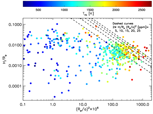
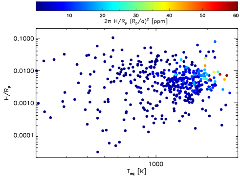
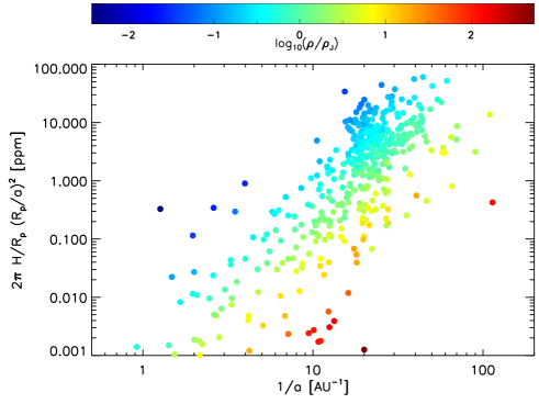
Figure 4: Estimated parameters for the sample of 462 exoplanets considered in the study. In the top graph, the dashed lines divide the parameter space with 2$\pi$$H$/$R_{\rm{p}}$$(R_{\rm{p}}/a)^{2}$ $>$ or $<$ the quoted ppms. From left to right, the dashed lines represent 5, 10, 15, 20 and 25 parts per million. The planet and stellar parameters were extracted from exoplanets.org and complemented from exoplanetarchive.ipac.caltech.edu.

Atmospheric temperature will surely play a key role in the occurrence and optical properties of aerosols. It is thus interesting that the equilibrium temperature of planets with $2\pi(H/R_{\rm{p}})(R_{\rm{p}}/a)^{2}$$>$1 ppm covers a broad range from 410 to 2600 K. The main conclusion of Table (2) and Fig. (4) is that there is a significant number of exoplanets with sufficiently extended atmospheres to potentially exhibit strong forward scattering. Many of these planets have been targets of transit observations.

4 Detectability of forward scattering

To assess how feasible it is the detection of forward scattering, one must also consider the favourable range of phase angles from the observer’s vantage point, in addition to the detailed shape of the planet phase curve and the stellar brightness. To simplify this task, we will assume that: 1) All orbits are circular of radius equal to the orbital semi-major axis; 2) The planet phase curve is binned over two equal-size intervals: [$\alpha_{\rm{A}}$, $\alpha_{\rm{B}}$] and [$\alpha_{\rm{C}}$, $\alpha_{\rm{D}}$], with $\Delta\alpha=\alpha_{\rm{D}}-\alpha_{\rm{C}}=\alpha_{\rm{B}}-\alpha_{\rm{A}}$ (Fig. 1). Forward scattering is strongest over the [$\alpha_{\rm{C}}$, $\alpha_{\rm{D}}$] bin, and we take $\alpha_{\rm{D}}=\alpha_{\rm{I,IV}}\approx\pi-(\rm{R}_{\rm{p}}+R_{\rm{\star}})/a\approx\pi-R_{\rm{\star}}/a$, and $\alpha_{\rm{C}}$=160^∘. The scattering signal is weak over the properly selected [$\alpha_{\rm{A}}$, $\alpha_{\rm{B}}$] control bin, which sets a valid comparison baseline. With these simplifications, we calculated the time elapsed over each interval, $t_{\Delta\alpha}=P\Delta\alpha/2\pi$, where $P$ is the orbital period; 3) The stellar radiation is approximated by a black body at the star effective temperature $T_{\rm{eff}}$ between two wavelengths [$\lambda_{\rm{1}}$, $\lambda_{\rm{2}}$].

Note that the planet does not need to transit in order to produce forward scattering. However, only planets that reach closer to the star than $\alpha$$\sim$160^∘ will produce a measurable effect (see Figs. 1 and 3). Highly inclined orbits will have maximum phase angles $\alpha$$<$$160^{\circ}$ resulting in negligible forward scattering towards the observer. For each planet (and specific $H_{\rm{a}}$, $R_{\rm{p}}$ and $a$; Table 2), we calculated the planet-to-star contrast $F_{\rm{p}}/F_{\star}$ over all phases by interpolating in $H_{\rm{a}}/R_{\rm{p}}$ from our battery of synthetic phase curves. Since the aerosol size is a key parameter that we prescribe but do not predict, we explored the sizes $r_{\rm{eff}}$=0.5, 1 and 2 $\mu$m. We define the observable O as the difference in the average planet-to-star contrast over the forward scattering and control bins: O= $<$$F_{\rm{p}}/F_{\star}$$>$_C→D$-$$<$$F_{\rm{p}}/F_{\star}$$>$_A→B (see Fig. 1).

Photon noise (PN) sets a floor for the detection of the forward scattering signal, and it will be the only term considered in our noise budget. We estimate PN=1/$\sqrt{N_{\Delta\alpha}}$, where $N_{\Delta\alpha}$ is the number of photons collected at the telescope over $t_{\Delta\alpha}$. The expression for PN takes into account two canceling $\sqrt{2}$ and 1/$\sqrt{2}$ factors, one arising from the differential definition of O and one arising from the assumption that the pre- and post-transit observations can be phase-folded to improve PN. We base our calculation of the number of photons at the telescope from an $m_{V}$-magnitude star on the stellar radiated power per unit of area and time. (For completeness, we looked up the visible magnitudes of a few host stars (OGLE-TR-211, WASP-53, -81, -104, WTS-2) on TEPCat (http://www.astro.keele.ac.uk/jkt/tepcat/), and (LUPUS-TR-3) on the Extrasolar Planets Encyclopaedia (exoplanet.eu). For CoRoT-24, we estimated $m_{\rm{V}}$=16 based on a magnitude in R-band of $m_{\rm{R}}$=15.6. For a few Kepler targets (4–8, 10, 15, 43–44, 98, 447), we used their quoted Kepler magnitudes (http://archive.stsci.edu/kepler/kepler$\_$fov/search.php). This ensured that PN could be estimated for all planets with a priori better conditions for forward scattering.) We integrate the Planck function over the specified spectral interval [$\lambda_{1},\lambda_{2}$], and divide by the energy at the given wavelength. Then, using as reference the measured flux of an $m_{V}$=0 star, we estimate the rate:

$$\dot{N}(m_{V})=10^{-0.4m_{V}}f(m_{V}=0;\lambda=550\mbox{ nm})\times$$

$$\int_{\lambda_{1}}^{\lambda_{2}}\frac{\exp{\frac{hc}{(550\mbox{ nm})kT_{\rm{eff}}}}-1}{\exp{\frac{hc}{\lambda kT_{\rm{eff}}}}-1}\left(\frac{550\mbox{ nm}}{\lambda}\right)^{5}\frac{\lambda}{hc}d\lambda$$

Here, $h$ is the Planck constant and $c$ the speed of light. The flux calibration factor $f$($m_{V}$=0; $\lambda$=550 nm)=3.6182$\times$10^-12 W cm^-2 $\mu$m^-1 is taken from Casagrande & VandenBerg (2014). As a check, we confirmed the validity of our estimated photon rates by comparing them to those calculated from star distances and temperatures.

Finally, the number of photons received at the telescope over a time $t_{\Delta\alpha}$ between $\lambda_{1}$=400 nm and $\lambda_{2}$=900 nm is calculated as:

$$N_{\Delta\alpha}=\dot{N}t_{\Delta\alpha}\eta_{\rm{tel}}A_{\rm{tel}}.$$

For the telescope collecting area, we adopt $A_{\rm{tel}}$=$\pi/4$ m², and include an overall instrument efficiency $\eta_{\rm{tel}}$=0.75 that accounts for the CCD quantum efficiency and possible tranmission/reflection losses. This instrument configuration is loosely related to the Kepler telescope (Borucki et al., 2003).

In our feasibility analysis, we also assumed that the composition of the prevailing aerosols is FeO. This condensate absorbs significantly at wavelengths between 0.5 and 2 $\mu$m (Fig. 2). The motivation for this choice is to show that planets that appear dark at small phase angles may result in strong forward scattering. For this optical phenomenon to occur, particle size is more critical than the single scattering albedo. Thus, FeO may be regarded as a proxy for the effect of dark haze particles that might exist in the upper atmosphere of some exoplanets.

Setting $\alpha_{\rm{D}}$$=$$\alpha_{\rm{I,IV}}$, the optimal $\Delta$$\alpha$ depends on the trade-off between the brightness curve shape and associated PN. In the point-like star limit considered in the preparation of Table (2), large aerosols tend to focus most of the scattered starlight on a narrow range of phase angles near $\alpha$=180^∘. In turn, small particle sizes generally result in forward scattering that is less pronounced but spreads over a broader range of phase angles. Implementing a small $\Delta$$\alpha$ enhances the planet-to-star contrast over the forward scattering bin at the cost of reducing the integration time and therefore worsening PN. For simplicity, we adopted $\Delta$$\alpha$=$\alpha_{\rm{I,IV}}$$-$160^∘ (i.e. $\alpha_{\rm{C}}$=160^∘) in all cases, but note that this choice may be sub-optimal and therefore leaves room for improvement of the O/PN ratio. The choice of $\alpha_{\rm{A}}$ and $\alpha_{\rm{B}}$ is such that $<$$F_{\rm{p}}/F_{\star}$$>$_A→B$\approx$0.

Table (2) summarizes the estimated O^0.5μm, O^1μm and O^2μm (each exploring the quoted aerosol particle radius) and PN. A few comments are due. Obviously, the process of averaging over $\Delta$$\alpha$ and having $\alpha_{\rm{D}}$$<$180^∘ dilutes the observable O below the predicted forward scattering peak at $\alpha$=180^∘. Particles that are small result in little forward scattering. Particles that are large result in significant forward scattering, but most of the scattered starlight focuses on phase angles that are unobservable (at least in the point-like star limit) and therefore do not contribute towards O. As a result, the highest Os often occur for the intermediate $r_{\rm{eff}}$$\sim$1 $\mu$m. In a few cases, O$\sim$20–30 ppm values are predicted. We emphasize that, as shown below for the specific case of CoRo-T-24b, considering the finite angular size of the star will tend to increase the predicted Os by factors of up to a few from the values quoted in Tables (2)–(3). The comparison of O and PN shows that photon noise should not be critical for a number of planets provided that multiple orbits can be stacked to improve the O/PN ratio. Some of the planets listed in Table (2) have been observed at out-of-transit phases with precisions comparable to the quoted Os, in particular the Kepler planets (Table 3). It is left for future work the re-analysis of their phase curves in the specific search for forward scattering.

4.1 Low-mass, low-density planets

We next turn our attention to the low-mass, low-density, sub-Neptune CoRoT-24b ($T_{\rm{eq}}$=935 K, $M_{\rm{p}}$/$M_{\rm{J}}$$<$0.018, $\rho_{\rm{p}}$/$\rho_{\rm{J}}$$<$0.5). Recent work (Lammer et al., 2016) has proposed that the measured transit radius probes a low-pressure region high in the atmosphere, and that the opacity is due to an undetermined condensate capable of continuum extinction. The hypothesis of high-altitude aerosols is in line with some of the interpretations for the transmission spectra of e.g. GJ1214b and GJ436b. What makes CoRoT-24b stand out with respect to better characterized sub-Neptunes is its large $H$/$R_{\rm{p}}$$\sim$0.035. CoRoT-24b may be one of a population of planets in similar conditions (Cubillos et al., 2017; Fossati et al., 2017).

The ratio $H$/$R_{\rm{p}}$ (as given by Eq. 5) is the inverse of the parameter $X$ that appears in thermal evaporation theory and represents the squared ratio of the escape velocity and the most probable velocity of the gas Maxwellian distribution (Chamberlain & Hunten, 1987). Small $X$ values represent favourable conditions for escape. In thermal evaporation theory, though, $X$ is evaluated at the exobase and thus well above the optical radius level at which $H$/$R_{\rm{p}}$ is evaluated. The coincidental structure of $H$/$R_{\rm{p}}$ and $X^{-1}$ suggests that puffy planets also offer good conditions for thermal escape.

We have explored the possibilities offered by CoRoT-24b’s large $H$/$R_{\rm{p}}$ for its characterization at large phase angles. We estimate $(R_{\rm{p}}/a)^{2}$=7.6 ppm, 2$\pi$$R_{\rm{p}}$$H_{\rm{a}}$/$a^{2}$=1.7 ppm, and $\alpha_{\rm{I,IV}}$=175.9^∘. At small phase angles, assuming a geometric albedo $A_{\rm{g}}$$\sim$0.3 (Demory, 2014) (which would preclude an envelope dominated by a dark condensate), the planet-to-star contrast is $\sim$2.3 ppm. Correspondingly, at $\alpha$=180^∘ the contrast can be as high as 1.7$\times$$\mbox{<}p_{\rm{a}}\mbox{>}(\Theta=0)\varpi_{0,\rm{a}}$ ppm, thereby exceeding the contrast at small phase angles if micron-size or larger aerosols prevail at the optical radius level (Fig. 11).

We produced synthetic phase curves for CoRoT-24b with $H$/$R_{\rm{p}}$=0.035. To emphasize the possibilities of large versus small phase angles, we adopted a dark condensate (FeO), and tested $r_{\rm{eff}}$ values of 0.5, 1, 2, 3, 5 and 10 $\mu$m. As usual, we adopted $\alpha_{\rm{D}}$$=$$\alpha_{\rm{I,IV}}$ but unlike in the preparation of Table (2) we explored various bin sizes $\Delta$$\alpha$. Again, the control bin was defined at phases for which the planet appears dark and $<$$F_{\rm{p}}/F_{\star}$$>$_A→B$\approx$0. A set of phase curves was calculated in the point-like star limit. We produced another set of phase curves that consider the finite angular size of the host star. The needed modifications to the original radiative transfer algorithm (García Muñoz & Mills, 2015) are described in Appendix C.

Figure (5) shows the two sets of curves with emphasis on the large phase angles. At the top, we show simulations for the various particle sizes in both the point-like star limit (solid) and in the finite angular size star approach (dashed) for the stellar angular radius specific to CoRoT-24b, $\theta_{\star}$$\approx$4.1^∘. To convert from $A_{\rm{g}}$$\Phi(\alpha)$ to planet-to-star contrasts, the scaling factor is 7.6 ppm. For illustration purposes, the Middle and Bottom plots show additional calculations for $\theta_{\star}$$\approx$10 and 20^∘, and $H_{\rm{a}}$/$R_{\rm{p}}$=0.035 as in the initial configuration.

The most obvious effect of considering the finite angular size of the star is that the out-of-transit brightness of the planet ($\alpha$$\lesssim$180^∘$-$$\theta_{\star}$) tends to become larger than in the point-like star limit. This a direct consequence of the convolution of $p_{\rm{a}}$$(\theta$) over the stellar disk brightness to produce $\mbox{<}p_{\rm{a}}\mbox{>}$$(\Theta$). Thus, near transit the planet terminator forward-scatters photons with deflection angles within a $\pm$$\theta_{\star}$ range as for photons coming from the stellar centre. At mid-transit ($\alpha$$\equiv$180^∘) the amount of starlight forward scattered by the atmosphere is lower in the finite angular size limit because the planet sees stellar photons arriving from a range of directions, some of them not overlapping with the peak of the $p_{\rm{a}}$$(\theta$) function (Fig. 11). The attenuating effect of the finite angular size of the star for radiation scattered at $\alpha$$\equiv$180^∘ is more pronounced for the large scattering particles associated with a narrow forward scattering peak $p_{\rm{a}}$$(\theta$=0).

Table (4) summarizes our estimates for the observable O, in both the point-like (regular typeface) and finite angular size (bold typeface) treatments of the star. Their inter-comparison indicates that the point-like star treatment can underestimate the observable by factors of up to a few depending on the combination of $\alpha_{\rm{C}}$, $\theta_{\star}$ and $r_{\rm{eff}}$. For CoRoT-24b, O reaches up to $\sim$10–20 ppm when $\Delta$$\alpha$ is small enough that the steepest part of the brightness surge is resolved. The table also shows the photon noise PN per orbit, which goes from $\sim$64 ppm for $\alpha_{\rm{C}}$=160^∘ to $\sim$186 ppm for $\alpha_{\rm{C}}$=174^∘. Thus, O/PN$<<$1 over the $\Delta$$\alpha$ bin sizes explored. Although signals weaker than $\sim$10 ppm have been detected with Kepler, improving the O/PN ratio to detectable levels calls for one or more of the following strategies: accumulating data from numerous orbits; focusing on planets around bright stars; stacking observations from multiple planets with similar characteristics (e.g. Sheets & Deming, 2014). Ultimately, Table (4) suggests that there is a chance for low-density exoplanets that are too small or dark for detection in occultation to be detected through forward scattering.

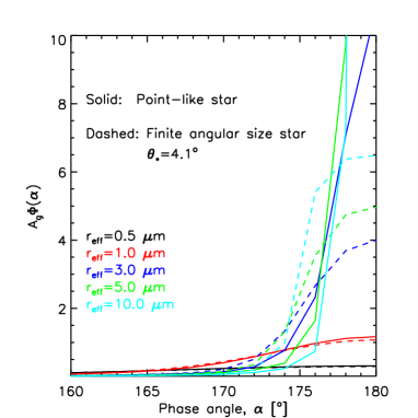
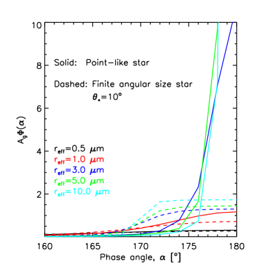
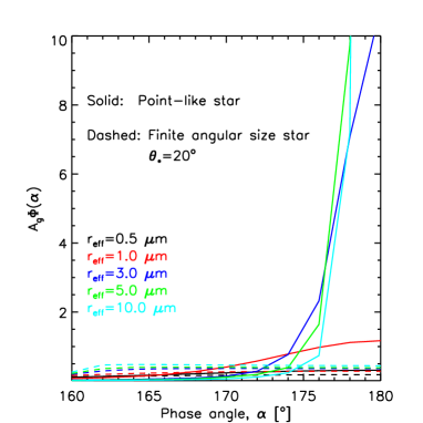
Figure 5: Top. Phase curve simulations of CoRoT-24b ($H_{\rm{a}}$/$R_{\rm{p}}$$\sim$0.035, see text). Taking into account the finite angular size of the star in $<$$p_{\rm{a}}$($\Theta$)$>$ (Fig. (11)) results in the leakage of brightness from the larger to the smaller phase angles. To convert to planet-to-star contrasts, the quoted $A_{\rm{g}}$$\Phi$($\alpha$) should be multiplied by $(R_{\rm{p}}/a)^{2}$=7.6 ppm. Middle and Bottom. Phase curves for $H_{\rm{a}}$/$R_{\rm{p}}$$\sim$0.035, but with the star spanning larger fractions of the sky as viewed from the planet.

Table 4: Forward scattering from CoRoT-24b. We have varied both $\Delta$$\alpha$ (by varying $\alpha_{\rm{C}}$) and $r_{\rm{eff}}$. The tabulated values provide the estimated photon noise PN and the observable O for each aerosol size. The quoted Os in regular typeface refer to calculations in the point-like star limit. Bold typeface refers to calculations taking into account the finite angular size of the star.

$\alpha_{\rm{C}}$	PN	O0.5μm	O1μm	O2μm	O3μm	O5μm	O10μm
[∘]	[ppm]	[ppm]	[ppm]	[ppm]	[ppm]	[ppm]	[ppm]
160.	64.3	1.4	2.7	3.0	2.3	1.5	0.8
		1.4	2.6	3.3	3.5	3.4	3.7
162.	68.8	1.5	3.0	3.4	2.6	1.7	0.9
		1.4	2.9	3.7	3.9	3.9	4.2
164.	74.2	1.6	3.4	3.9	3.0	1.9	1.0
		1.5	3.3	4.3	4.6	4.5	4.9
166.	81.4	1.6	3.8	4.6	3.6	2.3	1.2
		1.6	3.7	5.1	5.4	5.3	5.8
168.	91.1	1.7	4.4	5.5	4.4	2.8	1.4
		1.7	4.2	6.1	6.6	6.5	7.2
170.	105.4	1.8	5.0	6.9	5.6	3.5	1.8
		1.7	4.7	7.5	8.4	8.5	9.5
172.	129.6	1.9	5.7	8.9	7.6	4.7	2.4
		1.8	5.3	9.3	11.2	11.8	13.8
174.	185.6	1.9	6.5	12.2	11.3	7.4	3.5
		1.9	5.9	11.7	15.4	17.7	23.3

4.2 Pre-ingress and post-ingress forward scattering

A number of Kepler planets exhibit brightness peaks that occur at phases somewhat displaced from full illumination (e.g. Demory et al., 2013; Angerhausen et al., 2015; Esteves et al., 2015). For the less strongly irradiated planets, this finding is often explained as caused by clouds forming on the nightside that move onto the dayside and then evaporate, thereby causing an asymmetry in the phase curve (García Muñoz & Isaak, 2015; Shporer & Hu, 2015). If the non-uniform cloud reaches to the altitudes probed by forward scattering, it is conceivable that the pre-ingress and post-ingress brightness curves will have dissimilar slopes.

We can estimate the importance of this with the simplified model sketched in Fig. (6, Top) as applied to a CoRoT-24b-like planet. In this model, one of the terminators (L) is aerosol-free and therefore forward scattering from it is inefficient, whereas the other terminator (R) contains aerosols that scatter efficiently in the forward direction. The aerosols are vertically distributed with a scale height $H_{\rm{a,R}}$/$R_{\rm{p}}$=0.035 and have effective $\mbox{<}p_{\rm{a,R}}\mbox{>}$($\Theta$) as shown in Fig. (11) for various particle sizes and $\theta_{\star}$=4.1^∘.

Figure (6, Bottom) shows the synthetic phase curves. The most remarkable characteristic is that the ingress is brighter than the egress. The reason for this is that at ingress the hazy terminator is seen with a local phase angle that is larger (and the scattering angle smaller) than the aerosol-free terminator. The difference in phase angles between terminators roughly scales as $2R_{\rm{p}}/a$. The magnitude of this angular resolution element and the details of $\mbox{<}p_{\rm{a,R}}\mbox{>}$($\Theta$) dictate the differences in the ingress/egress curves.

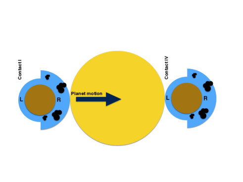
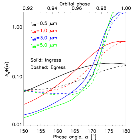
Figure 6: Top. The cartoon depicts a transiting planet at 1st and 4th contacts. The planet’s R terminator scatters the incident starlight in the forward direction much more efficiently than the L terminator. This is potentially due to a more extended aerosol layer and/or larger aerosol particles at the R terminator. Bottom. Phase curves for a CoRoT-24b-like planet with a hazy terminator (R) and an aerosol-free terminator (L). Both ingress and egress curves are shown. Contact I and IV are at $\alpha$$\sim$175.9^∘. The simulations take into account the finite angular size of the star.

5 Blending with other photometric effects

5.1 Modulations from stellar tides

The measured brightness from a close-in planet-star system includes the contribution from the planet atmosphere together with modulations due to Doppler beaming and tidal ellipsoidal distortion of the star. The magnitude, period and lag with respect to the orbital motion of these modulations are sources of information on both the planet and the star (e.g. Shporer, 2017, for a recent review).

Assuming that the planet is on a circular orbit and the planet-star system is seen edge-on, the brightness modulation from Doppler beaming is $\propto$sin($\alpha$), whereas the modulation due to ellipsoidal distortion is $\propto$cos($2\alpha$) with additional correcting terms $\propto$cos($\alpha$) and cos(3$\alpha$). The theoretical treatment of these phenomena provides expressions for the coefficients of each term, which depend on e.g. $a$, $R_{\star}$, $M_{\rm{p}}$ and $M_{\star}$ (Morris & Naftilan, 1993; Loeb & Gaudi, 2003). The planet atmosphere modulates the planet-star system brightness in two different ways. Thermal radiation prevails when the atmosphere is hot and/or the observations are made at long wavelengths. Reflected starlight dominates at low temperatures and/or short wavelengths. With enough photometric precision and multi-wavelength observations, it is possible to disentangle these phenomena, also the two atmospheric terms (Placek et al., 2016), by fitting the observations to models (e.g. Angerhausen et al., 2015; Esteves et al., 2015).

The photometric effects described above may blend in the observed brightness signal and cause degeneracies in the interpretation of the inferred physical properties (Mislis & Hodgkin, 2012). Aggravated by moderate signal-to-noise ratios and a possibly incomplete understanding of each photometric effect, these difficulties may be at the heart of the mass discrepancy reported for some planet-star systems (Shporer, 2017). Indeed, it has become apparent that the planet masses inferred from photometric measurements (through Doppler beaming or tidal ellipsoidal distortions) and from radial velocities are at times mutually inconsistent.

Figure (7) suggests that forward scattering from a horizontally uniform planet will leak into cos($2\alpha$) and higher order even cosine harmonics, thereby blending with the stellar tide modulation. The overall effect is a partial cancellation of the ellipsoidal effect, particularly at large phase angles and if the angular size of the star is also large, and in turn a reduced planetary mass as estimated from this photometric effect. We have briefly explored to what extent forward scattering affects the photometric mass inferred from the stellar tide modulations in the cases of TrES-2b (Barclay et al., 2012) and Kepler-76 b (Faigler et al., 2013), with quoted ellipsoidal semi-amplitudes of 2.8 and 21.5 ppm, respectively. We find that 2$\pi$$R_{\rm{p}}$$H_{\rm{a}}$/$a^{2}$$\sim$5 (TrES-2b) and $\sim$10 (Kepler-76b) ppm, which means that blending of forward-scattered starlight with the tidal brightness modulation is a priori possible. The fact that the masses retrieved from stellar tide modulations ($M^{\rm{ell}}_{\rm{p}}$/$M_{\rm{J}}$=1.06${}^{+0.28}_{-0.23}$ for TrES-2b, and 2.1$\pm$0.4 for Kepler-76b) and radial velocities for both planets ($M^{\rm{RV}}_{\rm{p}}$/$M_{\rm{J}}$=1.206$\pm 0.045$ for TrES-2b, and 2.00$\pm$0.26 for Kepler-76b) are in good agreement (Barclay et al., 2012; Faigler et al., 2013) suggests that neither of these planets exhibit significant forward scattering, which puts an additional constraint on their atmospheres.

It is worth noting the cases of Kepler-12b and -412b, listed on Tables (2)–(3), whose phase curves have been published by Angerhausen et al. (2015) and Esteves et al. (2015). Kepler-12b’s curve is distinctly asymmetric with respect to occultation, a fact likely attributable to a horizontally non-homogeneous atmosphere. Other Kepler planets also show asymmetric atmospheric contributions (Angerhausen et al., 2015; Esteves et al., 2015). According to our estimates, both planets might exhibit forward scattering signals of up to 10-20 ppm. A look at the corresponding curves in Esteves et al. (2015) however does not reveal clear evidence for forward scattering in the case of Kepler-412b, although it hints at a tentative brightness surge at orbital phases close to one in the case of Kepler-12b. A thorough analysis incorporating the data from all Kepler quarters might provide a more definitive answer.

Clearly, further work is needed to quantify these contributions and extend the analysis to all planets with accurate photometric data available. Because the forward scattering signal scales as $M^{-1}_{\rm{p}}$ and $a^{-5/2}$ (Eq. 7), and the amplitude of the ellipsoidal tidal distortion scales as $M_{\rm{p}}$ and $a^{-3}$, each effect will likely dominate in a different region of the $M_{\rm{p}}$–$a$ parameter space.

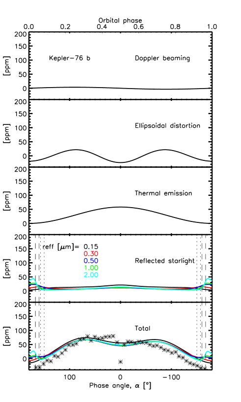
Figure 7: Photometric modulations for a Kepler-76b-like planet. The Doppler beaming and ellipsoidal distortion contributions are based on Esteves et al. (2015). We model the thermal emission component as (1+cos($\alpha$))/2, premultiplied by a coefficient of 58 ppm consistent with integrated blackbody radiation between 0.45 and 0.85 $\mu$m for an estimated $T_{\rm{eq}}$=2551 K. The reflected starlight calculations are based on a FeO aerosol, which explains the low reflectance at small phase angles. As in the case of CoRoT-24 b (Figs. 5-6), the multiple scattering simulations were done considering the finite size of the star, and $\theta_{\star}$$\approx$12.8^∘. The symbols in the bottom plot are the measurements reported by Esteves et al. (2015) in their Fig. 3, shifted in the vertical by 30 ppm. The vertical lines in the two bottom graphs represent the positions for [$\alpha_{\rm{A}}$, $\alpha_{\rm{B}}$] (dotted) and [$\alpha_{\rm{C}}$, $\alpha_{\rm{D}}$] (dashed) as described in the preparation of Table (2).

5.2 Transits

During a transit, the host star dims by an amount that depends on the planet size and its atmospheric structure. For an exponential atmosphere described by a single absorber (the conditions explored here), and omitting the scattering towards the observer of photons having one or more collisions in the atmosphere, the planet appears effectively opaque up to the so-called equivalent height $h_{\rm{eq}}(\lambda)$. To a good approximation, the equivalent height occurs where the limb opacity of the atmosphere $\tau_{\rm{limb}}$=0.56 (Karkoschka et al., 1997; Lecavelier des Etangs et al., 2008).

Part of the starlight that is intercepted by the atmosphere during the transit is restored into the forward direction and scattered towards the observer (Brown, 2001; Hubbard et al., 2001; García Muñoz et al., 2012; García Muñoz & Mills, 2012; De Kok & Stam, 2012; Robinson, 2017). Under the assumption of an exponential atmosphere, Eq. (21) quantifies how many of these photons reach the observer, thereby reducing the transit depth by 2$R_{\rm{p}}$$\Delta$/$R_{\star}^{2}$ or the equivalent to an annulus area of radius $R_{\rm{p}}$ and width $\Delta$:

$$\frac{\Delta}{H_{\rm{a}}}=\pi\left(\frac{R_{\star}}{a}\right)^{2}\mbox{<}p_{\rm{a}}\mbox{>}(\Theta=0)\varpi_{0,\rm{a}}.$$ (8)

This is also akin to diminishing the transmission-only equivalent height, $h_{\rm{eq}}$, by $\Delta$, which means that the measurable equivalent height during the transit is $h^{\prime}_{\rm{eq}}$=$h_{\rm{eq}}$$-$$\Delta$ rather than $h_{\rm{eq}}$. $\Delta$ depends on wavelength through the aerosol properties $\mbox{<}p_{\rm{a}}\mbox{>}$$(\Theta$$=$$0)$ and $\varpi_{0,\rm{a}}$. Typically, the larger the particle radius $r_{\rm{eff}}$ the larger the effective $\mbox{<}p_{\rm{a}}\mbox{>}$($\Theta$=0) (Fig. 11), and in turn the impact of forward scattering on the transit depth. In an aerosol-rich atmosphere, $\varpi_{0,\rm{a}}$ will depend strongly on wavelength if there are strong gas absorption bands in the spectral range of interest. Within the gas absorption band, $\varpi_{0,\rm{a}}$ can become significantly smaller than in the continuum, and in turn $h^{\prime}_{\rm{eq}}$$\approx$$h_{\rm{eq}}$ at the specific wavelengths.

Interestingly, the angular size of the star enters into Eq. (8) both directly ($\theta_{\star}$$\approx$$R_{\star}$/$a$) and indirectly through $\mbox{<}p_{\rm{a}}\mbox{>}$($\Theta$=0) (Eq. 13, Fig. 11). The two effects partially cancel out. For large orbital distances, the $a^{2}$ term in the denominator of Eq. (8) dominates and $\Delta$/$H_{\rm{a}}$ becomes small; for small orbital distances, the convolution of $p_{\rm{a}}$($\theta$) over an extended solid angle results in a reduced $\mbox{<}p_{\rm{a}}\mbox{>}$($\Theta$=0) with respect to $p_{\rm{a}}$($\theta$=0). Figure (9) incorporates the information presented in Fig. (11) for $\mbox{<}p_{\rm{a}}\mbox{>}$($\Theta$=0) and shows that forward scattering will reduce the equivalent height of the atmosphere by typically less than one scale height, even for the more extreme configurations ($\theta_{\star}$=20^∘, $r_{\rm{eff}}$=10 $\mu$m). The connection of $\Delta$ with the particle size is more direct through the analytical expression of Eq. (8) than in the treatments by De Kok & Stam (2012) and Robinson (2017), who base their analyses on Henyey-Greenstein parameterizations of the aerosols scattering phase function.

For completeness, Fig. (8) shows the transit depth as a function of orbital phase for both CoRoT-24 b and Kepler-76 b. For CoRoT-24 b ($\theta_{\star}$$\approx$4.1^∘), it is shown the case with aerosols of particle size $r_{\rm{eff}}$=10 $\mu$m, which results in a correction of the transit depth at mid-transit due to forward scattering of about 50 ppm. For Kepler-76 b ($\theta_{\star}$$\approx$12.8^∘), the corresponding graph shows the case with $r_{\rm{eff}}$=2 $\mu$m, which results in a correction of about 36 ppm. Both corrections correspond to a change in the equivalent height of less than their estimated gas pressure scale heights.

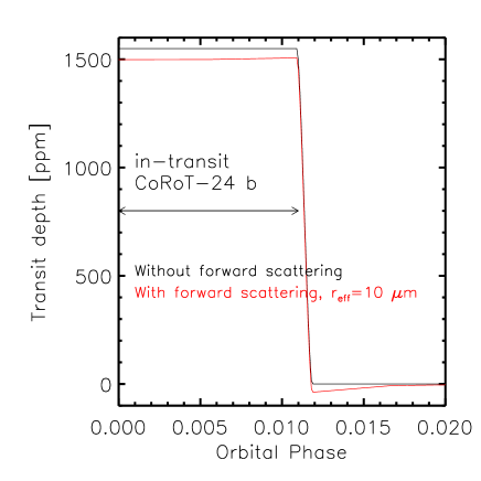
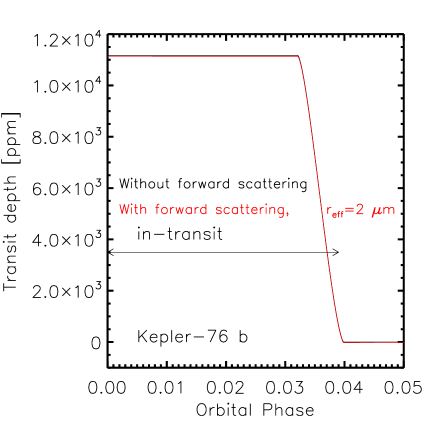
Figure 8: Transit depth as a function of orbital phase. For the transit light curve, we assumed the brightness is uniform over the stellar disk. Forward scattering reduces to some extent the transit depth. In the two examples shown here, the reduction amounts to $\sim$50 ppm (CoRoT-24 b) and $\sim$36 ppm (Kepler-76 b), which is less than the equivalent to a gas pressure scale height.

We have assumed throughout this work an effective wavelength $\lambda_{\rm{eff}}$=0.65 $\mu$m. Because in Mie theory the diffraction peak of the aerosols is largely dictated by the size parameter $x_{\rm{eff}}$=2$\pi$$r_{\rm{eff}}$/$\lambda_{\rm{eff}}$, Fig. (9) can be reworked at other wavelengths by appropriately selecting the particle radius.

DeVore et al. (2016) have shown that forward scattering can significantly modify the transit light curve of ultra-short period planets surrounded by dust clouds. The difference with our treatment is that these authors assume that the entire (and sizable) cloud is uniform in its dust content, and thus every element of it can scatter the incident starlight towards the observer. In our treatment, the exponential variation of the optical properties reduces the effective scattering area to a relatively narrow ring around the planet of width about an atmospheric scale height.

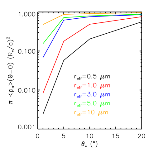
Figure 9: Forward scattering contribution to the equivalent height of the atmosphere, normalized by the scale height and adopting $\varpi_{\rm{0,a}}$=1, according to Eq. (8). Each curve assumes aerosols of a specific particle radius. The values of $\mbox{<}p_{\rm{a}}\mbox{>}$($\Theta$=0) are from Fig. (11). According to these curves, forward scattering will reduce the measured equivalent height of the atmosphere by less than one scale height, even in the most extreme conditions of particle size and star angular radius explored here.

6 Summary

A main goal of this work is to raise awareness about the diagnostics possibilities of exoplanet brightness measurements at large phase angles. As for Saturn’s moon Titan, a brightness surge when the planet approaches back-illumination will provide joint information on atmospheric stratification and aerosol optical properties. This is valuable insight difficult to gain by other means. It is unclear how common this optical phenomenon is, but its possibility justifies a dedicated search with existing and future observations.

In the framework of exponential atmospheres, we derived an analytical expression for forward-scattered starlight in the single-scattering limit. The expression incorporates the effects of the angular size of the star, one of which is to convolve the aerosols scattering phase function with the brightness distribution over the stellar disk. Based on this expression, we estimate that there are a number of exoplanets with a priori suitable conditions for forward scattering. We have refined these predictions with a more elaborate assessment that considers the shape of the phase curve and the time elapsed during the brightening phase. Some of these planets potentially exhibit brightness surges of up to tens of ppms.

At out-of-transit phases, considering the finite angular size of the star tends to increase the amount of starlight forward-scattered towards the observer with respect to the treatment in the point-like star limit. On the contrary, during the transit the finite angular size of the star reduces the amount of starlight that reaches the observer with respect to the point-like star limit. Once the latter effect is considered, it is seen that forward scattering will modify the equivalent height of the atmosphere by less than one scale height in most configurations. For future reference, we show how to take into account the finite angular size of the star in Backward Monte Carlo radiative transfer models. Our study raises the possibility that, given the appropriate atmospheric structure, some low-density planets may be easier to detect at large phase angles than in occultation.

Throughout our treatment, we assumed that aerosols dominate the atmospheric opacity at the optical radius level. Two additional key assumptions are that the aerosols are vertically distributed with a scale height equal to the gas scale height, and that the aerosols are described as having a single particle size that we prescribe but do not predict. This simplified treatment is similar to the way transit spectra are often interpreted within retrieval algorithms. The reality of exoplanet atmospheres will surely be more complex, but our simplified approach at least enables a direct comparison with observations from which to draw physical conclusions. It may well happen that some of the planets that are ranked higher as candidates for strong forward scattering will have no detectable signal because their atmospheres do not form aerosols or the aerosol particles at the optical radius level are not large enough. Even then, and if observations of high enough precision exist, a non-detection will provide constraints on the atmospheric structure that can be tested against microphysical models. This possibility should motivate further studies on the microphysics of aerosols in the diverse range of conditions found in exoplanet atmospheres (e.g. Helling & Fomins, 2013; Lavvas et al., 2013; Lavvas & Koskinen, 2017; Lee et al., 2016). Helpful information that could be obtained from such investigations includes: the aerosol scale height at the optical radius level, and the particle size of the condensates dominating the continuum opacity at the corresponding altitudes.

Last, we emphasize that the starlight reflected by exoplanets varies with phase in manners that are not necessarily well described by simple formulations such as Lambert’s law. It is challenging to decide when more elaborate descriptions are justified, but it is equally important to realize that oversimplified descriptions will likely wash out unique information on the planet atmosphere.

Appendix A Starlight forward-scattered by a planet. An analytical expression for exponential atmospheres.

We derive an expression for the starlight forward-scattered by an exponential atmosphere at a phase angle of 180^∘. In its general form, the expression considers the finite angular size of the star. A few simplifying assumptions (SAs) enable us to treat the problem analytically:

1. The atmosphere is horizontally uniform but vertically stratified.

2. The optical properties of the atmosphere are determined by ubiquitous particles that are referred to as aerosols (subscript _a) but that may actually be a mix of gases and condensates.

3. The aerosols extinction and scattering coefficients, $\gamma_{\rm{a}}$ and $\beta_{\rm{a}}$, drop exponentially in the vertical with the scale height $H_{\rm{a}}$. The single scattering albedo $\varpi_{\rm{0,a}}$$=$$\beta_{\rm{a}}$/$\gamma_{\rm{a}}$ is altitude-independent.

4. The aerosols scattering phase function $p_{\rm{a}}(\theta)$ is also altitude-independent. $\theta$ is the scattering angle between the incident and exit directions of a photon being scattered by an aerosol particle.

5. The ratio of the aerosol scale height $H_{\rm{a}}$ and the planet radius $R_{\rm{p}}$ satisfies $H_{\rm{a}}/R_{\rm{p}}$$<<$1.

6. The starlight forward-scattered by the atmosphere is dominated by singly-scattered photons. The validity of this assumption is tested a posteriori in Appendix B by comparison with numerical solutions to the multiple-scattering problem.

Figure (10) sketches the star-planet-observer configuration at mid-transit for an impact parameter equal to zero, when $\alpha$ is identically equal to 180^∘. The radiance at $\mathbf{x}$ in direction $\mathbf{s}$ due to stellar photons that either go through the atmosphere without scattering (and without altering their trajectories by atmospheric refraction) or that are scattered once is:

$$I\mathbf{(x,s)}=t(\mathbf{x,x_{\rm{b}}})I\mathbf{(x_{\rm{b}},s)}+\int_{\mathbf{x_{\rm{b}}}}^{\mathbf{x}}d\ell{{}_{\rm{a}}}t(\mathbf{x,x_{\rm{a}}})\beta(\mathbf{x_{\rm{a}}})\times$$ (9)

$$\times\int_{\Omega_{\star}}d\Omega(\mathbf{s^{\prime}}){p_{\rm{a}}(\mathbf{x_{\rm{a}},\mathbf{s^{\prime}}})}I\mathbf{(x_{\rm{a}},\mathbf{s_{\star}})}.$$

Here, $t(\mathbf{x,x_{\rm{a}}})$ and $t(\mathbf{x,x_{\rm{b}}})$ are the atmospheric transmittances between $\mathbf{x}$ and $\mathbf{x_{\rm{a}}}$, and between $\mathbf{x}$ and $\mathbf{x_{\rm{b}}}$, respectively. $I\mathbf{(x_{\rm{b}},s)}$ is the outgoing radiance in direction $\mathbf{s}$ from the stellar surface element at $\mathbf{x_{\rm{b}}}$. For simplicity, we assume that the star emits as a blackbody of radiance $B_{\star}$, and omit limb darkening, which means that $I\mathbf{(x_{\rm{b}},s)}$$=$$B_{\star}$. $d\ell{{}_{\rm{a}}}$ is the differential arc-length along $\mathbf{s}$ at $\mathbf{x_{\rm{a}}}$, and $\beta(\mathbf{x_{a}})$ is the scattering coefficient of the medium at $\mathbf{x_{\rm{a}}}$. The second integral represents the starlight that is scattered at $\mathbf{x_{\rm{a}}}$ into direction $\mathbf{s}$ from all directions $\mathbf{s_{\rm{\star}}}$ emerging at the stellar surface. The scattering angle $\theta$ is locally defined by the dot product of the $\mathbf{s}$ and $\mathbf{s}_{\star}$ directions, $\cos{\theta}$$=$$\mathbf{s}\cdot\mathbf{s}_{\star}$, and is equal to zero in forward scattering. $d$$\Omega$ is the differential solid angle subtended by the star from $\mathbf{x_{\rm{a}}}$, and ${p_{\rm{a}}(\mathbf{x_{\rm{a}},\mathbf{s^{\prime}}})}$ is the corresponding aerosol scattering phase function. We normalize ${p_{\rm{a}}(\theta)}$ (SA4) so that its integral over the 4$\pi$ solid angle is one. This normalization differs from the more conventional approach of making the integral of ${p_{\rm{a}}(\theta)}$ over all directions equal to 4$\pi$. In our normalization, for isotropic scattering ${p_{\rm{a}}(\theta)}$=1/4$\pi$, and for Rayleigh scattering ${p_{\rm{a}}(\theta)}$=1/4$\pi$ (1$+$$\cos^{2}{\theta}$).

For evaluating the second integral of Eq. (9), we adopt $I\mathbf{(x_{\rm{a}},\mathbf{s_{\star}})}$$\approx$$B_{\star}$$t(\mathbf{x_{\rm{a}},x_{\rm{b}}})$, which assumes that the opacity from $\mathbf{x_{\rm{a}}}$ to $\mathbf{x_{\rm{b}}}$ is representative of the opacity from $\mathbf{x_{\rm{a}}}$ in any of the possible $-\mathbf{s_{\rm{\star}}}$ directions towards the star. Also, we take $d$$\Omega$$\approx$2$\pi$$d$($\cos{\theta}$), which tacitly assumes that all points $\mathbf{x_{\rm{a}}}$ are near the planet-star axis. With this, the integral becomes:

$$2\pi B_{\star}t(\mathbf{x_{\rm{a}},x_{\rm{b}}})\int_{\cos{\theta_{\star}}}^{1}d(\cos{\theta})p_{\rm{a}}(\theta),$$ (10)

where $\cos\theta_{\star}$=$\sqrt{1-(R_{\star}/a)^{2}}$. As usual, $R_{\star}$ and $a$ are the stellar radius and planet orbital distance, respectively. The integral of Eq. (10) has the meaning of an aerosol scattering phase function averaged over the angular size of the star and, in general, requires numerical evaluation. We term this general treatment the finite angular size star approach, and is relevant when the angle $\theta_{\star}$ subtended by the star from the planet is not small. In contrast, the so-called point-like star approach is appropriate when the planet-star orbital distance is large enough that all stellar photons reaching the planet can be assumed to be collimated and $\theta_{\star}$$\rightarrow$0. In this latter approach, Eq. (10) can be simplified further into:

$$\pi\left(\frac{R_{\star}}{a}\right)^{2}B_{\star}t(\mathbf{x_{\rm{a}},x_{\rm{b}}})p_{\rm{a}}(\theta=0).$$ (11)

For convenience, we introduce an aerosol scattering phase function averaged over the stellar angular size:

$$\mbox{<}p_{\rm{a}}\mbox{>}(\Theta=0)=2\left(\frac{a}{R_{\star}}\right)^{2}\int_{\cos{\theta_{\star}}}^{1}d(\cos{\theta})p_{\rm{a}}(\theta),$$ (12)

and rewrite Eq. (10) as:

$$\pi\left(\frac{R_{\star}}{a}\right)^{2}B_{\star}t(\mathbf{x_{\rm{a}},x_{\rm{b}}})\mbox{<}p_{\rm{a}}\mbox{>}(\Theta=0)$$ (13)

which encompasses both Eqs. (10) and (11). Obviously, in the point-like star limit, $\mbox{<}p_{\rm{a}}\mbox{>}(\Theta=0)$$\rightarrow$$p_{\rm{a}}(\theta=0)$, and Eq. (13) reduces to Eq. (11). Both Budaj et al. (2015) and DeVore et al. (2016) present formulations to calculate $\mbox{<}p_{\rm{a}}\mbox{>}(\Theta)$ for conditions other than $\Theta$=0, using either Mie theory or Airy functions in the description of the scattering phenomenon. Using $\mbox{<}p_{\rm{a}}\mbox{>}(\Theta)$ rather than $p_{\rm{a}}(\theta)$ in the radiative transfer problem when evaluating the contribution from the star at each photon-atmospheric particle scattering collision (through integrals like the second one in Eq. (9)) reduces the radiative transfer problem with a finite angular size star to the simpler problem of a point-like star.

Figure (11) demonstrates $p_{\rm{a}}(\theta)$ and $\mbox{<}p_{\rm{a}}\mbox{>}(\Theta)$ for FeO particles of a few effective radii $r_{\rm{eff}}$ at an effective wavelength $\lambda_{\rm{eff}}$=0.65 $\mu$m. For $\mbox{<}p_{\rm{a}}\mbox{>}(\Theta)$, we adopted star angular radii $\theta_{\star}$ of 1, 5, 10, and 20^∘. The comparison of our Fig. (11) to Fig. 3 of Budaj et al. (2015) (dividing their results by 4$\pi$) and Fig. 3 of DeVore et al. (2016) shows that all three treatments seem equivalent.

For a spherically symmetric atmosphere, the transmittance $t(\mathbf{x,x_{\rm{b}}})$ ($=$$t(\mathbf{x,x_{\rm{a}}})t(\mathbf{x_{\rm{a}},x_{\rm{b}}})$) can be reduced to a function of the the minimum distance $r$ from the line of sight to the planet centre (SA1). If $\tau(r)$ is the optical thickness along that chord, $t(\mathbf{x,x_{\rm{b}}})$$=$$\exp{(-\tau(r))}$. And from the definition of optical thickness:

$$\tau=\int_{\mathbf{x_{\rm{b}}}}^{\mathbf{x}}d\ell{{}_{\rm{a}}}\gamma(\mathbf{x_{a}}).$$

Following the above, Eq. (9) can be rewritten as:

$$I(r)=B_{\star}\exp{(-\tau(r))}+B_{\star}\pi\left(\frac{R_{\star}}{a}\right)^{2}\varpi_{\rm{0,a}}\tau(r)\exp{(-\tau(r))}\mbox{<}p_{\rm{a}}\mbox{>}(\Theta=0).$$ (14)

Deep into the atmosphere, $\tau(r)$ is large whereas $\exp{(-\tau(r))}$ is small. The reverse is true high up in the atmosphere.

The irradiance measured by the observer from a star-to-Earth distance $d$ is obtained by integration of $I(r)$ over the solid angle subtended by the whole planet-star system:

$$F=\int{Id\Omega}=2\pi\int I(r)\frac{rdr}{d^{2}}.$$ (15)

According to Eq. (14), $F$ contains the contributions from both unscattered photons and from photons that have undergone one scattering collision.

For the unscattered component:

$$F_{0}=\frac{2\pi B_{\star}}{d^{2}}\int_{R_{\rm{0}}}^{R_{\star}}\exp{(-\tau(r))}rdr,$$ (16)

where $R_{\rm{0}}$ is a somewhat arbitrary altitude level in the atmosphere such that $\tau(R_{\rm{0}})$$>>$1. Or, if we introduce the planet equivalent cross section to transmission, $\pi r_{\rm{eq}}^{2}$:

$$F_{0}=\frac{\pi B_{\star}}{d^{2}}\left(R_{\star}^{2}-r_{\rm{eq}}^{2}\right)$$ (17)

For exponential atmospheres, Lecavelier des Etangs et al. (2008) have shown that $r_{\rm{eq}}$ (=$R_{0}$+$h_{\rm{eq}}$) matches the atmospheric level where $\tau(h_{\rm{eq}})$=0.56 that defines the optical radius of a planet, $R_{\rm{p}}$.

Correspondingly, for the single-scattering component:

$$F_{1}=B_{\star}\pi\left(\frac{R_{\star}}{a}\right)^{2}\varpi_{\rm{0,a}}\mbox{<}p_{\rm{a}}\mbox{>}(\Theta=0)\frac{2\pi}{d^{2}}\int_{R_{\rm{0}}}^{R_{\star}}\tau(r)\exp{(-\tau(r))}rdr.$$ (18)

The occurrence of $\tau(r)\exp{(-\tau(r))}$ suggests that the main contribution to the integral arises from $\tau(r)$$\sim$1. From SA1 and SA3, $\tau(r)=\tau(R_{\rm{0}})\exp{(-(r-R_{\rm{0}})/H_{\rm{a}})}$. By virtue of SA5, the integral of Eq. (18) converges rapidly in $r$, and it is acceptable to take $r$$\approx$$R_{\rm{p}}$ outside of the integration (Fig. 12). The resulting integral is easy to evaluate after realizing that $H_{\rm{a}}d\tau=-\tau dr$, and results in:

$$\int_{R_{\rm{0}}}^{R_{\star}}\tau(r)\exp{(-\tau(r))}dr=H_{\rm{a}}(1-\exp(-\tau(R_{\rm{0}})))\approx H_{\rm{a}}.$$ (19)

Introducing these results into $F_{1}$ and normalizing by the irradiance of the unimpeded star at the observer’s vantage point:

$$F_{\star}=B_{\star}\pi\left(\frac{R_{\star}}{d}\right)^{2},$$ (20)

leads to:

$$\frac{F_{1}}{F_{\star}}\approx 2\pi\mbox{<}p_{\rm{a}}(\Theta=0)\mbox{>}\varpi_{\rm{0,a}}\frac{H_{\rm{a}}}{R_{\rm{p}}}\left(\frac{R_{\rm{p}}}{a}\right)^{2},$$ (21)

which is the analytical expression for starlight forward-scattered towards the observer by an exponential atmosphere under the assumption of single scattering, relative to the net stellar brightness.

The orbital distance enters Eq. (21) in two competing ways. Since the amount of starlight intercepted by the planet varies as $a^{-2}$, close-in planets will in principle appear brighter in reflected starlight. However, as the ratio $R_{\star}/a$ becomes larger $\mbox{<}p_{\rm{a}}\mbox{>}$($\Theta$=0) samples scattering angles that differ from the strict forward scattering configuration, and $\mbox{<}p_{\rm{a}}\mbox{>}$($\Theta$=0) will typically become much smaller than $p_{\rm{a}}$($\theta$=0). The decrease in $\mbox{<}p_{\rm{a}}\mbox{>}$($\Theta$=0) with respect to $p_{\rm{a}}$($\theta$=0) is more pronounced when $R_{\star}/a$ (or $\theta_{\star}$) is large and/or the aerosols exhibit a strong forward scattering peak.

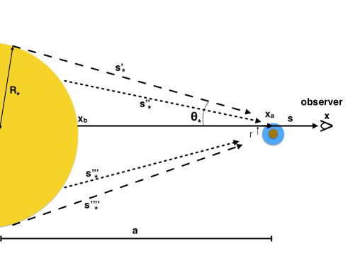
Figure 10: Mid-transit geometry relevant to the derivation of Eq. (21). The various $\mathbf{s_{\star}}$ directions describe radiation rays emerging from the star; their corresponding photons undergo collisions with the atmospheric aerosols at $\mathbf{x_{\rm{a}}}$ and are scattered into direction $\mathbf{s}$ towards the observer. $\theta_{\star}$ is the angular radius of the star from the planet.

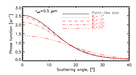
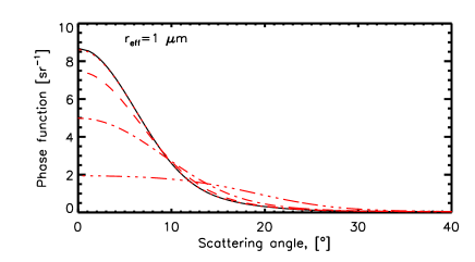
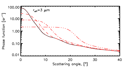
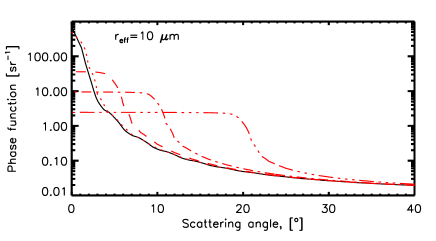
Figure 11: Aerosols scattering phase function in the point-like star limit, $p_{\rm{a}}$($\theta$) (black); and in the finite angular size star approach, $\mbox{<}p_{\rm{a}}\mbox{>}(\Theta)$ (red). Each graph considers aerosols of a specific particle size anf FeO composition. Note the different vertical scales for each of the graphs. The various red curves correspond to different star angular radii. $p_{\rm{a}}$($\theta$) is calculated from Mie theory. For $\mbox{<}p_{\rm{a}}\mbox{>}(\Theta)$, we convolve $p_{\rm{a}}$($\theta$) with the scattering angle for stellar rays from each visible element of the stellar disk. Accounting for the finite angular size of the star decreases the effective scattering by the aerosols at small scattering angles (typically, angles $<$$\theta_{\star}$) but increases it at scattering angles somewhat larger. For sufficiently large scattering angles, both $p_{\rm{a}}$($\theta$) and $\mbox{<}p_{\rm{a}}\mbox{>}(\Theta)$ merge.

Figure 12: Most of the contribution to the starlight forward-scattered by an exponential atmosphere arises from within a few scale heights above and below the optical radius level, defined by the limb opacity $\tau(r=R_{\rm{p}})$=0.56. In the example, $\tau(r)=10\exp(-(r-R_{\rm{0}})/H_{\rm{a}})$. Because, $H_{\rm{a}}/R_{\rm{p}}$$<<$1, the curves for $r\tau(r)\exp{(-\tau(r))}$ and $\tau(r)\exp{(-\tau(r))}$ are nearly undistinguishable in the scale of the plot; only the latter is graphed.

Appendix B Multiple scattering for close-in planets. The $\alpha$=180^∘ configuration.

García Muñoz et al. (2017) show that the number of collisions contributing to Titan’s brightness decreases as the star-object-observer phase angles increases (their Fig. 3). We confirm that for the phase curves presented in our Fig. (3) the difference between the numerical multiple scattering solution at $\alpha$=180^∘ and the single-scattering estimate based on Eq. (21) remained below 30%. Also, for the phase curves in Fig. (5) motivated by the study of CoRoT-24b, in both the point-like and finite angular size treatments of the star, single scattering contributed $\sim$70$\%$ or more to the multiple scattering solution. Using the case of CoRoT-24b, we ran a few additional simulations in which we forced the aerosols to be fully conservative, i.e. $\varpi_{0,\rm{a}}$=1. In those cases, single scattering contributed at least $\sim$50$\%$ of the multiple scattering solution at $\alpha$=180^∘. Together, these conclusions suggest that Eq. (21) generally approximates the planet-to-star contrast in forward scattering to within a factor of two or better.

Appendix C Backward Monte Carlo calculations with a finite angular size star

The radiative transfer calculations presented in this work were done with a Backward Monte Carlo algorithm that has been described elsewhere (García Muñoz & Mills, 2015), and used to investigate the phase curves of exoplanets, Venus and Titan (García Muñoz & Isaak, 2015; García Muñoz et al., 2014, 2017). These previous studies omitted the consideration of the finite angular size of the star, which can modify the effective scattering geometry at the particle level. The effect is likely important for close-in planets at large phase angles because atmospheric aerosols can be efficient at scattering in the forward direction. Referring to Figs. (10) and (13), a scattering particle sees the incident starlight enter the atmosphere from a range of directions s_⋆ rather than from a single direction. This distinction is important since the probability that the incident photon is re-scattered into another direction can be a strong function of the relative angle between the two directions. For instance, in the configuration of Fig. (10), which assumes a perfect star-planet-observer alignment, the angle between s_⋆ and s ranges from 0 to $\theta_{\star}$ (the angular size of the star as viewed from the planet). For very close-in exoplanets, $\theta_{\star}$ can be as large as 20^∘.

Our Backward Monte Carlo algorithm builds the solution to the radiative transfer problem by tracking simulated photons (or photon packages) from the observer’s vantage point through the atmosphere. At the outset of the simulation, each photon is assigned a ‘weight’ of one. As the simulation proceeds and the photon interacts with the medium, its weight is progressively reduced by amounts that account for the probabilities that the photon is either absorbed within or escapes from the atmosphere. The simulated photon trajectory is terminated when the weight falls below a user-defined threshold. A tentative photon trajectory is sketched in Fig. (13). The arrows show the directions for the photon displacements, which are the reverse of the directions actually simulated in the Backward algorithm. At each photon scattering collision, either within the atmosphere or at the planet surface, the algorithm evaluates an integral over solid angle that results into two separate contributions. Mathematically, these contributions are expressed as the two terms on the right hand sides of Eqs. (9)-(10) in García Muñoz & Mills (2015).

The first contribution accounts for diffuse radiation, i.e. radiation associated with photons that have had at least one previous collision. The relevant scattering phase function to quantify the diffuse radiation re-scattered into the $\mathbf{s^{\prime\prime}}$ direction is the local $p_{\rm{a}}$($\theta$) because the change in photon directions from $\mathbf{s^{\prime}}$ to $\mathbf{s^{\prime\prime}}$ is independent of the star location. The corresponding implementation in the algorithm is as described in García Muñoz & Mills (2015). The second contribution accounts for stellar photons having their first scattering collision. Mathematically (Eqs. (9)-(10) in García Muñoz & Mills (2015), and assuming that all stellar rays are attenuated by the same amount), this involves an integral over the solid angle $\Omega_{\star}$ subtended by the star at the collision location:

$$\int_{\partial\Omega_{\star}}p_{\rm{a}}(\mathbf{s_{\star}}\cdot\mathbf{s^{\prime\prime}})d\Omega(\mathbf{s_{\star}})$$

which can be pre-calculated and re-written as:

$$\Omega_{\star}\mbox{<}p_{\rm{a}}\mbox{>}(\Theta),$$

where $\Theta$ is the angle between the $\mathbf{s_{\star}}$ ray passing through the star centre ($\mathbf{s^{\prime\prime}_{\star}}$ in the sketch) and $\mathbf{s^{\prime\prime}}$. This definition generalizes to $\Theta$$>$0 the $\mbox{<}p_{\rm{a}}\mbox{>}(\Theta=0)$ of Eq. (13). Examples of effective scattering phase functions $\mbox{<}p_{\rm{a}}\mbox{>}(\Theta)$ are shown in Fig. (11).

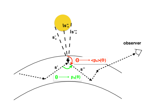
Figure 13: Photon trajectory simulation that shows the definition of $\theta$, $\Theta$ and the corresponding scattering phase functions in the radiative transfer model.

References

- Ackerman & Marley (2001) Ackerman, A.S. & Marley, M.S. 2001. Precipitating condensation clouds in substellar atmospheres. The Astrophysical Journal, 556, 872–884. doi: 10.1086/321540.
- Angerhausen et al. (2015) Angerhausen, D., DeLarme, E. & Morse, J.A., 2015. A comprehensive study of Kepler phase curves and secondary eclipses: Temperatures and albedos of confirmed Kepler giant planets. Publications of the Astronomical Society of Pacific, 127, 1113–1130. doi: 10.1086/683797.
- Barclay et al. (2012) Barclay, T., Huber, D., Rowe, J.F., Fortney, J.J., Morley, C.V., et al. 2012. Photometrically derived masses and radii of the planet and star in the TrES-2 system. The Astrophysical Journal, 761, id.53. doi: 10.1088/0004-637X/761/1/53.
- Barstow et al. (2017) Barstow, J.K., Aigrain, S., Irwin, P.G.J. & Sing, D.K. 2017. A consistent retrieval analysis of 10 hot Jupiters observed in transmission. The Astrophysical Journal, 834, id.50. doi: 10.3847/1538-4357/834/1/50.
- Borucki et al. (2003) Borucki, W.J., Koch, D.G., Lissauer, J.J., Basri, G.B., Caldwell, J.F., et al. 2003. The Kepler mission: a wide-field-of-view photometer designed to determine the frequency of Earth-size planets around solar-like stars. Proceedings of the SPIE, 4854, 129–140. doi: 10.1117/12.460266.
- Brown (2001) Brown, T.M. 2001. Transmission spectra as diagnostics of extrasolar giant planet atmospheres. The Astrophysical Journal, 553, 1006–1026. doi: 10.1086/320950.
- Budaj (2013) Budaj, J. Light-curve analysis of KIC 12557548b: an extrasolar planet with a comet-like tail. Astronomy & Astrophysics, 557, id.A72. doi: 10.1051/0004-6361/201220260.
- Budaj et al. (2015) Budaj, J., Kocifaj, M., Salmeron, R. & Hubeny, I. 2015. Tables of phase functions, opacities, albedos, equilibrium temperatures, and radiative accelerations of dust grains in exoplanets. Monthly Notices of the Royal Astronomical Society, 454, 2–27. doi: 10.1093/mnras/stv1711.
- Casagrande & VandenBerg (2014) Casagrande, L. & VandenBerg, D.A. 2014. Synthetic stellar photometry – I. General considerations and new transformations for broad-band systems. Monthly Notices of the Royal Astronomical Society, 444, 392–419. doi: 10.1093/mnras/stu1476.
- Chamberlain & Hunten (1987) Chamberlain, J.W. & Hunten, D.M. 1987. Theory of planetary atmospheres. An introduction to their physics and chemistry. International Geophysics Series, 36. Academic Press Inc., Orlando, FL, USA.
- Cubillos et al. (2017) Cubillos, P., Erkaev, N.V., Juvan, I., Fossati, L., Johnstone, C.P., et al. 2017. An overabundance of low-density Neptune-like planets. Monthly Notices of the Royal Astronomical Society, 466, 1868–1879. doi: 10.1093/mnras/stw3103.
- De Kok & Stam (2012) de Kok, R.J. & Stam, D.M. 2012. The influence of forward-scattered light in transmission measurements of (exo)planetary atmospheres. Icarus, 221, 517–524. doi: 10.1016/j.icarus.2012.08.020.
- Demory (2014) Demory, B.-O. 2014. The albedos of Kepler’s close-in super-Earths. The Astrophysical Journal Letters, 789, id.L20. doi: 10.1088/2041-8205/789/1/L20.
- Demory & Seager (2011) Demory, B.-O. & Seager, S. 2011. Lack of inflated radii for Kepler giant planet candidates receiving modest stellar irradiation. The Astrophysical Journal Supplement, 197, id.12. doi: 10.1088/0067-0049/197/1/12.
- Demory et al. (2013) Demory, B.-O., de Wit, J., Lewis, N., Fortney, J., Zsom, A. et al. 2013. Inference of inhomogeneous clouds in an exoplanet atmosphere. The Astrophysical Journal Letters, 776, id.L25. doi: 10.1088/2041-8205/776/2/L25.
- DeVore et al. (2016) DeVore, J., Rappaport, S., Sanchís-Ojeda, R., Hoffman, K. & Rowe, J. 2016. On the detection of non-transiting exoplanets with dusty tails. Monthly Notices of the Royal Astronomical Society, 461, 2453–2460. doi: 10.1093/mnras/stw1439.
- Esteves et al. (2015) Esteves, L.J., De Mooij, E.J.W. & Jayawardhana, R. Changing phases of alien worlds: Probing atmospheres of Kepler planets with high-precision photometry. The Astrophysical Journal, 804, id.150. doi: 10.1088/0004-637X/804/2/150.
- Faigler et al. (2013) Faigler, S., Tal-Or, L., Mazeh, T., Latham, D.W. & Buchhave, L.A. 2013. BEER analysis of Kepler and CoRoT light curves. I. Discovery of Kepler-76b: A Hot Jupiter with evidence for superrotation. The Astrophysical Journal, 771, id.26. doi: 10.1088/0004-637X/771/1/26.
- Fossati et al. (2017) Fossati, L., Erkaev, N.V., Lammer, H., Cubillos, P.E., Odert, P., et al. 2017. Aeronomical constraints to the minimum mass and maximum radius of hot low-mass planets. Astronomy & Astrophysics, 598, id.A90. doi: 10.1051/0004-6361/201629716.
- García Muñoz & Mills (2012) García Muñoz, A. & Mills, F.P. 2012. The June 2012 transit of Venus. Framework for interpretation of observations. Astronomy & Astrophysics, 547, id.A22, doi:10.1051/0004-6361/201219738.
- García Muñoz & Mills (2015) García Muñoz, A. & Mills, F.P. 2015. Pre-conditioned backward Monte Carlo solutions to radiative transport in planetary atmospheres. Fundamentals: Sampling of propagation directions in polarising media. Astronomy & Astrophysics, 573, id.A72, doi:10.1051/0004-6361/201424042.
- García Muñoz et al. (2014) García Muñoz, A., Pérez-Hoyos, S. & Sánchez-Lavega, A. 2014. Glory revealed in disk-integrated photometry of Venus. Astronomy & Astrophysics Letters, 566, id.L1, doi:10.1051/0004-6361/201423531.
- García Muñoz & Isaak (2015) García Muñoz, A. & Isaak, K.G. 2015. Probing exoplanet clouds with optical phase curves. Proceedings of the National Academy of Sciences, 112, 13461–13466. doi: 10.1073/pnas.1509135112.
- García Muñoz et al. (2012) García Muñoz, A., Zapatero Osorio, M.R., Barrena, R., Montañés-Rodríguez, P., Martín, E.L. & Pallé 2012. Glancing views of the Earth: From a lunar eclipse to an exoplanetary transit. The Astrophysical Journal, 755, id.103, doi:10.1088/0004-637X/755/2/103.
- García Muñoz et al. (2017) García Muñoz, A., Lavvas, P. & West, R.A. 2017. Titan brighter at twilight than in daylight. Nature Astronomy, 1, id.0114. doi:10.1038/s41550-017-0114.
- Han et al. (2014) Han, E., Wang, S.X., Wright, J.T., Feng, Y.K., Zhao, M., et al. 2014. Exoplanet Orbit Database. II. Updates to Exoplanets.org. Publications of the Astronomical Society of Pacific, 126, 827–837. doi: 10.1086/678447.
- Hansen & Travis (1974) Hansen, J.E. & Travis, L.D. 1974. Light scattering in planetary atmospheres. Space Science Reviews, 16, 527–610. doi: 10.1007/BF00168069.
- Helling & Fomins (2013) Helling, C. & Fomins, A. 2013. Modelling the formation of atmospheric dust in brown dwarfs and planetary atmospheres. Philosophical Transactions of the Royal Society A: Mathematical, Physical and Engineering Sciences, 371, 20110581. doi: 10.1098/rsta.2011.0581.
- Heng (2016) Heng, K. 2016. A cloudiness index for transiting exoplanets based on the sodium and potassium lines: Tentative evidence for hotter atmospheres being less cloudy at visible wavelengths. The Astrophysical Journal Letters, 826, id.L16. doi: 10.3847/2041-8205/826/1/L16.
- Shporer & Hu (2015) Shporer, A. & Hu, R. 2015. Studying atmosphere-dominated hot Jupiter Kepler phase curves: Evidence that inhomogeneous atmospheric reflection is common. The Astronomical Journal, 150, id.112. doi: 10.1088/0004-6256/150/4/112.
- Hubbard et al. (2001) Hubbard, W.B., Fortney, J.J., Lunine, J.I., Burrows, A., Sudarsky, D. & Pinto, P. 2001. Theory of extrasolar giant planet transits. The Astrophysical Journal, 560, 413–419. doi: 10.1086/322490.
- Hui & Seager (2002) Hui, L. & Seager, S. 2002. Atmospheric Lensing and Oblateness Effects during an Extrasolar Planetary Transit. The Astrophysical Journal, 572, 540–555, doi:10.1086/340017.
- Jenkins & Doyle (2003) Jenkins, J.M. & Doyle, L.R. Detecting reflected light from close-in extrasolar giant planets with the Kepler photometer. The Astrophysical Journal, 595, 429–445. doi: 10.1086/377165.
- Johnson & Christy (1974) Johnson, P.B. & Christy, R.W., 1974. Optical constants of transition metals: Ti, V, Cr, Mn, Fe, Co, Ni, and Pd. Physical Review B, 9, 5056–5070. doi: 10.1103/PhysRevB.9.5056.
- Karkoschka et al. (1997) Karkoschka, E. & Lorenz, R.D. 1997. Latitudinal variation of aerosol sizes inferred from Titan’s shadow. Icarus, 125, 369–379. doi: 10.1006/icar.1996.5621.
- Knutson et al. (2014) Knutson, H.A., Benneke, B., Deming, D. & Homeier, D. 2014. A featureless transmission spectrum for the Neptune-mass exoplanet GJ436b. Nature, 505, 66. doi: 10.1038/nature12887.
- Koike et al. (1995) Koike, C., Kaito, C., Yamamoto, T., Shivai, H., Kimura, S. & Suto, H. 1995. Extinction spectra of corundum in the wavelengths from UV to FIR. Icarus, 114, 203–214. doi: 10.1006/icar.1995.1055.
- Kreidberg et al. (2014) Kreidberg, L., Bean, J.L., Désert, J.-M., Benneke, B., Deming, D. et al. 2014. Clouds in the atmosphere of the super-Earth exoplanet GJ1214b. Nature, 505, 69. doi: 10.1038/nature12888.
- Lammer et al. (2016) Lammer, H., Erkaev, N.V., Fossati, L., Juvan, I., Odert, P., et al. 2016. Identifying the ‘true’ radius of the hot sub-Neptune CoRoT-24b by mass-loss modelling. Monthly Notices of the Royal Astronomical Society: Letters, 461, L62–L66. doi: 10.1093/mnrasl/slw095.
- Lavvas et al. (2010) Lavvas, P., Yelle, R.V. & Griffith, C.A. 2010. Titan’s vertical aerosol structure at the Huygens landing site: Constraints on particle size, density, charge, and refractive index. Icarus, 210, 832–842. doi: 10.1016/j.icarus.2010.07.025.
- Lavvas et al. (2013) Lavvas, P., Koskinen, T. & Yelle, R.V. 2013. Aerosol properties in exoplanet atmospheres. European Planetary Science Congress 2013, London, UK.
- Lavvas & Koskinen (2017) Lavvas, P., & Koskinen, T. 2017. Aerosol properties in the atmospheres of extrasolar giant planets. The Astrophysical Journal (In press). astroph: 2017arXiv170809257L.
- Lecavelier des Etangs et al. (2008) Lecavelier Des Etangs, A., Pont, F., Vidal-Madjar, A. & Sing, D. 2008. Rayleigh scattering in the transit spectrum of HD 189733b. Astronomy and Astrophysics, 481, L83–L86. doi: 10.1051/0004-6361:200809388.
- Lee et al. (2016) Lee, G., Dobbs-Dixon, I., Helling, C., Bognar, K. & Woitke, P. 2016. Dynamic mineral clouds on HD 189733b. I. 3D RHD with kinetic, non-equilibrium cloud formation. Astronomy & Astrophysics, 594, id.A48. doi: 10.1051/0004-6361/201628606.
- Loeb & Gaudi (2003) Loeb, A., & Gaudi, B.S. 2003. Periodic flux variability of stars due to the reflex Doppler effect induced by planetary companions. The Astrophysical Journal, 588, L117–L120. doi: 10.1086/375551.
- Marley et al. (1999) Marley, M.S., Gelino, C., Stephens, D., Lunine, J.I. & Freedman, R. 1999. Reflected Spectra and Albedos of Extrasolar Giant Planets. I. Clear and Cloudy Atmospheres. The Astrophysical Journal, 513, 879.
- Mislis & Hodgkin (2012) Mislis, D. & Hodgkin, S. 2012. A massive exoplanet candidate around KOI-13: independent confirmation by ellipsoidal variations. Monthly Notices of the Royal Astronomical Society, 422, 1512–1517.
- Misra & Meadows (2014) Misra, A.K. & Meadows, V.S. 2014. Discriminating between cloudy, hazy, and clear sky exoplanets using refraction. The Astrophysical Journal Letters, 795, id.L14, doi:10.1088/2041-8205/795/1/L14.
- Morley et al. (2012) Morley, C.V., Fortney, J.J., Marley, M.S., Visscher, C., Saumon, D. & Leggett, S.K. Neglected clouds in T and Y dwarf atmospheres. The Astrophysical Journal, 756, id.172. doi: 10.1088/0004-637X/756/2/172.
- Morris & Naftilan (1993) Morris, S.L. & Naftilan, S.A. 1993. The equations of ellipsoidal star variability applied to HR 8427. Astrophysical Journal, 419, 344–348. doi: 10.1086/173488.
- Parmentier et al. (2013) Parmentier, V., Showman, A.P. & Lian, Y. 2013. 3D mixing in hot Jupiters atmospheres. I. Application to the day/night cold trap in HD 209458b. Astronomy & Astrophysics, 558, id.A91. doi: 10.1051/0004-6361/201321132.
- Pérez-Hoyos et al. (2016) Pérez-Hoyos, S., Sanz-Requena, J.F., Sánchez-Lavega, A. & Irwin, P.G.J., Smith, A. 2016. Saturn’s tropospheric particles phase function and spatial distribution from Cassini ISS 2010-11 observations. Icarus, 277, 1–18. doi: 10.1016/j.icarus.2016.04.022.
- Placek et al. (2016) Placek, B., Knuth, K.H. & Angerhausen, D. 2016. Combining photometry from Kepler and TESS to improve short-period exoplanet characterization. Publications of the Astronomical Society of Pacific, 128, 074503. doi: 10.1088/1538-3873/128/965/074503.
- Rages et al. (1983) Rages, K., Pollack, J.B. & Smith, P.H. 1983. Size estimates of Titan’s aerosols based on Voyager high-phase-angle images. Journal of Geophysical Research, 88, 8721–8728. doi: 10.1029/JA088iA11p08721.
- Robinson (2017) Robinson, T.D. 2017. A theory of exoplanet transits with light scattering. The Astrophysical Journal, 836, id.236. doi: 10.3847/1538-4357/aa5ea8.
- Sánchez-Lavega et al. (2004) Sánchez-Lavega, A., Pérez-Hoyos, S. & Hueso, R. 2004. Clouds in planetary atmospheres: A useful application of the Clausius-Clapeyron equation. American Journal of Physics, 72, 767–774. doi: 10.1119/1.1645279.
- Seager et al. (2000) Seager, S., Whitney, B.A. & Sasselov, D.D. 2000. Photometric Light Curves and Polarization of Close-in Extrasolar Giant Planets. The Astrophysical Journal, 540, 504–520. doi: 10.1086/309292.
- Sheets & Deming (2014) Sheets, H.A. & Deming, D. 2014. Statistical Eclipses of Close-in Kepler Sub-Saturns. The Astrophysical Journal, 794, id.133. doi: 10.1088/0004-637X/794/2/133.
- Shporer (2017) Shporer, A. 2017. The astrophysics of visible-light orbital phase curves in the space age. Publications of the Astronomical Society of Pacific, 129, 072001. doi: 10.1088/1538-3873/aa7112.
- Sidis & Sari (2010) Sidis, O. & Sari, R. 2010. Transits of transparent planets-atmospheric lensing effects. The Astrophysical Journal, 720, 904–911. doi: 10.1088/0004-637X/720/1/904.
- Sing et al. (2016) Sing, D.K., Fortney, J.J., Nikolov, N., Wakeford, H.R., Kataria, T., et al. 2016. A continuum from clear to cloudy hot-Jupiter exoplanets without primordial water depletion. Nature, 529, 59. doi: 10.1038/nature16068.
- Spiegel et al. (2014) Spiegel, D.S., Fortney, J.J. & Sotin, C. 2014. Structure of exoplanets. Proceedings of the National Academy of Sciences, 111, 12622–12627. doi: 10.1073/pnas.1304206111.
- Stevenson (2016) Stevenson, K.B. Quantifying and predicting the presence of clouds in exoplanet atmospheres. The Astrophysical Journal Letters, 817, L16. doi: 10.3847/2041-8205/817/2/L16.
- Stevenson et al. (2016) Stevenson, K.B., Lewis, N.K., Bean, J.L., Beichman, C., Fraine, J., et al. Transiting exoplanet studies and community targets for JWST’s Early Release Science program. Publications of the Astronomical Society of Pacific, 128, 094401. doi: 10.1088/1538-3873/128/967/094401.
- Sudarsky et al. (2000) Sudarsky, D., Burrows, A. & Pinto, P. 2000. Albedo and reflection spectra of extrasolar giant planets. The Astrophysical Journal, 538, 885–903. doi: 10.1086/309160.
- Tomasko & Smith (1982) Tomasko, M.G. & Smith, P.H. 1982. Photometry and polarimetry of Titan – Pioneer 11 observations and their implications for aerosol properties. Icarus, 51, 65–95. doi: 10.1016/0019-1035(82)90030-6.
- Tomasko et al. (2008) Tomasko, M.G., Doose, L., Engel, S., Dafoe, L.E., West, R., et al. 2008. A model of Titan’s aerosols based on measurements made inside the atmosphere. PSS, 56, 669–707. doi: 10.1016/j.pss.2007.11.019.
- Tremblin et al. (2017) Tremblin, P., Chabrier, G., Mayne, N.J., Amundsen, D.S., Baraffe, I., et al. 2017. Advection of potential temperature in the atmosphere of irradiated exoplanets: a robust mechanism to explain radius inflation. arXiv:1704.05440.
- Wakeford & Sing (2015) Wakeford, H.R. & Sing, D.K., 2015. Transmission spectral properties of clouds for hot Jupiter exoplanets. Astronomy & Astrophysics, 573, id.A122. doi: 10.1051/0004-6361/201424207.
- West et al. (1983) West, R.A., Hart, H., Simmons, K.E., Hord, C.W., Esposito, L.W., et al., 1983. Voyager 2 photopolarimeter observations of Titan. Journal of Geophysical Research, 88, 8699–8708. doi: 10.1029/JA088iA11p08699.
- West & Smith (1991) West, R.A. & Smith, P.H. 1991. Evidence for aggregate particles in the atmospheres of Titan and Jupiter. Icarus, 90, 330–333. doi: 10.1016/0019-1035(91)90113-8.