MARXS: A modular software to ray-trace X-ray instrumention

Abstract

To obtain the best possible scientific result, astronomers must understand the properties of the available instrumentation well. This is important both when designing new instruments and when using existing instruments close to the limits of their specified capabilities or beyond. Ray-tracing is a technique for numerical simulations where the path of many light rays is followed through the system to understand how individual system components influence the observed properties, such as the shape of the point-spread-function (PSF). In instrument design, such simulations can be used to optimize the performance. For observations with existing instruments this helps to discern instrumental artefacts from a true signal. Here, we describe MARXS, a new python package designed to simulate X-ray instruments on satellites and sounding rockets. MARXS uses probability tracking of photons and has polarimetric capabilities.

1 Introduction

Astronomical observations rely on increasingly complex instruments always pushing the boundaries in spatial and spectral resolution. Simulation software is an important tool to help astronomers and engineers to design and operate these instruments, to propose and plan observations, and to analyze data to extract scientific results.

Depending on the application, simulations with different levels of detail are needed. For example, to estimate if two close sources seen by one instrument will also be resolved by another, it might be sufficient to convolve an image with the point-spread-function (PSF) of the second instrument. On the other hand, for instruments where the PSF is strongly dependent on the wavelength, where the PSF changes significantly over the field-of-view (FOV), or where the pointing direction changes within an observation (e.g. due to dithering), more complex simulation tools are required. One approach is to perform a geometrical ray-trace simulation, where rays are propagated through all components of the instrument. The simulation starts at some position $\vec{r}_{0}$ (typically chosen in the aperture plane) with a ray direction $\vec{d}_{0}$ (parallel to the optical axis of the telescope for on-axis sources). The simulation follows the ray and calculates where it next intersects an element of the instrument, e.g. it might hit a mirror surface at position $\vec{r}_{1}=\vec{r}_{0}+\lambda\vec{d}_{0}$. At this point, the new propagation direction $\vec{d}_{1}$ of the ray is chosen. For a mirror surface, this depends on the angle of incidence, but other optical elements such as diffraction gratings or polarizing filters might take other ray properties into account. In this way the simulation tracks the ray until it hits (or misses) the detector. The process is repeated for many rays starting at different $r_{0}$ and with different wavelengths and polarization vectors. In the end, the list of rays can be analyzed. For example, the position of intersection with the detector can be binned into a 2-D histogram to yield a simulated detector image. Ray-tracing as a technique is particularly well-suited to track the influence of aberrations such as coma and astigmatism, to predict the shadows cast by support structures and baffles, and to analyze the effect of gratings and detectors that are flat, while the analytically derived focal plane would require them to be curved.

Ray-tracing helps with the design of instruments (e.g. Willingale et al., 2014) when decisions about the placement of the instrument components are made, it helps to predict the performance of instruments, can be used to derive calibration products such as the instrumental line width of a spectrograph (Flanagan et al., 2000), and finally it can be used predict the instrumental signal for a specific astrophysical model to facilitate proposal writing or for comparison to observed data (e.g. Zu Hone et al., 2009).

To give a few examples how ray-tracing helps to enable specific scientific results, the MARX software (Davis et al., 2012) can generate a model of the PSF of the Chandra observatory at a specific position in the focal plane for the specific dither pattern and source spectrum of the observation in question. Using this, Russell et al. (2012) are able to model the wings of the PSF in the quasar PKS 1229-021 and detect an extended emission component from the cool-core cluster surrounding it and similarly Wu et al. (2017) find extended emission around the radio galaxy C 41.17. In a similar use the ACISExtract package (Broos et al., 2010) runs a MARX simulation for every detected point source to determine the appropriate extraction radius. The resulting flux scale is directly tied to the accuracy of the ray-trace simulation. ACISExtract is often used in the analysis of stellar clusters (e.g. Kuhn et al., 2013). Miller et al. (2014) used MARX simulations to estimate the uncertainty in the zero-point of the velocity scale in a dispersion grating to verify the redshift of absorption lines observed in the transient X-ray binary MAXI J1305-704.

In this paper, we present a new python software package called MARXS (Multi-Architecture-Raytrace-Xraymission-Simulator) that derives many ideas from the Chandra MARX code. Previous ray-trace codes are often either specific to a single X-ray mission like MARX for Chandra or SciSim (Gabriel et al., 2005) for XMM-Newton or they are not easily available to all potential users of a mission because they rely on expensive commercial packages or are implemented in very specialized programming languages like MT_RAYOR (Westergaard, 2011) which is implemented in Yorick and used for NuStar and ASTROSAT. Our new MARXS package is written in Python and distributed under version 3 of the GNU Public license (GPL). MARXS provides generic implementations of elements commonly found in X-ray instruments which can be combined as needed to setup simulations for a wide range of use cases.

In section 2 we explain the design principles and capabilities of the MARXS code. In section 3 we show examples of using it. We end with a short summary in section 4. This paper describes version 1.1 of MARXS (Günther et al., 2017). Development continues on github.

Note to astroph readers: This article was accepted by AJ and the journal will host interactive versions of figures 1 and 3 after publication. In the meantime, interactive versions of those figures can also be found in the documentation of the MARXS software. The specific url is given in the figure caption.

2 Design and capabilities

This section explains aspects of the software design and mentions some of the modules and classes in MARXS. Module names, classes and other Python code are written monospaced. This section is not intended to replace the MARXS documentation where further details and code examples can be found.

MARXS contains classes for X-ray sources (in module marxs.source) and optical elements such as mirrors, baffles, diffraction gratings, and detectors (marxs.optics). The marxs.simulator modules contains classes that help grouping optical elements, e.g. different CCDs that make up one camera. There are supporting modules to help with the instrument design in marxs.design to calculate the proper placement of diffraction gratings and detectors on a torus for a Rowland spectrometer (see e.g. Beuermann et al., 1978). The display of results is handled in (marxs.visualization), as well as utility modules for mathematics.

2.1 Order of elements in the simulation

MARXS visits elements sequentially. After a ray passes (and potentially interacts with) element $i$, MARXS tests if the ray interacts with element $i+1$. The ray never returns to element $i$. This approach reduces the number of intersection tests that need to be calculated per ray-trace, but it requires an A-priory knowledge about the order of elements that a ray might intersect with. This means that MARXS is of limited use to estimate the scattered light in an instrument, because it cannot handle rays that bounce back to “earlier” elements.

2.2 Units and coordinate systems

MARXS uses homogeneous coordinates, which describe position and direction in a 4 dimensional coordinate space [$x$, $y$, $z$, $w$]. For example, [3,0,0,1] describes a point at $x/w=3$, $y/w=0$, and $z/w=0$. The vector [3,0,0,0] describes a point at infinity, because $x/w$=3/0. Points at infinity can be thought of a “direction vector”, so that a [1,0,0,0], [2,0,0,0] or [3,0,0,0] would all describe a vector parallel to the x-axis. In homogeneous coordinates, rotation, zoom, and translations together can be described by a [4,4] matrix and several of these operations can be chained simply by multiplying the matrices.

Every optical element in MARXS has such a [4,4] matrix associated with it in an attribute called pos4d. We experimented with astropy’s unit system (Astropy Collaboration et al., 2013), but found that it added significant overhead. Thus, dimensional numbers are represented as simple floating point numbers in the code, and by convention we assume all spatial units to be given in mm and all energies in keV. Use of astropy’s units system for input with automatic conversion to these base units internally is planned for a future version.

2.3 Rays and photons

The fundamental unit of ray-tracing is a single “ray”, which can be interpreted as a wave package of many photons or as a single photon. Most X-ray detectors are photon counting, thus it is convenient to identify each ray with a single photon in this case. MARXS generates a list of photons, which is stored in an astropy.table.Table object (Astropy Collaboration et al., 2013). This object holds numpy arrays and associated metadata. It also provides the capability of saving data in fits and other formats, while at the same time, mathematical operations such as dot and cross-products can be performed efficiently on the numpy arrays.

2.4 No simulation of microphysics

Currently, MARXS does not provide classes to calculate the result of an interaction with an element from the properties of the material. Instead, it requires the user to provide look-up tables for quantities such as reflection probabilities or grating efficiencies. Alternatively, the user can supply code to calculate these quantities from first principles.

As an example, the MARXS class FlatGrating does not calculate the diffraction probability in every order from the optical constants of the materials that make up the gratings and the dimensions of individual bars; instead, it uses tabulated diffraction efficiencies from a file and assigns a diffraction order to every ray based on those numbers, so that the dispersion angle can be calculated from the grating constant and the grating equation. This approach allows the flexibility to use either theoretical grating efficiencies pre-calculated by some other program or interpolate experimentally determined values.

2.5 Polarization

MARXS supports polarization ray-tracing, but the proper treatment of polarization is not yet implemented for all components of MARXS.

The polarization of each ray is represented as a 3d-vector and uses matrices to move this vector in space. As an extension of the 2-d Jones calculus, this method is particularly suited for light paths that are not all parallel (Chipman, 1992). See Yun et al. (2011) and Yun (2011) for details on polarization ray tracing and the derivation of the relevant matrices.

This mechanism can handle both linear and circular polarized light. However, the light sources currently included in MARXS only support linear polarization.

2.6 Sources and apertures

The module marxs.sources provides several classes for point sources both in the laboratory and on the sky. There are also a few classes for spatially extended celestial sources such as circle, disk, or Gaussian luminosity distribution. All sources allow great freedom to specify spectral properties, polarizations, and timing behavior through keywords. For astrophysical sources, the telescope pointing must be specified to transform the origin of the photons in sky coordinates to a direction in the instrument coordinate system. The aperture class then assigns the ray a randomized initial position in the instrument frame. This random sampling of the aperture means that simulations need to be run with a number of rays that is sufficient to sample the aperture.

Laboratory sources generate rays in the coordinate system of the experiment and no further pointing or aperture is required.

2.7 Parts and pieces

MARXS provides a range of generic optical elements such as mirrors, gratings, filters, and detectors in marxs.optics. Each object is initialized with a 4-d matrix that sets positions and orientation compared relative to the global coordinate system, and the size of each element. Additional properties such as pixel size or grating constant are passed in as keywords. Some of these elements are demonstrated in the examples below.

The optical elements are laid out in a hierarchy based on inheritance. This makes is easy to add new elements, since they can inherit most of their functionality from existing base classes, so that only little new code has to be written.

2.8 Probability tracking

Many elements in an X-ray optics absorb photons. One way to treat this in a Monte-Carlo ray-trace is to draw a random number and decide for each ray if it should be deleted from the list of rays or propagated further. However, in the setup of MARXS it is much easier to operate on a photon list of fixed size. Thus, each photon in MARXS has a probability associated with it. At the source, the value $1.0$ is assigned and in any absorbing element this number is decreased to track the probability that the photon is still present. For example, a photon reflected by a mirror with 80% reflection efficiency and passing through an optical blocking filter with 90% X-ray transmission, will have $p=0.8*0.9=0.72$.

2.9 Visualization

MARXS photons lists are just astropy tables, and as such they have built-in capability to be written to a variety of file formats, including fits tables. Thus, any standard astronomy software can be used to analyze simulation results. For example, binning the x and y coordinates of the rays on the detector yields a detector image. Furthermore, MARXS also provides several ways to pass the coordinates of the instrument components and of the rays to 3-d visualization tools. Currently supported are Mayavi (Ramachandran & Varoquaux, 2011), a Python library, and three.js, a javascript library. Both of them make use of the OpenGL standard, so that the 3-dimensional rendering is done in the graphics card of the computer, making fluid animations of instrument designs with hundreds of mirror modules, gratings and detectors and thousands of photon pathways possible. In particular, Mayavi can export the data to the x3d format, which is particularly suited for inclusion in presentations and publications (Vogt et al., 2016). Figures 1 and 3 are produced in this way and are fully interactive in the online version of this article.

2.10 Verification

MARXS employs continuous integration with a few hundred unit tests to reduce the risk of unintended regressions. Test cases include verification that all classes adhere to the common interface (e.g. all optical elements can be called with a photon list as argument), physical boundary conditions are preserved (e.g. the polarization vectors are always perpendicular to the directions of the ray), and, where available, analytical test cases are correctly simulated (e.g. the grating equation for a diffraction grating).

3 Examples

In this section, we show two examples of experiments that can be easily simulated with MARXS. Both examples are covered in more detail in the documentation of MARXS where the full source code is given.

3.1 The benefit of sub-aperturing

Collimation of X-rays typically requires double reflection of a mirror shell at grazing incidence. When they leave the mirror, photons are distributed on the surface of a cone where the focal point of the mirror is the tip of the cone. In some situations, it can be beneficial to use only a fraction of the mirror. This is called sub-aperturing. In this example, we simulate an instrument with sub-aperturing. Instrument parameters are inspired by the Chandra/HETG (Canizares et al., 2005), but optical elements are much bigger, so that we can explore what effect large diffraction gratings and detectors have. On the one hand, using larger elements reduces the area covered by support structures and thus increases the throughput of the telescope; on the other hand, large, flat elements deviate more from the analytic curved surface where gratings and detectors should be placed in a Rowland geometry.

In this simulation, the focal length is 11 m, the grating constant is 200 nm, the gratings are 160 mm on each side, and detectors are rectangular with $100\times 40$ mm². Figure 1 shows a ray-trace for a source on axis with a monochromatic flux of 1 keV. The entrance aperture is a narrow ring in the blue, partially transparent plate. Rays are placed in this aperture and propagated parallel to the optical axis. The mirror is approximated with a simple model: All photons passing the gray plate in the figure are focused to the focal point, then some random scatter is added. Figure errors, surface roughness, and particulates scatter X-rays by a larger angle in the plane of incidence than perpendicular to it (Cash, 1987). Thus, the scatter is typically larger in the plane of incidence than perpendicular to it (O’dell et al., 1993; Collon et al., 2015). In this simulation, we explore the case where in-plane scatter is a few times larger than scatter perpendicular to the plane of reflection. Transmission gratings (red, green, and blue) and detectors (yellow) are placed on the Rowland Torus, a section of which is shown as a partially transparent, red surface. In the figure, the detectors are very hard to see, because they are only a few cm large and are located several meters from the front of the telescope. This difference in scale is often found in X-ray telescopes and thus it is very useful to be able to interactively pan and zoom in the figure - this is possible in the electronic version of this article.

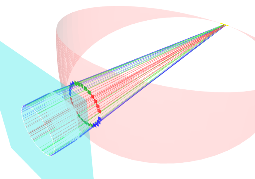
Figure 1: A simulation to study sub-aperturing. The entrance aperture is a narrow ring in the blue plane. The gray plane indicates the simplified mirror model. Diffraction gratings (red, green, and blue) as well as detectors (yellow, in the top right corner) are placed in the Rowland Torus (red surface). Lines are 1 keV rays, which are colored to match the grating they pass through. For visibility only a few hundred rays are shown. An interactive version of this figure is available at https://marxs.readthedocs.io/en/latest/visualization.html (about 2/3 down the page).

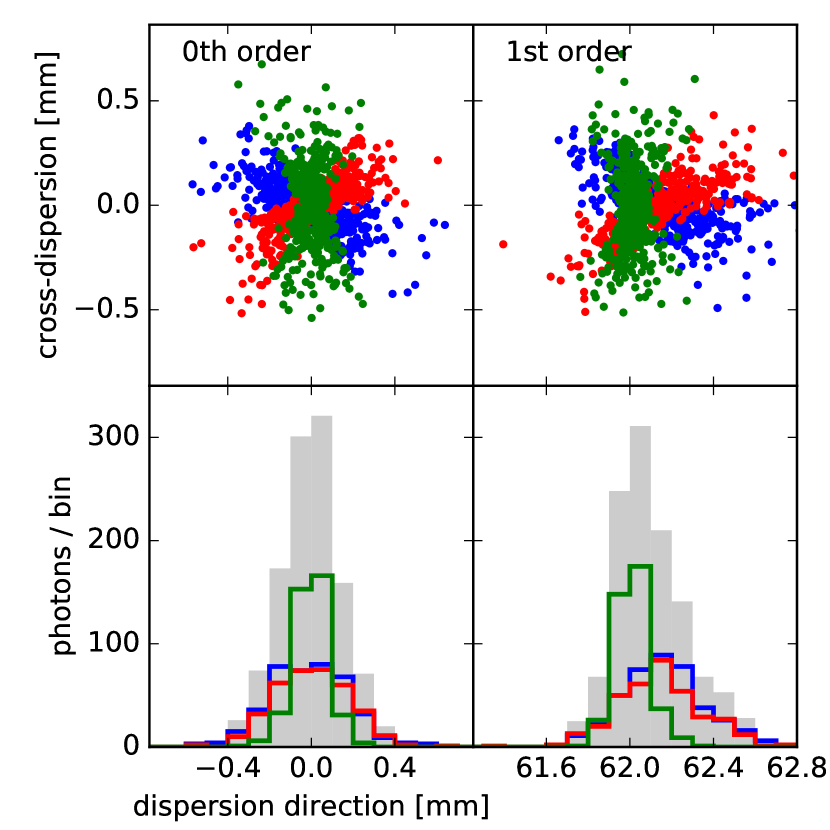
Figure 2: top: Photon positions on the detector bottom: Histogram of the distribution in dispersion direction. Colors match the color of the dots in the top row and respective diffraction gratings in figure 1. The gray blocks show the summed histogram. left: zeroth order. right: first order. Note that this figure displays a simulation with a larger number of photons than figure 1.

Rays are colored according to the grating they pass through and they are diffracted with equal probability into the grating orders -1, 0, and +1. Figure 2 also shows the detector image of the zeroth and first order.

The PSF in zeroth order is rotationally symmetric, but if photons are selected through a sub-aperture, the PSF narrows considerably in one direction. In the plot, the photons shown in green are narrow in the dispersion direction and thus they give a sharper feature in the first order than the other photons, leading to a spectrograph with increased resolving power. By varying several parameters of the simulation such as the size of gratings and detectors, MARXS can also be used to understand the asymmetric shape of the first-order PSF, which is due to a combination of aberration and the finite-size of the large gratings, but a detailed discussion is beyond the scope of this simple usage example.

3.2 The effect of polarization

This example reproduces a setup in a laboratory X-ray beamline, where X-ray polarization using multi-layer mirrors is studied (Marshall et al., 2013). The experiment consists of four elements (figure 3): First, there is an X-ray source that can be operated with a range of anodes to control the spectrum of the source. To simplify matters for the simulation, we will assume monochromatic light here. The source has a small opening aperture and shines on a multi-layer mirror (green) with an incidence angle of 45^∘, which matches the Brewster angle. This angle is defined as the angle where p-polarized light is perfectly transmitted and only s-polarized light (polarization direction perpendicular to the plane of reflection) will be reflected. When unpolarized light arrives at the mirror at the Brewster angle, the reflected light is thus 100% polarized. X-rays transmitted through the reflecting surface will be absorbed by the lower layers of the mirror substrate and the holder and are lost, we only track the reflected light. Multilayer coatings can reflect a few percent of the incoming X-rays. Together, the source and this first mirror can be thought of as a “source of polarized X-rays”. From the first mirror, X-rays are directed onto a second mirror (blue), which they reach again at the Brewster angle, and finally a detector (yellow). Source and first mirror can be rotated with respect to the second mirror, changing the polarization angle of the light that reaches the second mirror. If the incoming light is s-polarized with respect to the second mirror, it will reflect a fraction of the light to the detector. When source and first mirror are rotated by 90^∘ the polarization vector of the photons will be parallel to the plane of reflection with the second mirror, and no light is reflected. Figure 3 shows the setup for several different positions of source and first mirror. Figure 4 shows how the intensity of the detected light changes with the rotation angle. Marshall et al. (2013) perform this experiment in the laboratory albeit with different physical dimensions. In the figure, we compare the normalized simulated flux with the experimental results and find an excellent agreement. The statistical errors on the data are smaller than the plot symbols, but there is an additional systematic error in the measurement of the rotation angle (x-axis of the plot). The size of this error is not quantified in Marshall et al. (2013), but large enough to explain the differences between simulated and measured data (Marshall, personal communication).

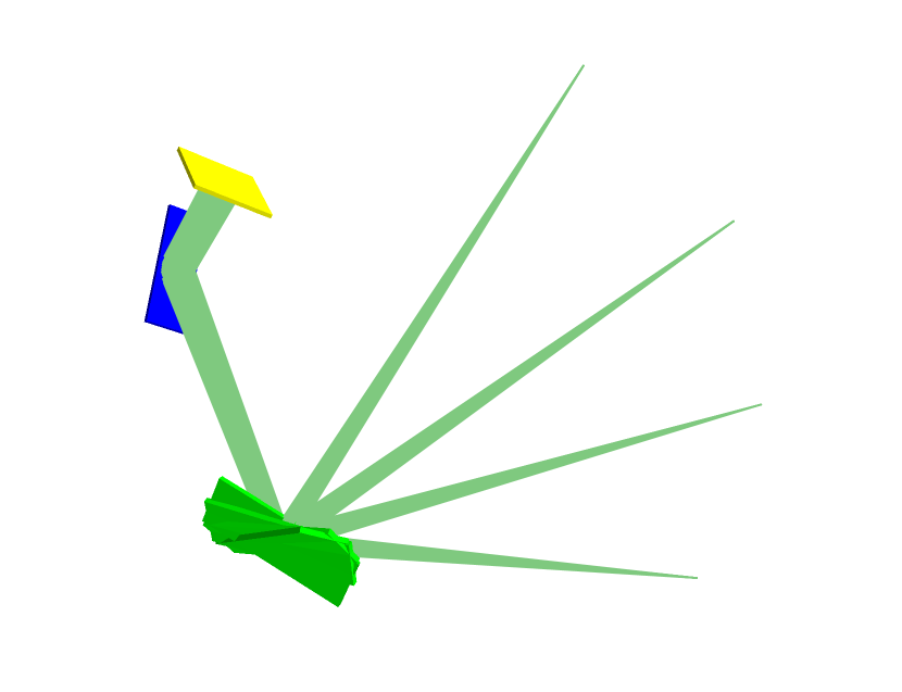
Figure 3: Setup of the polarization experiment. The components are two mirrors (green and blue) and the detector (yellow). Simulated rays are shown in green, the light source is at the tip of the cone. The figure shows four positions for the lightsource and the corresponding rotation of the green mirror. The green mirror is positioned in such a way that all rays reach the blue mirror and the detector for every rotation angle of the source. An interactive version of this figure is available at https://marxs.readthedocs.io/en/latest/examples.html (about 2/3 down the page).

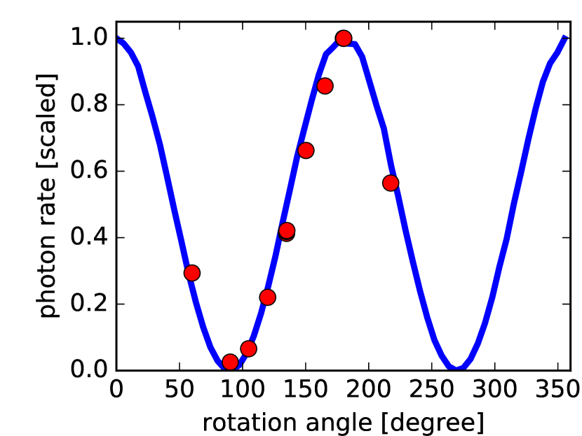
Figure 4: Photon fluxes for a simulation for different rotation angles of source and green mirror. The data points are taken from Marshall et al. (2013) where this setup is tested in the lab (physical dimensions for the mirrors and the distance between the elements differ from the simulation). Statistical

error bars are smaller than the plot symbols.

3.3 Mission proposals

MARXS has already been used in Günther et al. (2016) to demonstrate that a design based on critical-angle transmission gratings (Heilmann et al., 2015) can achieve a spectral resolving power of several thousand with very modest requirements on the grating alignment using the baseline design for Lynx (Gaskin et al., 2015) and ARCUS (Smith et al., 2014). ARCUS is currently proposed as an explorer mission to NASA and Lynx is one of the studies for NASA’s 2020 decadal survey. Particularly for ARCUS, simulations with MARXS were instrumental to define the optical layout.

The capability for polarization ray-tracing allowed refinements of the optical design for the REDSoX mission (Marshal et al., in prep), a proposed sounding rocket experiment for a soft X-ray polarimeter.

4 Summary

MARXS is a new ray-tracing code in python that is designed to simulate the performance of X-ray instrumentation on the ground and in space. It includes modules for common elements such as mirrors, dispersion gratings, and detectors. MARXS tracks the probability of a photon to travel along its pathway without absorption by the optical elements it passes. Polarization is taken into account where appropriate. We show the use of MARXS to study sub-aperturing, to replicate the laboratory setup of an X-ray beamline, and to design future instrumentation.

References

- Astropy Collaboration et al. (2013) Astropy Collaboration, Robitaille, T. P., Tollerud, E. J., et al. 2013, A&A, 558, A33
- Beuermann et al. (1978) Beuermann, K. P., Bräuninger, H., & Trümper, J. 1978, Appl. Opt., 17, 2304. http://ao.osa.org/abstract.cfm?URI=ao-17-15-2304
- Broos et al. (2010) Broos, P. S., Townsley, L. K., Feigelson, E. D., et al. 2010, ApJ, 714, 1582
- Canizares et al. (2005) Canizares, C. R., Davis, J. E., Dewey, D., et al. 2005, PASP, 117, 1144
- Cash (1987) Cash, W. 1987, Appl. Opt., 26, 2915. http://ao.osa.org/abstract.cfm?URI=ao-26-14-2915
- Chipman (1992) Chipman, R. A. 1992, in Proc. SPIE, Vol. 1746, Polarization Analysis and Measurement, ed. D. H. Goldstein & R. A. Chipman, 62–75
- Collon et al. (2015) Collon, M. J., Vacanti, G., Günther, R., et al. 2015, in Proc. SPIE, Vol. 9603, Society of Photo-Optical Instrumentation Engineers (SPIE) Conference Series, 96030K
- Davis et al. (2012) Davis, J. E., Bautz, M. W., Dewey, D., et al. 2012, in Proc. SPIE, Vol. 8443, Space Telescopes and Instrumentation 2012: Ultraviolet to Gamma Ray, 84431A
- Flanagan et al. (2000) Flanagan, K. A., Markert, T. H., Davis, J. E., et al. 2000, in Proc. SPIE, Vol. 4140, X-Ray and Gamma-Ray Instrumentation for Astronomy XI, ed. K. A. Flanagan & O. H. Siegmund, 559–572
- Gabriel et al. (2005) Gabriel, C., Ibarra Ibaibarriaga, A., & Hoar, J. 2005, in Proc. SPIE, Vol. 5898, UV, X-Ray, and Gamma-Ray Space Instrumentation for Astronomy XIV, ed. O. H. W. Siegmund, 450–459
- Gaskin et al. (2015) Gaskin, J. A., Weisskopf, M. C., Vikhlinin, A., et al. 2015, in Proc. SPIE, Vol. 9601, UV, X-Ray, and Gamma-Ray Space Instrumentation for Astronomy XIX, 96010J
- Günther et al. (2016) Günther, H. M., Bautz, M. W., Heilmann, R. K., et al. 2016, in Proc. SPIE, Vol. 9905, Society of Photo-Optical Instrumentation Engineers (SPIE) Conference Series, 990556
- Günther et al. (2017) Günther, H. M., Frost, J., , & Theriault-Shay, A. 2017, Chandra-MARX/marxs: v1.1, Zenodo, doi:10.5281/zenodo.829911. https://doi.org/10.5281/zenodo.829911
- Heilmann et al. (2015) Heilmann, R. K., Bruccoleri, A. R., & Schattenburg, M. L. 2015, in Proc. SPIE, Vol. 9603, Society of Photo-Optical Instrumentation Engineers (SPIE) Conference Series, 960314
- Kuhn et al. (2013) Kuhn, M. A., Getman, K. V., Broos, P. S., Townsley, L. K., & Feigelson, E. D. 2013, ApJS, 209, 27
- Marshall et al. (2013) Marshall, H. L., Schulz, N. S., Remlinger, B., et al. 2013, in Proc. SPIE, Vol. 8861, Optics for EUV, X-Ray, and Gamma-Ray Astronomy VI, 88611D
- Miller et al. (2014) Miller, J. M., Raymond, J., Kallman, T. R., et al. 2014, ApJ, 788, 53
- O’dell et al. (1993) O’dell, S. L., Elsner, R. F., Kolodziejeczak, J. J., et al. 1993, in Proc. SPIE, Vol. 1742, Multilayer and Grazing Incidence X-Ray/EUV Optics for Astronomy and Projection Lithography, ed. R. B. Hoover & A. B. C. Walker, Jr., 171–182
- Ramachandran & Varoquaux (2011) Ramachandran, P., & Varoquaux, G. 2011, Computing in Science & Engineering, 13, 40
- Russell et al. (2012) Russell, H. R., Fabian, A. C., Taylor, G. B., et al. 2012, MNRAS, 422, 590
- Smith et al. (2014) Smith, R. K., Ackermann, M., Allured, R., et al. 2014, in Proc. SPIE, Vol. 9144, Space Telescopes and Instrumentation 2014: Ultraviolet to Gamma Ray, 91444Y–91444Y–12. http://dx.doi.org/10.1117/12.2062671
- van der Walt et al. (2011) van der Walt, S., Colbert, S. C., & Varoquaux, G. 2011, Computing in Science & Engineering, 13, 22. http://aip.scitation.org/doi/abs/10.1109/MCSE.2011.37
- Vogt et al. (2016) Vogt, F. P. A., Owen, C. I., Verdes-Montenegro, L., & Borthakur, S. 2016, ApJ, 818, 115
- Westergaard (2011) Westergaard, N. J. 2011, in Proc. SPIE, Vol. 8147, Society of Photo-Optical Instrumentation Engineers (SPIE) Conference Series, 81470Y
- Willingale et al. (2014) Willingale, R., Pareschi, G., Christensen, F., et al. 2014, in Proc. SPIE, Vol. 9144, Space Telescopes and Instrumentation 2014: Ultraviolet to Gamma Ray, 91442E
- Wu et al. (2017) Wu, J., Ghisellini, G., Hodges-Kluck, E., et al. 2017, MNRAS, 468, 109
- Yun (2011) Yun, G. 2011, Polarization Ray Tracing, The University of Arizona. http://hdl.handle.net/10150/202979
- Yun et al. (2011) Yun, G., Crabtree, K., & Chipman, R. A. 2011, Appl. Opt., 50, 2855. http://ao.osa.org/abstract.cfm?URI=ao-50-18-2855
- Zu Hone et al. (2009) Zu Hone, J. A., Ricker, P. M., Lamb, D. Q., & Karen Yang, H.-Y. 2009, ApJ, 699, 1004