On a Minkowski geometric flow in the plane: evolution of curves with lack of scale invariance

Abstract

We consider a planar geometric flow in which the normal velocity is a nonlocal variant of the curvature. The flow is not scaling invariant and in fact has different behaviors at different spatial scales, thus producing phenomena that are different with respect to both the classical mean curvature flow and the fractional mean curvature flow.

In particular, we give examples of neckpinch singularity formation, and we discuss convexity properties of the evolution.

We also take into account traveling waves for this geometric flow, showing that a new family of $C^{1,1}$ and convex traveling sets arises in this setting.

1 Introduction

In this paper we consider a planar geometric flow and we discuss its basic properties, such as singularity formation, convexity preserving and existence of traveling waves. This geometric flow is the gradient flow of a nonlocal perimeter which is not invariant under scaling, therefore the evolution of a set presents different properties at different scales (in this, the flow has natural applications in image digitalization, especially when tiny details have to be preserved after denoising, as in the case of fingerprints storage).

The mathematical framework in which we work is the following. For any set $E\subset\mathbb{R}^{2}$ with $C^{2}$ boundary and any $x\in\partial E$ we denote by $B_{r,x}^{\mathrm{ext}}$ the ball of radius $r>0$ which is locally externally tangent to $\partial E$ at $x$ (that is, $B_{r,x}^{\mathrm{ext}}:=B_{r}(x+r\nu_{E}(x))$, where $\nu_{E}$ is the external unit normal).

Similarly, we denote by $B_{r,x}^{\mathrm{int}}$ the ball of radius $r$ which is locally internally tangent to $\partial E$ at $x$ (that is, $B_{r,x}^{\mathrm{int}}:=B_{r}(x-r\nu_{E}(x))$).

We also denote by ${\kappa(E,x)}$ the curvature of $\partial E$ at the point $x$. Then we define the $r$-curvature of $\partial E$ at $x$ as

$$\begin{split}&\kappa_{r}(E,x):=\kappa_{r}^{+}(E,x)+\kappa_{r}^{-}(E,x),\\ {\mbox{where }}\quad&\kappa_{r}^{+}(E,x):=\left\{\begin{matrix}\displaystyle\frac{\kappa(E,x)}{2}+\frac{1}{2r}&{\mbox{if }}B_{r,x}^{\mathrm{ext}}\subseteq\mathbb{R}^{2}\setminus E,\\ 0&{\mbox{ otherwise,}}\end{matrix}\right.\\ {\mbox{and }}\quad&\kappa_{r}^{-}(E,x):=\left\{\begin{matrix}\displaystyle\frac{\kappa(E,x)}{2}-\frac{1}{2r}&{\mbox{if }}B_{r,x}^{\mathrm{int}}\subseteq E,\\ 0&{\mbox{ otherwise,}}\end{matrix}\right.\end{split}$$ (1.1)

see formulas (2.10), (2.11) and (2.12) and Lemma 2.1 in [MR3023439].

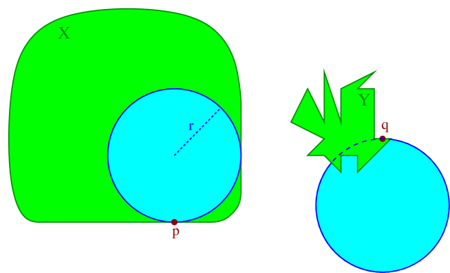
Figure 1: Examples for $\kappa_{r}$.

We point out that, differently from the case of the classical curvature, there are sets with $C^{2}$ boundary for which $\kappa_{r}$ is not continuous (see for instance Figure 1, in which the set $X$ has $C^{2}$ boundary, but $\kappa_{r}$ jumps from $0$ to $\frac{1}{2r}$ at the point $p$, and the set $Y$, which is not $C^{2}$ in an $r$-neighborhood of $q$, but for which $\kappa_{r}$ is identically zero in such a neighborhood).

Fixed $r\in(0,1]$, we consider here the geometric flow with normal velocity equal to $\kappa_{r}$, namely if $E_{t}$ denotes the evolution of a set $E\subset\mathbb{R}^{2}$ and $x_{t}\in\partial E_{t}$, we study the equation

$$\partial_{t}x_{t}\cdot\nu_{E_{t}}(x_{t})=-\kappa_{r}(E_{t},x_{t}).$$ (1.2)

The existence of a solution, in the viscosity sense, of this nonlocal geometric problem has been established in [MR3023439, MR3156889, MR3401008]. The geometric equation in (1.2) can be seen as the gradient flow of a nonlocal functional built by the approximated Minkowski content, see [MR2655948, 2017arXiv170403195C].

Of course, the quantity $r$ in (1.2) plays a special role, producing a discontinuity in the velocity field of the geometric flow and detecting special features “at a small scale”. Therefore, to perform our analysis, we consider a special class of sets, which are “slim” (or “pudgy”) with respect to such a scale.

Definition 1.1.

A set $E\subseteq\mathbb{R}^{2}$ is called “$r$-pudgy” if it contains a ball of radius $r$. Otherwise, it is called “$r$-slim”.

A particular case of $r$-slim sets is given by those which have the “diameter in one direction” that is less than $r$:

Definition 1.2.

A set $E\subseteq\mathbb{R}^{2}$ is called “$r$-thin” if, after a rigid motion, it holds that $E\subseteq\mathbb{R}\times(-\rho,\rho)$, with $\rho\in(0,r)$.

The first problem that we take into account is the possible formation of neckpinch singularities in the flow defined by (1.2). We recall that in the classical mean curvature flow (or curve shortening flow), Grayson’s Theorem [MR906392] gives that no singularity occurs in the plane, and, in fact, the initial set becomes convex and then shrinks smoothly towards a point. Interestingly, this result is not true for the planar nonlocal geometric flow in (1.2) and neckpinch singularities occur.

We construct two families of counterexamples, one for $r$-thin and one for $r$-pudgy sets. The first result is the following:

Theorem 1.3 (Neckpinch singularity formation for $r$-thin sets).

Assume that $r$ is sufficiently small. Then, there exists an $r$-thin connected set $E\subset(-1,1)\times\left(-\frac{r}{2},\frac{r}{2}\right)$, with $C^{\infty}$ boundary and such that any viscosity solution of the $r$-mean curvature flow (1.2) starting from $E$ does not shrink to a point (and any viscosity evolution of $E$ becomes disconnected).

Such $E$ has a “narrow dumbbell shape” in the sense that it is obtained by gluing two balls of radius $r/4$ with a neck contained in $(-1,1)\times\left(-\frac{r}{100},\frac{r}{100}\right)$.

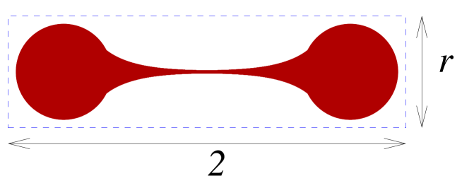
Figure 2: The set in Theorem 1.3.

The idea of the set constructed in Theorem 1.3 is depicted in Figure 2. Roughly speaking, the vertical trapping of the set will force the inner $r$-curvatures $\kappa^{-}_{r}$ in (1.1) to vanish, while the outer $r$-curvatures $\kappa^{+}_{r}$ will make the neck of the set shrink faster than the two balls on the side, thus producing the singularity.

In a sense, the example in Theorem 1.3 is quite “pathological” since the singularity is produced by all the sets lying in a very small slab. Next result provides instead an example of a dumbbell in which the two initial balls have radius of order one, and still the evolution produces a singularity:

Theorem 1.4 (Neckpinch singularity formation for $r$-pudgy sets).

Assume that $r$ is sufficiently small. Then, there exist $R>r$ and an $R$-pudgy connected set $E\subset(-10,10)\times(-10,10)$, with $C^{\infty}$ boundary and such that any viscosity solution of the $r$-mean curvature flow (1.2) starting from $E$ does not shrink to a point (and any viscosity evolution of $E$ becomes disconnected).

Such $E$ has a “fat dumbbell shape” in the sense that it is obtained by gluing two balls of radius $R$ and with a neck contained in $(-10,10)\times\left(-\frac{r}{100},\frac{r}{100}\right)$.

A picture of the set $E$ in Theorem 1.4 is sketched in Figure 7 on page 7.

We notice that the formation of neckpinch singularities also in low dimension is a treat shared by other nonlocal geometric flows, see [2016arXiv160708032C]. Nevertheless, the case in (1.2) is conceptually quite different than that in [2016arXiv160708032C], since the latter is scaling invariant and the nonlocal aspect of the curvature involves the global geometry of the set (while (1.2) is not scaling invariant and the calculation of $\kappa_{r}$ only involves a neighborhood of fixed side of a given point).

Interestingly, the examples considered in Theorems 1.3 and 1.4 have initial sets possessing a “large curvature” at some points. We think that it is interesting to investigate whether or not singularities may also emerge when the initial set has curvatures that are controlled uniformly when $r$ is small.

Now, we study the convexity preservation for the flow in (1.2). This is a classical topic in the setting of the mean curvature flow, see e.g. [MR840401], and, once again, the behavior of the solutions of (1.2) turns out to be very different from the classical case. In details, the results that we have are the following:

Theorem 1.5 (Convexity preserving for $r$-thin sets).

Let $E_{t}$ be a smooth evolution ($C^{1}$ in time and $C^{2}$ in space) of a set $E$ according to the flow in (1.2). Suppose that $E$ is $r$-thin and convex. Then so is $E_{t}$ (till the extinction time).

Theorem 1.6 (Convexity loss for $r$-pudgy sets).

There exists a smooth convex set $E$ which cannot have an evolution $E_{t}$ according to (1.2) which is $C^{1}$ in time for $t\in[0,T)$ and which preserves the convexity for $t\in(0,T)$.

Roughly speaking, Theorem 1.6 states that there exists some initial set $E$ such that the corresponding flow $E_{t}$ cannot be at the same time regular and convex. As for the regularity requested in Theorem 1.6, it is assumed that, for some time $T>0$, the boundary of the set $E_{t}$ is locally parameterized by a convex function in the space variable which is $C^{1}$ in time up to $t=0$.

Figure 3: The possible loss of convexity in Theorem 1.6.

We have sketched in Figure 3 a possible loss of convexity for the geometric flow in (1.2) (a quantitative version of this picture will ground the rigorous analysis performed in Section 6).

It is interesting to observe that Theorem 1.6 highlights an important difference with respect to the classical curvature evolution flow in the plane, in which if the initial curve is convex then the evolving curves are all smooth and convex, till they shrink to a point, becoming closer and closer to a round ball, see page 70 in [MR840401] for detailed results (and also [MR772132] for related higher-dimensional results for mean curvature flows).

We refer to [2015arXiv151106944S, 2016arXiv160307239C] for results on the preservation of a nonlocal mean curvature and of the convex structure of a set under a fractional mean curvature evolution (but the situation of (1.2) here is very different, in light of Theorem 1.6, which underlies a different behavior with respect to the classical mean curvature flow and also with respect to the fractional mean curvature flow).

It is interesting to observe that the example constructed in Theorem 1.6 starts from an initial set possessing a “large curvature” at some points. We think that it is interesting to investigate whether or not convexity is preserved if the initial set has curvatures that are positive and bounded uniformly when $r$ is small.

Now, we consider traveling waves for the flow in (1.2), i.e. solutions of (1.2) in which $E_{t}$ is of the form

$$y>h(x)+ct,$$ (1.3)

for some real function $h$, and $c\in\mathbb{R}$. In this setting, we have that the geometric flow in (1.2) presents a new class of traveling waves, which are obtained by gluing together a convex function depending on $r$ near the origin and the “standard grim reaper” at infinity:

Theorem 1.7.

For any $c\in(0,r)$ there exists a traveling wave for the geometric flow in (1.2) with speed equal to $c$. The corresponding traveling set is $C^{1,1}$ and convex.

A more precise description of the shape of this traveling wave will be given in the forthcoming formula (7.16). See also Figure 10 for a picture of this traveling wave.

The rest of the paper is organized as follows. In Section 2, we first discuss some “pathologies” of the geometric flow in (1.2) and recall an approximation scheme exploited in [MR2728706, MR3023439, MR3401008] (such an approximation is not explicitly used here, but it provides a conceptual framework for the flow in (1.2) from a viscosity perspective). In Section 3 we consider the neckpinch formation for $r$-thin sets and we prove Theorem 1.3. Then, in Section 4 we consider the neckpinch formation for $r$-pudgy sets and we prove Theorem 1.4. The convexity preservation for $r$-thin sets is discussed in Section 5, where we present the proof of Theorem 1.5. The possible loss of convexity and the proof of Theorem 1.6 are presented in Section 6, and the traveling waves, with the proof of Theorem 1.7, are discussed in Section 7.

2 A viscosity approximation of (1.2)

The geometric flow in (1.2) is rather special, given its lack of invariance and different behaviors at different scales. Also, the velocity field is discontinuous (even for convex sets) at points where tangent balls possess two or more projections along the boundary. This lack of regularity in the velocity produces some instability properties in the set evolution of (1.2) (corresponding to a “fattening” of the associated evolution by level sets). For instance, if one considers the initial set $E:=\mathbb{R}\times(-\ell,\ell)$, from (1.1) it holds that $\kappa_{r}=0$ if $\ell>r$ and $\kappa_{r}=\frac{1}{2r}$ if $\ell\in(0,r)$. Therefore this set stays put under the geometric flow in (1.2) if $\ell>r$, but it shrinks to a line in finite time if $\ell\in(0,r)$.

Due to phenomena of this sort, to compensate the lack of continuity of the velocity field in (1.2), it is desirable to approximate this flow with a more regular one. For this, we recall a procedure discussed in Section 6.4 of [MR3401008]. We consider a smooth function $f:\mathbb{R}\to[0,1]$, which is even, supported in $[-r,r]$ and such that $f(x)=1$ for any $x\in\left[-\frac{r}{2},\frac{r}{2}\right]$, and $f^{\prime}(x)\leqslant 0$ for any $x\geqslant 0$. Recalling (1.1), for any $x\in\partial E$ one defines

$$\kappa_{f}(x,E):=\kappa^{+}_{f}(x,E)+\kappa^{-}_{f}(x,E),$$

where

$$\begin{split}&\kappa^{+}_{f}(x,E):=-\int_{0}^{r}\frac{\sigma}{r}\,f^{\prime}(\sigma)\,\kappa^{+}_{\sigma}(x,E)\,d\sigma\\ {\mbox{and }}\;&\kappa^{-}_{f}(x,E):=-\int_{0}^{r}\frac{\sigma}{r}\,f^{\prime}(\sigma)\,\kappa^{-}_{\sigma}(x,E)\,d\sigma.\end{split}$$ (2.1)

Then, one can consider the geometric flow associated to $\kappa_{f}$, that is, the flow in (1.2) with $\kappa_{r}$ replaced by $\kappa_{f}$,

$$\partial_{t}x_{t}\cdot\nu_{E_{t}}(x_{t})=-\kappa_{f}(E_{t},x_{t}).$$ (2.2)

This flow can be seen as an approximation of that in (1.2) and it is used in [MR3023439] to establish uniqueness results and in [MR2728706] for numerical purposes.

In this article, we will not make use explicitly of the flow in (2.2) (though similar arguments as the ones exploited here may be used in this framework as well), but we expect that solutions of (1.2) emerge from an appropriate limit of the viscosity solutions of (2.2) as the function $f$ approaches the characteristic function of $(0,r)$. To rigorously perform such a limit procedure, one has to check uniform continuity of the viscosity solutions of (2.2).

Though several notions of solutions are possible for the geometric flow under consideration, for the sake of concreteness we consider here the following one, inspired by a viscosity approach introduced in [MR1216585], see also [MR1467354]. We now define ${\mathcal{S}}_{{\mbox{fast}}}$ as the collection of sets $\mathcal{U}_{t}\subset\mathbb{R}^{2}$ whose evolution is $C^{1}$ in time and $C^{2}$ in space, and with velocity strictly higher than the one prescribed by the geometric flow (1.2). Namely, given $b>a\geqslant 0$, we consider a map $[a,b]\ni t\mapsto\mathcal{U}_{t}\subset\mathbb{R}^{2}$ and we assume that:

• there exists a bounded open set $A\subset\mathbb{R}^{2}$ such that $\partial\mathcal{U}_{t}\subset A$ for all $t\in[a,b]$,

• the signed distance function $\mathbb{R}^{2}\times[0,T]\ni(x,t)\mapsto{{\mbox{dist}}}_{\mathcal{U}_{t}}(x)$ from the boundary of $\mathcal{U}_{t}$ is $C^{1}$ in $t\in(a,b)$, $C^{0}$ in $t\in[a,b]$ and $C^{2}$ in $x\in A$,

• if $v(x,t)$ denotes the inner normal velocity of $\partial\mathcal{U}_{t}$ at $x\in\partial\mathcal{U}_{t}$, then $v(x,t)>\kappa_{r}(\mathcal{U}_{t},x)$.

Then, we let ${\mathcal{S}}_{{\mbox{fast}}}$ be the collection of all $\{\mathcal{U}_{t}\}_{t\in[a,b]}$ with such properties.

Similarly, we define ${\mathcal{S}}_{{\mbox{slow}}}$ as the collection of sets $\mathcal{V}_{t}$ which possess an evolution that is $C^{1}$ in time and $C^{2}$ in space, and with velocity strictly smaller than that prescribed by the geometric flow.

In this setting, we say that $\{E_{t}\}_{t\in[0,T)}$ is a evolution of the geometric flow under consideration if for any $\{\mathcal{U}_{t}\}_{t\in[a,b]}\in{\mathcal{S}}_{{\mbox{fast}}}$ and any $\{\mathcal{V}_{t}\}_{t\in[a,b]}\in{\mathcal{S}}_{{\mbox{slow}}}$ such that $0\leqslant a<b<T$ and ${\mathcal{U}_{0}}\subset E_{0}\subset{\mathcal{V}}_{0}$, it holds that ${\mathcal{U}_{t}}\subset E_{t}\subset{\mathcal{V}}_{t}$ for all $t\in[0,T)$. Existence of such evolutions for very general flows which include (1.2) can be easily proved by Perron’s method (see [MR1467354]). In [MR1216585] it is proved that, in the case of the mean curvature flow, any generalized solutions of this kind is contained in the zero-level set of the viscosity solutions.

Notice that comparison principles with evolutions in ${\mathcal{S}}_{{\mbox{fast}}}$ and ${\mathcal{S}}_{{\mbox{slow}}}$ are automatic in this setting. We do not address here the problem of constructing these types of solutions for the geometric flow under consideration and we do not address the study of the uniqueness properties of solutions in this class.

3 Proof of Theorem 1.3

3.1 Geometric barriers

We start with the construction of a narrow barrier. To this aim, we fix $\eta\in\left(0,\frac{r}{64\pi^{2}}\right)$ and we define

$$G_{\eta}:=\Big{\{}(x,y)\in\mathbb{R}^{2}{\mbox{ s.t. }}|y|\leqslant\eta+\frac{r}{32\pi^{2}}\big{(}1-\cos(4\pi x)\big{)}\Big{\}}.$$

Then, we have:

Lemma 3.1.

If $r$ is sufficiently small then

$$\kappa_{r}(G_{\eta},p)\geqslant\frac{1}{4r}\qquad{\mbox{for any }}p=(p_{1},p_{2})\in\partial G_{\eta}.$$ (3.1)

Proof.

Let

$$g_{\eta}(x):=\eta+\frac{r}{32\pi^{2}}\big{(}1-\cos(4\pi x)\big{)}.$$

We have that

$$|g_{\eta}^{\prime}(x)|=\left|\frac{r}{8\pi}\sin(4\pi x)\right|\leqslant\frac{r}{8\pi}$$

and $$|g_{\eta}^{\prime\prime}(x)|=\left|\frac{r}{2}\cos(4\pi x)\right|\leqslant\frac{r}{2}.$$

This implies that the curvature of the graph of $g_{\eta}$ is bounded in absolute value by $\frac{r}{2}$, provided that $r$ is sufficiently small, and therefore $G_{\eta}$ can always be touched from outside by a ball of radius $r$. Consequently, by (1.1), it holds that

$$\kappa_{r}^{+}(G_{\eta},x)=\frac{\kappa(G_{\eta},x)}{2}+\frac{1}{2r}\geqslant-\frac{r}{2}+\frac{1}{2r}.$$ (3.2)

On the other hand, the vertical diameter of $G_{\eta}$ is $\frac{r}{16\pi^{2}}$ and so no ball of radius $r$ can be contained inside $G_{\eta}$. Therefore, by (1.1), we conclude that $\kappa_{r}^{-}(G_{\eta},x)=0$. This and (3.2) give that

$$\kappa_{r}(G_{\eta},x)\geqslant-\frac{r}{2}+\frac{1}{2r},$$

from which the desired result follows. ∎

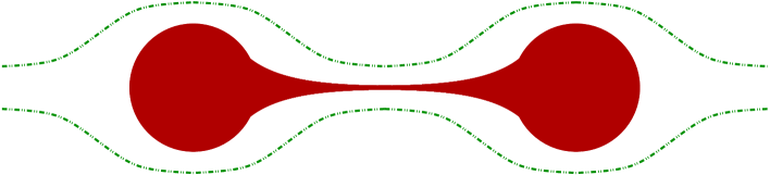
Figure 4: The sets $E$ and $G_{\eta_{0}}$ in the proof of Theorem 1.3.

3.2 Completion of the proof of Theorem 1.3

With Lemma 3.1, we can complete the proof of Theorem 1.3. For this, we take $t_{r}>0$ to be the extinction time of the ball $B_{r/10^{6}}$. We define

$$\eta_{0}:=\min\left\{\frac{t_{r}}{8r},\,\frac{r}{128\pi^{2}}\right\}\quad{\mbox{ and }}\quad\eta(t):=\eta_{0}-\frac{t}{4r}.$$

We take $q_{\pm}:=\left(\pm\frac{1}{2},0\right)$ and

$$N:=[-q_{-},q_{+}]\times\left[-\frac{\eta_{0}}{2},\frac{\eta_{0}}{2}\right].$$

We consider a connected and smooth set $E\subset(-1,1)\times\left(-\frac{r}{2},\frac{r}{2}\right)$ such that

$$G_{\eta_{0}}\supseteq E\supseteq B_{r/10^{6}}(q_{-})\cup B_{r/10^{6}}(q_{+})\cup N,$$

with $E\cap\{|x|\leqslant 1/10\}=N$, see Figure 4. Confronting with halfplanes, the comparison principle for (1.2) (see e.g. Section 3.3 in [MR3023439]) gives that also the evolution $E_{t}$ lies in $(-1,1)\times\left(-\frac{r}{2},\frac{r}{2}\right)$. In addition, the velocity of $G_{\eta(t)}$ in modulus coincides with $\frac{1}{4r}$, which is less than the $r$-curvature of $G_{\eta(t)}$, thanks to (3.1). As a consequence of this and of the comparison principle, we obtain that $E_{t}\subseteq G_{\eta(t)}$. Since $t_{\star}:=4r\eta_{0}<t_{r}$ and $\eta(t_{\star})=0$, we have that $G_{\eta(t_{\star})}$ develops a neck singularity, and so does $E_{t}$ for some $t\in(0,t_{\star})$. This completes the proof of Theorem 1.3.

4 Proof of Theorem 1.4

4.1 Geometric barriers

This section is devoted to the construction of an explicit barrier for the geometric flow in (1.2). Roughly speaking, this barrier is constructed by taking the region trapped between a graph and its reflection along the horizontal axis. Such graph is constructed by interpolating a parabola with curvature comparable to $r$ near the origin with a uniformly concave function. The interpolation will occur when the values on the abscissa are of order $r$ and the functions are also of order $r$, but the gradients are of order $1$. This quantitative construction is needed to compute efficiently the $r$-curvatures in (1.1) and the example that we provide may turn out to be useful also in other cases.

We fix $M\geqslant 1$, to be taken appropriately large in the sequel. We also consider a bump function $\varphi\in C^{\infty}_{0}([-2,2],\,[0,1])$, with $\varphi=1$ in $[-1,1]$, $|\varphi^{\prime}|\leqslant 2$ and $|\varphi^{\prime\prime}|\leqslant 2$. We also define $\rho:=Mr$ and, for any $x\in\mathbb{R}$,

$$g(x):=\frac{x^{2}}{2M^{2}\rho}\,\varphi\left(\frac{x}{\rho}\right)+\left(1-\varphi\left(\frac{x}{\rho}\right)\right)\,\frac{|x|}{M^{2}\,(1+|x|)}.$$

For any $\varepsilon>0$ we set $g_{\varepsilon}(x):=\varepsilon+g(x)$ and

$$F_{\varepsilon}:=\Big{\{}(x,y)\in\mathbb{R}^{2}{\mbox{ s.t. }}|y|\leqslant g_{\varepsilon}(x)\Big{\}}.$$

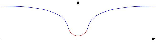
Figure 5: The function $g_{\varepsilon}$.

The graph of $g_{\varepsilon}$ is depicted in Figure 5. The set $F_{\varepsilon}$ is a useful barrier for the $r$-geometric flow, according to the following calculation:

Lemma 4.1.

There exist $M>1$ and $c_{0}\in(0,1)$ such that if $r\in\left(0,\frac{1}{M}\right)$ and $\varepsilon\in\left(0,\frac{r}{M}\right)$ then

$$\kappa_{r}(F_{\varepsilon},p)\geqslant c_{0}\qquad{\mbox{for any }}p=(p_{1},p_{2})\in\partial F_{\varepsilon}{\mbox{ with }}|p_{1}|\leqslant 10.$$ (4.1)

Proof.

By symmetry, we can reduce our analysis to the first quadrant, i.e. prove (4.1) for $p=(p_{1},p_{2})\in\partial F_{\varepsilon}$, with $p_{1}\in[0,10]$ and $p_{2}\in[0,+\infty)$. For any $x\in[0,10]$, it holds that

$$g^{\prime}_{\varepsilon}(x) = \frac{x}{M^{2}\rho}\,\varphi\left(\frac{x}{\rho}\right)+\frac{x^{2}}{2M^{2}\rho^{2}}\,\varphi^{\prime}\left(\frac{x}{\rho}\right)$$

$$\qquad-\varphi^{\prime}\left(\frac{x}{\rho}\right)\,\frac{x}{M^{2}\,\rho\,(1+x)}+\left(1-\varphi\left(\frac{x}{\rho}\right)\right)\,\frac{1}{M^{2}\,(1+x)^{2}}$$

and

$$g^{\prime\prime}_{\varepsilon}(x) = \frac{1}{M^{2}\rho}\,\varphi\left(\frac{x}{\rho}\right)+\frac{2x}{M^{2}\rho^{2}}\,\varphi^{\prime}\left(\frac{x}{\rho}\right)+\frac{x^{2}}{2M^{2}\rho^{3}}\,\varphi^{\prime\prime}\left(\frac{x}{\rho}\right)$$

$$\qquad-\varphi^{\prime\prime}\left(\frac{x}{\rho}\right)\,\frac{x}{M^{2}\,\rho^{2}\,(1+x)}-\varphi^{\prime}\left(\frac{x}{\rho}\right)\,\frac{2}{M^{2}\,\rho\,(1+x)^{2}}$$

$$\qquad-\left(1-\varphi\left(\frac{x}{\rho}\right)\right)\,\frac{2}{M^{2}\,(1+x)^{3}}.$$

Consequently, for any $x\in[0,10]$,

$$\begin{split}|g^{\prime\prime}_{\varepsilon}(x)|\,&\leqslant\frac{1}{M^{2}\rho}+\frac{8\rho}{M^{2}\rho^{2}}+\frac{8\rho^{2}}{2M^{2}\rho^{3}}+\frac{4\rho}{M^{2}\,\rho^{2}}+\frac{4}{M^{2}\,\rho}+\frac{2}{M^{2}}\\ &=\frac{(21+2\rho)}{M^{2}\,\rho}\\ &=\frac{(21+2Mr)}{M^{3}\,r}\\ &\leqslant\frac{23}{M^{3}\,r}.\end{split}$$ (4.2)

Also,

$${\mbox{for any }}x\in[2\rho,10],\qquad|g^{\prime}_{\varepsilon}(x)|=\frac{1}{M^{2}\,(1+x)^{2}}\leqslant\frac{1}{M^{2}}.$$ (4.3)

Moreover,

$${\mbox{for any }}x\in[2\rho,10],\qquad g^{\prime\prime}_{\varepsilon}(x)=-\frac{2}{M^{2}\,(1+x)^{3}}\in\left[-\frac{2}{M^{2}},-\frac{2}{M^{2}\,11^{3}}\right].$$ (4.4)

On the other hand,

$$\begin{split}{\mbox{for any }}x\in[0,2\rho],\qquad g_{\varepsilon}(x)\,&\leqslant\varepsilon+\frac{4\rho^{2}}{2M^{2}\rho}+\frac{2\rho}{M^{2}}\\ &=\varepsilon+\frac{4\rho}{M^{2}}\\ &\leqslant\frac{5r}{M}.\end{split}$$ (4.5)

In the same way, we see that

$$\begin{split}{\mbox{for any }}x\in[0,2\rho],\qquad|g^{\prime}_{\varepsilon}(x)|\,&\leqslant\frac{2\rho}{M^{2}\rho}+\frac{8\rho^{2}}{2M^{2}\rho^{2}}+\frac{4\rho}{M^{2}\,\rho}+\frac{1}{M^{2}}\\ &\leqslant\frac{11}{M^{2}}.\end{split}$$ (4.6)

Now, since the curvature of the graph is given by

$$-\left(\frac{g_{\varepsilon}^{\prime}}{\sqrt{1+(g_{\varepsilon}^{\prime})^{2}}}\right)^{\prime}=-\frac{g_{\varepsilon}^{\prime\prime}}{(1+(g_{\varepsilon}^{\prime})^{2})^{3/2}},$$

it follows from (4.2) that

$${\mbox{the curvature of the graph is bounded everywhere in absolute value by }}\frac{23}{M^{3}\,r},$$ (4.7)

which is less than $\frac{1}{r}$ if $M$ is sufficiently large. Hence, the set $F_{\varepsilon}$ can always be touched from outside by balls of radius $r$, i.e. $B_{r,p}^{\mathrm{ext}}\subseteq\mathbb{R}^{2}\setminus F_{\varepsilon}$ and so, by (1.1),

$$\kappa_{r}^{+}(F_{\varepsilon},p)=\frac{\kappa(F_{\varepsilon},p)}{2}+\frac{1}{2r}.$$ (4.8)

Similarly, from (4.3) and (4.4), we infer that

$$\begin{split}&{\mbox{the curvature of the graph with abscissa in $[2\rho,10]$}}\\ &{\mbox{is bounded from below by }}\frac{1}{M^{2}\,11^{3}}.\end{split}$$ (4.9)

Now, to compute $\kappa_{r}^{-}(F_{\varepsilon},p)$ we distinguish the two cases $p_{1}\in[0,2\rho]$ and $p_{1}\in[2\rho,10]$. If $p_{1}\in[0,2\rho]$ we claim that

$$B_{r,p}^{\mathrm{int}}\cap\{y<-g_{\varepsilon}(x)\}\neq\emptyset.$$ (4.10)

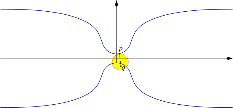
Figure 6: The geometry involved in the proof of (4.10).

To check this, we use Figure 6 and we notice that the exterior normal at $p$ is given by

$$\nu_{F_{\varepsilon}}(p)=\frac{(-g_{\varepsilon}^{\prime}(p_{1}),1)}{\sqrt{1+(g_{\varepsilon}^{\prime}(p_{1}))^{2}}}$$

and

$$q=(q_{1},q_{2}):=p-r\nu_{F_{\varepsilon}}(p)-\frac{r\nu_{F_{\varepsilon}}(p)}{2}\in B_{r,p}^{\mathrm{int}}.$$

So, to prove (4.10), it is enough to check that

$$q_{2}<-g_{\varepsilon}(q_{1}).$$ (4.11)

As a matter of fact, since $p_{2}=g_{\varepsilon}(p_{1})$,

$$q_{2}+g_{\varepsilon}(q_{1}) = \left(p-\frac{3r\nu_{F_{\varepsilon}}(p)}{2}\right)_{2}+g_{\varepsilon}\left(\left(p-\frac{3r\nu_{F_{\varepsilon}}(p)}{2}\right)_{1}\right)$$

$$= g_{\varepsilon}(p_{1})-\frac{3r}{2\sqrt{1+(g_{\varepsilon}^{\prime}(p_{1}))^{2}}}+g_{\varepsilon}\left(p_{1}+\frac{3r\,g_{\varepsilon}^{\prime}(p_{1})}{2\sqrt{1+(g_{\varepsilon}^{\prime}(p_{1}))^{2}}}\right)$$

by (4.6) $$\leqslant 2g_{\varepsilon}(p_{1})-\frac{3r}{2\sqrt{1+(11/M^{2})^{2}}}+\sup_{x\in[0,10]}|g^{\prime}_{\varepsilon}(x)|\,\frac{3r\,|g_{\varepsilon}^{\prime}(p_{1})|}{2\sqrt{1+(g_{\varepsilon}^{\prime}(p_{1}))^{2}}}$$

by (4.3), (4.5) and (4.6) $$\leqslant \frac{10\,r}{M}-\frac{3r}{2\sqrt{1+(11/M^{2})^{2}}}+\left(\frac{11}{M^{2}}\right)^{2}\,\frac{3r}{2}$$

$$\leqslant \frac{r}{2}-r,$$

as long as $M$ is sufficiently large. This proves (4.11), and so (4.10).

Then, from (1.1) and (4.10), we obtain that

if $$p_{2}\in[0,2\rho] \kappa^{-}_{r}(F_{\varepsilon},p)=0$$, then .

From this and (4.8), we conclude that

$${\mbox{if $p_{2}\in[0,2\rho]$, then }}\kappa_{r}(F_{\varepsilon},p)=\frac{\kappa(F_{\varepsilon},p)}{2}+\frac{1}{2r}.$$

This and (4.7) imply that

$${\mbox{if $p_{2}\in[0,2\rho]$, then }}\kappa_{r}(F_{\varepsilon},p)\geqslant-\frac{23}{2\,M^{3}\,r}+\frac{1}{2r}\geqslant\frac{1}{3r},$$ (4.12)

as long as $M$ is large enough.

On the other hand, by (4.9), we know that

$${\mbox{if $p_{2}\in[2\rho,10]$, then }}\kappa(F_{\varepsilon},p)\geqslant\frac{1}{M^{2}\,11^{3}}$$

and therefore, recalling (1.1) and (4.8), we have that

$${\mbox{if $p_{2}\in[2\rho,10]$, then }}\kappa_{r}(F_{\varepsilon},p) = \kappa_{r}^{+}(F_{\varepsilon},p)+\kappa_{r}^{-}(F_{\varepsilon},p)$$

$$\geqslant \frac{\kappa(F_{\varepsilon},p)}{2}+\frac{1}{2r}+\min\left\{0,\;\frac{\kappa(F_{\varepsilon},p)}{2}-\frac{1}{2r}\right\}$$

$$= \min\left\{\frac{\kappa(F_{\varepsilon},p)}{2}+\frac{1}{2r},\;\kappa(F_{\varepsilon},p)\right\}$$

$$\geqslant \frac{1}{2\,M^{2}\,11^{3}}.$$

The desired result now follows plainly from this inequality and (4.12). ∎

4.2 Completion of the proof of Theorem 1.4

With the construction in Lemma 4.1, the proof of Theorem 1.4 follows by a comparison principle, with an argument similar to that in Section 3.2. We give the full argument for the facility of the reader. We take $M$ and $c_{0}$ as in Lemma 4.1 and we define, for any $t\geqslant 0$,

$$\varepsilon(t):=\frac{r}{2M}-\frac{c_{0}\,t}{2}.$$

The set $F_{\varepsilon(t)}$ falls under the assumption of Lemma 4.1, so, by (4.1),

$$\kappa_{r}(F_{\varepsilon(t)},p)\geqslant c_{0}\qquad{\mbox{for any }}p=(p_{1},p_{2})\in\partial F_{\varepsilon(t)}{\mbox{ with }}|p_{1}|\leqslant 10.$$ (4.13)

Moreover, using balls of radius $r/2$ centered at points $p=(p_{1},0)$ with $|p_{1}|$ large, we see that the portion of the barrier $F_{\varepsilon(t)}$ coming from infinity does not collapse instantaneously.

Now we set $q_{\pm}:=(\pm 3,0)$ and

$$N:=[-3,3]\times\left[-\frac{\varepsilon(0)}{2},\frac{\varepsilon(0)}{2}\right],$$

and we take $R>0$ and a connected and smooth set $E\subset F_{\varepsilon(0)}$ such that

$$E\supseteq B_{R}(q_{-})\cup B_{R}(q_{+})\cup N.$$

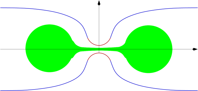
Figure 7: The sets $E$ and $F_{\varepsilon(0)}$.

The geometric situation of this proof is depicted in Figure 7. Notice that we can take such $R$ independent of $r$ and the modulus of the velocity of $F_{\varepsilon(t)}$ is $\frac{c_{0}}{2}$, which is less than the normal velocity of the flow (1.2), thanks to (4.13). Therefore, by comparison principle (see e.g. Section 3.3 in [MR3023439]), we conclude that $E_{t}\subset\{|x|\leqslant 10\}$ and, more importantly, $E_{t}\subset F_{\varepsilon(t)}$ for all $t\in[0,T)$, being $T$ the extinction time. Since the extinction time $T$ is bounded from below by the one of the ball $B_{R}$, which is independent of $r$, we can take $r$ sufficiently small and suppose that $\frac{r}{c_{0}\,M}<T$. But, since $F_{\varepsilon(t)}$ develops a neckpinch at time $t=\frac{r}{c_{0}\,M}$, also any viscosity evolution of the set $E_{t}$ develops a singularity before this time, and gets disconnected. This completes the proof of Theorem 1.4.

5 Proof of Theorem 1.5

We compute the evolution of the curvature of a geometric flow with normal velocity $v$, assuming that such evolution is $C^{1}$ in time and $C^{2}$ in space. For this, we denote by $s$ the arclength variable and we recall (see e.g. formula (9) in [MR2863468]) that if a set $F_{t}$ is a solution of $\partial_{t}x_{t}\cdot\nu_{F_{t}}(x_{t})=-v(x_{t})$ then

$$\partial_{t}\kappa(F_{t},x_{t})=\partial_{ss}^{2}v(x_{t})+\kappa^{2}(F_{t},x_{t})\,v(x_{t}).$$ (5.1)

Furthermore, comparing with halfplanes, we see that the evolution of $E_{t}$ is $r$-thin for any time $t$ (till extinction). Therefore, $E_{t}$ does not contain balls of radius $r$ and then, in view of (1.1), it holds that

$$\kappa_{r}^{-}(E_{t},x_{t})=0\quad{\mbox{ for any }}x_{t}\in\partial E_{t}.$$ (5.2)

Now, suppose that $E_{t}$ is convex: it follows from (1.1) that

$$\kappa_{r}^{+}(E_{t},x_{t})=\frac{\kappa(E_{t},x_{t})}{2}+\frac{1}{2r}.$$

This and (5.2) give that

$$\kappa_{r}(E_{t},x_{t})=\frac{\kappa(E_{t},x_{t})}{2}+\frac{1}{2r}.$$

As a consequence,

$$\kappa_{r}(E_{t},x_{t})\geqslant\frac{1}{2r}$$

and $$\partial^{2}_{ss}\kappa_{r}(E_{t},x_{t})=\frac{\partial^{2}_{ss}\kappa(E_{t},x_{t})}{2}.$$

In particular, by (5.1), we have that, if $E_{t}$ is a solution of the geometric flow in (1.2), till it is convex it holds that

$$\begin{split}\partial_{t}\kappa(E_{t},x_{t})\,&=\partial_{ss}^{2}\kappa_{r}(E_{t},x_{t})+\kappa^{2}(E_{t},x_{t})\,\kappa_{r}(E_{t},x_{t})\\ &=\frac{\partial^{2}_{ss}\kappa(E_{t},x_{t})}{2}+\kappa^{2}(E_{t},x_{t})\,\kappa_{r}(E_{t},x_{t}).\end{split}$$

Hence, if $x_{t}^{\star}$ is minimal for $\kappa(E_{t},\cdot)$, we have that

$$\partial^{2}_{ss}\kappa(E_{t},x_{t}^{\star})\geqslant 0$$

and

$$\partial_{t}\kappa(E_{t},x_{t})\geqslant\kappa^{2}(E_{t},x_{t})\kappa_{r}(E_{t},x_{t})\geqslant 0.$$

This gives that $\kappa(E_{t},\cdot)$ is nondecreasing at the minimal points, and thus nonnegative, which completes the proof of Theorem 1.5.

6 Proof of Theorem 1.6

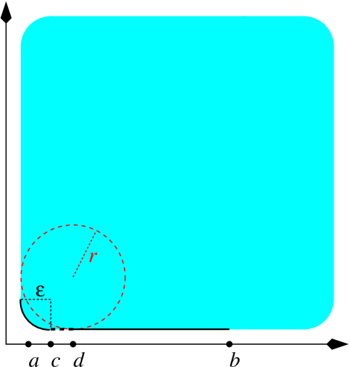
Figure 8: The set in the proof of Theorem 1.6.

We construct a convex set $E$ as depicted in Figure 8. Namely, we consider the smoothing of a square of side $1>>r$ in which the corners are rounded by a curve with curvature of order $\varepsilon<<r$. Notice that the curvature of $\partial E$ vanishes along the dashed and solid line on the bottom of Figure 8, and it is of the order of $1/\varepsilon$ along the solid arc. As for the $r$-curvature, from (1.1) we see that $\kappa_{r}$ is equal to $\kappa$ along the solid line and to $\frac{\kappa}{2}+\frac{1}{2r}$ along the dashed line and the solid arc. That is, $\kappa_{r}$ is equal to $0$ along the solid line, equal to $\frac{1}{2r}$ along the dashed line and of order $\frac{1}{\varepsilon}$ along the solid arc.

Consequently, if we put Cartesian axes as in Figure 8, we can describe $\kappa_{r}$ along the bottom of the set $E$ by a function $\varphi$, and, considering intervals $(a,b)\supset(c,d)$ as in Figure 8, it holds that $\varphi=\frac{1}{2r}$ on $(c,d)$ and $\varphi=0$ on $(d,b)$. In particular,

$$\varphi$$ is not convex. (6.1)

Now, to establish Theorem 1.6 we argue by contradiction and suppose that the set $E$ evolves in time $t\in[0,T)$ into a convex set $E_{t}$. We point out that the set

$$\partial E_{t}\cap\big{(}\mathbb{R}\times(-h,h)\big{)} t\in[0,T)$$ is a graph in the vertical direction for all , (6.2)

provided that $h$, $T>0$ are chosen appropriately small. Indeed, if not, a vertical segment would meet $\partial E_{t}\cap\big{(}\mathbb{R}\times(-h,h)\big{)}$ at least twice; then, since another intersection with $\partial E_{t}$ must occur close to the top, this would contradict the convexity of $E_{t}$.

Hence, as a consequence of (6.2), the boundary of the set $E_{t}$ can be locally described, in the vicinity of the interval $(a,b)$ by a convex function $\Psi=\Psi(x,t)$. By (1.2) and the fact that

$$\Psi(x,0) x\in(c,b)$$ is constant for all , (6.3)

we know that the velocity of the flow at time $0$ coincides with $\partial_{t}\Psi(x,0)$, hence

$$\partial_{t}\Psi(x,0)=\varphi(x)\quad{\mbox{ for all~{}$x\in(c,b)$}}.$$ (6.4)

Also, since $\Psi$ is convex, for any $x$, $y\in(c,b)$, any $\vartheta\in[0,1]$ and any $t\in(0,T)$ we have that

$$\Psi\big{(}(1-\vartheta)x+\vartheta y,t\big{)}\leqslant(1-\vartheta)\Psi(x,t)+\vartheta\Psi(y,t),$$

and therefore, in view of (6.3) and (6.4),

$$\varphi((1-\vartheta)x+\vartheta y) = \partial_{t}\Psi\big{(}(1-\vartheta)x+\vartheta y,0\big{)}$$

$$= \lim_{t\searrow 0}\frac{\Psi\big{(}(1-\vartheta)x+\vartheta y,t\big{)}-\Psi\big{(}(1-\vartheta)x+\vartheta y,0\big{)}}{t}$$

$$\leqslant \lim_{t\searrow 0}\frac{(1-\vartheta)\Psi(x,t)+\vartheta\Psi(y,t)}{t}-\frac{\Psi\big{(}(1-\vartheta)x+\vartheta y,0\big{)}}{t}$$

$$= \lim_{t\searrow 0}\frac{(1-\vartheta)\Psi(x,t)+\vartheta\Psi(y,t)}{t}-\frac{(1-\vartheta)\Psi\big{(}x,0\big{)}+\vartheta\Psi\big{(}y,0\big{)}}{t}$$

$$= \lim_{t\searrow 0}\frac{(1-\vartheta)\big{(}\Psi(x,t)-\Psi(x,0)\big{)}+\vartheta\big{(}\Psi(y,t)-\Psi(y,0)\big{)}}{t}$$

$$= (1-\vartheta)\partial_{t}\Psi(x,0)+\vartheta\partial_{t}\Psi(y,0)$$

$$= (1-\vartheta)\varphi(x)+\vartheta\varphi(y).$$

This gives that $\varphi$ is convex in $(c,b)$, which is a contradiction with (6.1) and so Theorem 1.6 is proved.

7 Proof of Theorem 1.7

Without loss of generality, we can normalize the speed $c$ to be equal to $1$. Such dilation, in the new coordinate frame, transforms the condition $c\in(0,r)$ into

$$r>1.$$ (7.1)

Then, if $h$ is a traveling wave as in (1.3) with $c=1$ for a geometric flow with inner normal velocity $v$, one sees that $h$ is a solution of

$$v(x)\,\sqrt{1+|h^{\prime}(x)|^{2}}=1.$$ (7.2)

In particular, for the classical mean curvature flow, we have that

$$v(x)=\frac{h^{\prime\prime}(x)}{(1+|h^{\prime}(x)|^{2})^{3/2}},$$

and so (7.2) becomes

$$\frac{h^{\prime\prime}(x)}{1+|h^{\prime}(x)|^{2}}=1.$$ (7.3)

Similarly, in the regime in which $\kappa_{r}=\frac{\kappa}{2}+\frac{1}{2r}$, the flow in (1.2) and (7.2) yield the equation

$$\frac{h^{\prime\prime}(x)}{1+|h^{\prime}(x)|^{2}}=2-\frac{\sqrt{1+|h^{\prime}(x)|^{2}}}{r}.$$ (7.4)

Our objective is now to consider a (suitable translation of a) solution $h_{\infty}$ of (7.3) (far from the origin) and glue it to a solution $h_{0}$ of (7.4) (near the origin). The joint will be done in such a way that the final curve is $C^{1,1}$ (roughly speaking, the building arcs will share the tangent line at the matching point).

To implement this construction, we consider the Cauchy problem

$$\left\{\begin{matrix}\phi^{\prime}(x)=2(1+|\phi(x)|^{2})-\displaystyle\frac{1}{r}\,(1+|\phi(x)|^{2})^{3/2},\\ \phi(0)=0.\end{matrix}\right.$$ (7.5)

The solution to this problem exists (and it is unique) for small values of $x$, and we extend it to its largest existence interval $(x_{-},x_{+})$, with $-\infty\leqslant x_{-}<0<x_{+}\leqslant+\infty$. We claim that

$${\mbox{for all~{}$x\in(x_{-},x_{+})$, we have that~{}$\phi(x)\leqslant\sqrt{4r^{2}-1}$}}.$$ (7.6)

Indeed, suppose, by contradiction, that there exists $\bar{x}\in(x_{-},x_{+})$ such that $\phi(\bar{x})>\sqrt{4r^{2}-1}$. Then, for any $\varepsilon>0$ sufficiently small, there exists ${\bar{x}_{\varepsilon}}$ on the segment joining $0$ to $\bar{x}$ such that $\phi({\bar{x}_{\varepsilon}})=\sqrt{4r^{2}(1+\varepsilon)-1}$ with $\phi^{\prime}({\bar{x}_{\varepsilon}})\geqslant 0$. Then, we have that

$$0 \leqslant \phi^{\prime}({\bar{x}_{\varepsilon}})$$

$$= 2(1+|\phi({\bar{x}_{\varepsilon}})|^{2})-\frac{1}{r}\,(1+|\phi({\bar{x}_{\varepsilon}})|^{2})^{3/2}$$

$$= 2(4r^{2}(1+\varepsilon))-\frac{1}{r}\,(4r^{2}(1+\varepsilon))^{3/2}$$

$$= 8r^{2}(1+\varepsilon)-8r^{2}(1+\varepsilon)^{3/2}$$

$$= 8r^{2}(1+\varepsilon)(1-\sqrt{1+\varepsilon})$$

$$< 0,$$

which is a contradiction, proving (7.6).

We also have that

$${\mbox{for all~{}$x\in(x_{-},x_{+})$, it holds that~{}$\phi(x)\geqslant 0$}}.$$ (7.7)

Indeed, suppose, by contradiction, that for any $\varepsilon>0$ small enough there exists $\tilde{x}_{\varepsilon}\in(x_{-},x_{+})$ such that $\phi({\tilde{x}_{\varepsilon}})=-\varepsilon$ with $\phi^{\prime}({\tilde{x}_{\varepsilon}})\leqslant 0$. Then, it holds that

$$0 \geqslant \phi^{\prime}({\tilde{x}_{\varepsilon}})$$

$$= 2(1+|\phi({\tilde{x}_{\varepsilon}})|^{2})-\frac{1}{r}\,(1+|\phi({\tilde{x}_{\varepsilon}})|^{2})^{3/2}$$

$$= 2(1+\varepsilon^{2})-\frac{1}{r}\,(1+\varepsilon^{2})^{3/2}.$$

Hence, taking $\varepsilon$ arbitrarily small, we obtain that $0\geqslant 2-\frac{1}{r}$, which gives a contradiction with (7.1), thus proving (7.7).

As a consequence of (7.6) and (7.7), we obtain that $x_{+}=+\infty$ and $x_{-}=-\infty$, and so $\phi$ is a global solution of (7.5). In addition, since $x\mapsto-\phi(-x)$ is also a solution of (7.5), by the uniqueness result of the Cauchy problem we obtain that $\phi(x)=-\phi(-x)$, i.e.

$$\phi$$ is odd. (7.8)

Moreover, from (7.6), we have that

$$2-\frac{1}{r}\sqrt{1+|\phi(x)|^{2}}\geqslant 0$$

and so, by (7.5),

$$\phi^{\prime}(x)=(1+|\phi(x)|^{2})\left(2-\displaystyle\frac{1}{r}\sqrt{1+|\phi(x)|^{2}}\right)\geqslant 0.$$

Accordingly,

$$\phi$$ is monotone nondecreasing (7.9)

and so the following limit exists

$$\ell:=\lim_{x\to+\infty}\phi(x).$$

Also, by (7.5), (7.6) and (7.9), it holds that

$$0=\lim_{x\to+\infty}\phi^{\prime}(x)=2(1+\ell^{2})-\frac{1}{r}\,(1+\ell^{2})^{3/2},$$

and therefore

$$\lim_{x\to+\infty}\phi(x)=\ell=\sqrt{4r^{2}-1}.$$

We also define

$$h_{0}(x):=\int_{0}^{x}\phi(\xi)\,d\xi.$$ (7.10)

Notice that $h_{0}$ is convex, in view of the monotonicity of $\phi$, and it is even, due to (7.8). Also, by (7.5), we know that

$$\left\{\begin{matrix}h_{0}^{\prime\prime}(x)=2(1+|h_{0}^{\prime}(x)|^{2})-\displaystyle\frac{1}{r}\,(1+|h_{0}^{\prime}(x)|^{2})^{3/2},\\ h_{0}(0)=0=h_{0}^{\prime}(0),\end{matrix}\right.$$

and so $h_{0}$ is a solution of (7.4).

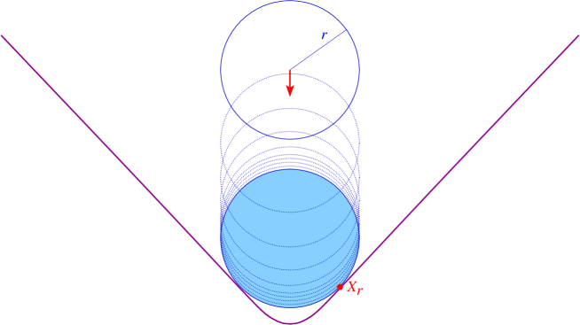
Figure 9: Dropping balls inside the supergraph of $h_{0}$.

The idea is now to use a “dropping the ball in the basket” method, see Figure 9. Namely, we slide a ball $B_{r}(te_{n})$ from $t=+\infty$ downwards, till it touches the graph of $h_{0}$. We denote by $X_{r}=(x_{r},h_{0}(x_{r}))$ a touching point situated on the right branch of the graph of $h_{0}$. We also denote the curvature of the supergraph of $h_{0}$ at a point $X=(x,h_{0}(x))$ by $\kappa_{0}(x)$. Since the supergraph of $h_{0}$ contains a ball of radius $r$ tangent at $x_{r}$, we have that

$$\kappa_{0}(x_{r})\leqslant\frac{1}{r}.$$ (7.11)

On the other hand, by (7.4),

$$\kappa_{0}(x)=\frac{h^{\prime\prime}_{0}(x)}{(1+|h^{\prime}_{0}(x)|^{2})^{3/2}}=\frac{1}{\sqrt{1+|h^{\prime}_{0}(x)|^{2}}}\left(2-\frac{\sqrt{1+|h^{\prime}_{0}(x)|^{2}}}{r}\right)=\frac{2}{\sqrt{1+|h^{\prime}_{0}(x)|^{2}}}-\frac{1}{r}.$$ (7.12)

By (7.11) and (7.12), it follows that

$$\frac{1}{r}\geqslant\kappa_{0}(x_{r})=\frac{2}{\sqrt{1+|h^{\prime}_{0}(x_{r})|^{2}}}-\frac{1}{r}$$

and therefore

$$h_{0}^{\prime}(x_{r})\geqslant\sqrt{r^{2}-1}.$$ (7.13)

Now we consider the “standard grim reaper”

$$\left[-\frac{\pi}{2},\frac{\pi}{2}\right]\ni x\mapsto h_{\infty}(x)=-\log(\cos x),$$ (7.14)

and we define

$$\tilde{x}_{r}:=\arctan h_{0}^{\prime}(x_{r}).$$ (7.15)

Notice that, in view of (7.1), we have that $\tilde{x}_{r}\in\left(0,\frac{\pi}{2}\right)$. We also set

$$h_{\star}(x):=\left\{\begin{matrix}h_{0}(x)&{\mbox{ if }}|x|\leqslant x_{r},\\ h_{\infty}(x+\tilde{x}_{r}-x_{r})-h_{\infty}(\tilde{x}_{r})+h_{0}(x_{r})&{\mbox{ if }}x\in\left(x_{r},\,\displaystyle\frac{\pi}{2}+x_{r}-\tilde{x}_{r}\right),\\ h_{\infty}(x-\tilde{x}_{r}+x_{r})-h_{\infty}(\tilde{x}_{r})+h_{0}(x_{r})&{\mbox{ if }}x\in\left(-\displaystyle\frac{\pi}{2}+\tilde{x}_{r}-x_{r},\,-x_{r}\right).\end{matrix}\right.$$ (7.16)

The function $h_{\star}$ is depicted in Figure 10. By inspection, we see that $h_{\star}$ is continuous and even. Also, by (7.14) and (7.15), we have that

$$h_{\infty}^{\prime}(\tilde{x}_{r})=\tan\tilde{x}_{r}=h_{0}^{\prime}(x_{r}),$$

and so $h_{\star}\in C^{1,1}(\mathbb{R})$.

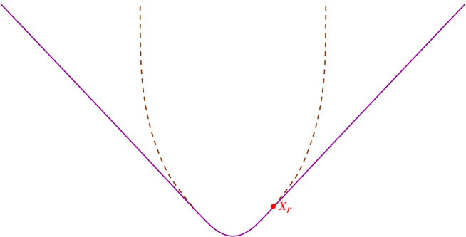
Figure 10: The new traveling wave in (7.16). The dashed curves are branches of classical grim reapers. The solid curve represents the graph of $h_{0}$.

It is also useful to observe that

the touching point $$X_{r} h_{0}$$ on the right branch of  is unique. (7.17)

Indeed, from (7.12) and the monotonicity of $h_{0}^{\prime}=\phi$ it follows that $\kappa_{0}(x)\leqslant\kappa_{0}(x_{r})$ for any $x>x_{r}$. This and (7.11) yield that $\kappa_{0}(x)\leqslant 1/r$ for any $x>x_{r}$, from which it follows that there cannot be another touching point on the right branch of $h_{0}$ with $x>x_{r}$. On the other hand, if there was another touching point $\tilde{X}_{r}$ with $\tilde{x}_{r}<x_{r}$, then this observation would also imply that there cannot be a touching point on the right branch of $h_{0}$ with $x>\tilde{x}_{r}$, which gives a contradiction and completes the proof of (7.17).

We observe that, by (7.1) and (7.12),

$$\kappa_{0}(0)=\frac{2}{\sqrt{1+|h^{\prime}_{0}(0)|^{2}}}-\frac{1}{r}=2-\frac{1}{r}>1>\frac{1}{r}$$

and this implies that the touching point cannot occur at the origin, namely $x_{r}>0$.

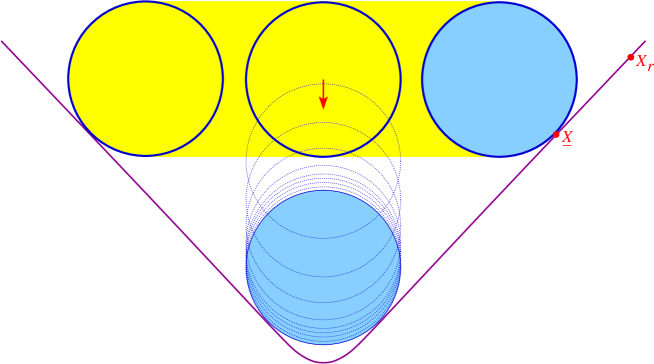
Figure 11: Proof of (7.18).

Furthermore,

$$\begin{split}&{\mbox{the graph of~{}$h_{0}$ cannot be touched from above}}\\ &{\mbox{by a ball of radius~{}$r$ at any point~{}$X=(x,h_{0}(x))$ with~{}$|x|<x_{r}$.}}\end{split}$$ (7.18)

Indeed, suppose by contradiction that the graph of $h_{0}$ is touched from above by $B_{r}(\underline{p}_{1},\underline{p}_{2})$ at a point $\underline{X}=(\underline{x},h_{0}(\underline{x}))$ with $0<\underline{x}<x_{r}$. Since $h_{0}$ is even, it follows that $B_{r}(-\underline{p}_{1},\underline{p}_{2})$ is also contained in the supergraph of $h_{0}$. Hence, by convexity, the ball $B_{r}(0,\underline{p}_{2})$ is contained in the supergraph of $h_{0}$. Dropping down such ball, we obtain a touching point $\hat{X}=(\hat{x},h_{0}(\hat{x}))$ with $0<\hat{x}<x_{r}$, thus producing a contradiction with (7.17) and completing the proof of (7.18) (see Figure 11 for a sketch of this argument).

To complete the proof of Theorem 1.7, we now check that the translating supergraph of $h_{\star}$ is a solution of the geometric flow in (1.2). For this, since this supergraph is convex, and $h_{\infty}$ and $h_{0}$ are solutions of (7.3) and (7.4), respectively, recalling (7.18) it is enough to check that

$$\begin{split}&{\mbox{the curvature of the supergraph is smaller than~{}$\displaystyle\frac{1}{r}$ when~{}$|x|\in\left(x_{r},\,\displaystyle\frac{\pi}{2}+x_{r}-\tilde{x}_{r}\right)$.}}\end{split}$$ (7.19)

To this aim, we observe that when $x\in\left(x_{r},\,\frac{\pi}{2}+x_{r}-\tilde{x}_{r}\right)$ we have that $x+\tilde{x}_{r}-x_{r}\in\left(\tilde{x}_{r},\,\frac{\pi}{2}\right)\subseteq\left(0,\,\frac{\pi}{2}\right)$, and thus we deduce from (7.13), (7.14) and (7.15) that

$$\frac{h_{\star}^{\prime\prime}(x)}{(1+|h_{\star}^{\prime}(x)|^{2})^{3/2}}=\frac{h_{\infty}^{\prime\prime}(x+\tilde{x}_{r}-x_{r})}{(1+|h_{\infty}^{\prime}(x+\tilde{x}_{r}-x_{r})|^{2})^{3/2}}=|\cos(x+\tilde{x}_{r}-x_{r})|$$

$$\qquad=\cos(x+\tilde{x}_{r}-x_{r})\leqslant\cos(\tilde{x}_{r})=\cos(\arctan h_{0}^{\prime}(x_{r}))\leqslant\cos(\arctan\sqrt{r^{2}-1})=\frac{1}{r}.$$

This establishes (7.19) when $x\in\left(x_{r},\,\frac{\pi}{2}+x_{r}-\tilde{x}_{r}\right)$, and the case $x\in\left(-\frac{\pi}{2}+\tilde{x}_{r}-x_{r},\,-x_{r}\right)$ is symmetric. Hence, the proof of (7.19), and so of Theorem 1.7, is complete.

Remark 7.1.

We observe that the translating solution constructed in Theorem 1.7 is only $C^{1,1}$ and not $C^{2}$ in principle. On the other hand, such regularity is enough to define the velocity field at any point in a continuous way, thanks to (7.2).

Addresses:

Serena Dipierro & Enrico Valdinoci. Department of Mathematics and Statistics, University of Western Australia, 35 Stirling Hwy, Crawley WA 6009, Australia, and Dipartimento di Matematica, Università di Milano, Via Saldini 50, 20133 Milan, Italy.

Matteo Novaga. Dipartimento di Matematica, Università di Pisa, Largo B. Pontecorvo 5, 56127 Pisa, Italy.

Enrico Valdinoci. School of Mathematics and Statistics, University of Melbourne, 813 Swanston St, Parkville VIC 3010, Australia, and IMATI-CNR, Via Ferrata 1, 27100 Pavia, Italy.

Emails:

serena.dipierro@unimi.it, matteo.novaga@unipi.it, enrico@mat.uniroma3.it