Robust Decentralized Learning Using ADMM with Unreliable Agents

Abstract

Many machine learning problems can be formulated as consensus optimization problems which can be solved efficiently via a cooperative multi-agent system. However, the agents in the system can be unreliable due to a variety of reasons: noise, faults and attacks. Providing erroneous updates leads the optimization process in a wrong direction, and degrades the performance of distributed machine learning algorithms. This paper considers the problem of decentralized learning using ADMM in the presence of unreliable agents. First, we rigorously analyze the effect of erroneous updates (in ADMM learning iterations) on the convergence behavior of multi-agent system. We show that the algorithm linearly converges to a neighborhood of the optimal solution under certain conditions and characterize the neighborhood size analytically. Next, we provide guidelines for network design to achieve a faster convergence. We also provide conditions on the erroneous updates for exact convergence to the optimal solution. Finally, to mitigate the influence of unreliable agents, we propose ROAD, a robust variant of ADMM, and show its resilience to unreliable agents with an exact convergence to the optimum.

1 Introduction

Many machine learning and statistics problems fit into the general framework where a finite-sum of functions is to be optimized. In general, the problem is formulated as

$$\min_{\mathbf{x}\in\mathds{R}^{N}}\;f(\mathbf{x}),\quad f(\mathbf{x})=\sum_{i=1}^{D}f_{i}(\mathbf{x}).$$ (1)

The problem structure in (1) is applicable to collaborative autonomous inference in statistics, distributed cooperative control of unmanned vehicles in control theory, and training of models (such as, support vector machines, deep neural networks, etc.) in machine learning. Due to the emergence of the big data era and associated sizes of datasets, solving problem (1) at a single node (or agent) is often infeasible.This gives rise to the decentralized optimization setting [8, 3], in which the training data for the problem is stored and processed across a number of interconnected nodes and the optimization problem is solved collectively by the cluster of nodes. The decentralized learning system can be implemented on an arbitrarily connected network of computational nodes that solves (1) by treating it as a consensus optimization problem. There exist several decentralized optimization methods for solving (1), including belief propagation [12], distributed subgradient descent algorithms [10], dual averaging methods [5], and the alternating direction method of multipliers (ADMM) [3]. Among these, ADMM has drawn significant attention, as it is well suited for decentralized optimization and demonstrates fast convergence in many applications, such as online learning, decentralized collaborative learning, neural network training, and so on [7, 16, 14].

However, most of these past works assume an ideal system where updates are not erroneous. This assumption is very restrictive and rarely met in practice which limits the applicability of these results. Note that due to the decentralized nature of the systems considered, computation over federated machines induces a higher risk of unreliability because of communication noise, crash failure, and adversarial attacks. Therefore, the design and analysis of decentralized optimization algorithms in the presence of these practical challenges is of utmost importance. A systematic convergence analysis of ADMM in the presence of unreliable agents has been void for a long time. The reason is that unreliable agents have a large degree of freedom without abiding to an error model and this makes the convergence analysis significantly more challenging as existing proof techniques used in studying the convergence of ADMM do not directly apply.

Related work. Although, the problem of design and analysis of ADMM with unreliable agents has not been considered in the past, a related research direction is: inexact consensus ADMM [4, 1, 17, 15, 11, 6]. The inexactness in ADMM can be categorized as of two different types. Type $1$ assumes that there are errors that can occur in an intermediate step of proximal mapping in each ADMM iteration. Type $2$ replaces the computationally complex calculation in each ADMM iteration by a proximity operator that can be computed more easily, and hence inexactness occurs. Error in inexact ADMM is induced implicitly in intermediate proximal mapping steps and, thus, has a specific restrictive and bounded form with amenable properties for convergence analysis (such as, it converges to zero). These assumptions are very limited in their ability to model unreliability in updates, and are different from what we have studied in our paper. Furthermore, since the proof techniques for the convergence analysis of inexact ADMMs are designed on an algorithm-by-algorithm basis with restrictive assumptions on error, it lacks a unified framework to analyze the convergence problem of ADMM with an arbitrary error model (of utmost importance to cyber physical security and noisy communication channel scenarios).

Contributions. This paper proposes a unified framework to study the convergence analysis of decentralized ADMM algorithms in the presence of an arbitrary error model. We consider a general error model where an unreliable agent $i$ adds an arbitrary error term $\mathbf{e}_{i}^{k}$ to its state value $\mathbf{x}_{i}^{k}$ at each time step $k$. The error first contaminates $\mathbf{x}_{i}^{k}$ and the resulting output $\mathbf{x}_{i}^{k}+\mathbf{e}_{i}^{k}$ is broadcast to the neighboring agents. First, we provide a comprehensive convergence analysis both for convex (and strongly convex) cost functions. Next, we show that ADMM converges to a neighborhood of the optimal solution if certain conditions involving the network topology, the properties of the objective function, and algorithm parameters, are satisfied. Guidelines are developed for network structure design and algorithm parameter optimization to achieve faster convergence. We also give several conditions on the errors such that exact convergence to the optimum can be achieved, instead to the neighborhood of the optimum. Finally, to mitigate the effect of unreliable agents, a robust variant of ADMM, referred to as ROAD, is proposed. We show that ROAD achieves exact convergence to the optimum with a rate of $\mathcal{O}(1/T)$ for convex cost functions.

2 Problem Formulation

2.1 Decentralized Learning with ADMM

Consider a network consisting of $D$ agents bidirectionally connected with $E$ edges. We can describe the network as a symmetric directed graph $\mathcal{G}_{d}=\{\mathcal{V,A}\}$, where $\mathcal{V}$ is the set of vertices and $\mathcal{A}$ is the set of arcs with $|\mathcal{A}|=2E$. In a distributed setup, a connected network of agents collaboratively minimize the sum of their local loss functions over a common optimization variable. Each agent generates local updates individually and communicates with its neighbors to reach a network-wide common minimizer. The decentralized learning problem, can be formulated as follows

$$\min\limits_{\{\mathbf{x}_{i}\},\{\mathbf{y}_{ij}\}}\sum\limits_{i=1}^{D}f_{i}(\mathbf{x}_{i}),\quad s.t.\ \mathbf{x}_{i}=\mathbf{y}_{ij},\ \mathbf{x}_{j}=\mathbf{y}_{ij},\ \forall(i,j)\in\mathcal{A},$$ (2)

where $\mathbf{x}_{i}\in\mathds{R}^{N}$ is the local optimization variable at agent $i$ and $\mathbf{y}_{ij}\in\mathds{R}^{N}$ is an auxiliary variable imposing the consensus constraint on neighboring agents $i$ and $j$. Defining $\mathbf{x}\in\mathds{R}^{DN}$ as a vector concatenating all $\mathbf{x}_{i}$, $\mathbf{y}\in\mathbb{R}^{2EN}$ as a vector concatenating all $\mathbf{y}_{ij}$, (2) is written in a matrix form as

$$\min\limits_{\mathbf{x},\mathbf{y}}f(\mathbf{x})+g(\mathbf{y}),\quad s.t.\ \mathbf{A}\mathbf{x}+\mathbf{B}\mathbf{y}=0,$$ (3)

where $f(\mathbf{x})=\sum\limits_{i=1}^{D}f_{i}(\mathbf{x}_{i})$ and $g(\mathbf{y})=0$. Here $\mathbf{A}=[\mathbf{A}_{1};\mathbf{A}_{2}];\mathbf{A}_{1},\mathbf{A}_{2}\in\mathds{R}^{2EN\times LN}$ are both composed of $2E\times D$ blocks of $N\times N$ matrices. If $(i,j)\in\mathcal{A}$ and $\mathbf{y}_{ij}$ is the $q$th block of $\mathbf{y}$, then the $(q,i)$th block of $\mathbf{A}_{1}$ and the $(q,j)$th block of $\mathbf{A}_{2}$ are $N\times N$ identity matrices $\mathbf{I}_{N}$; otherwise the corresponding blocks are $N\times N$ zero matrices $\mathbf{0}_{N}$. Also,we have $\mathbf{B}=[-\mathbf{I}_{2EN};-\mathbf{I}_{2EN}]$ with $\mathbf{I}_{2EN}$ being a $2EN\times 2EN$ identity matrix. Define the matrices: $\mathbf{M}_{+}=\mathbf{A}_{1}^{T}+\mathbf{A}_{2}^{T}$ and $\mathbf{M}_{-}=\mathbf{A}_{1}^{T}-\mathbf{A}_{2}^{T}$. Let $\mathbf{W}\in\mathds{R}^{DN\times DN}$ be a block diagonal matrix with its $(i,i)$th block being the degree of agent $i$ multiplying $\mathbf{I}_{N}$ and other blocks being $\mathbf{0}_{N}$, $\mathbf{L}_{+}=\frac{1}{2}\mathbf{M}_{+}\mathbf{M}_{+}^{T}$, $\mathbf{L}_{-}=\frac{1}{2}\mathbf{M}_{-}\mathbf{M}_{-}^{T}$, and we know $\mathbf{W}=\frac{1}{2}(\mathbf{L}_{+}+\mathbf{L}_{-})$. These matrices are related to the underlying network topology.

2.2 Decentralized ADMM with Unreliable Agents

The iterative updates of the decentralized ADMM algorithm are given by [13] as

$$\begin{split}&\mathbf{x}-\texttt{update}:\nabla f(\mathbf{x}^{k+1})+\alpha^{k}+2c\mathbf{W}\mathbf{x}^{k+1}=c\mathbf{L}_{+}\mathbf{x}^{k},\\ &\mathbf{\alpha}-\texttt{update}:\alpha^{k+1}-\alpha^{k}-c\mathbf{L}_{-}\mathbf{x}^{k+1}=0.\end{split}$$ (4)

Note that $\mathbf{x}=[\mathbf{x}_{1};\ldots;\mathbf{x}_{D}]$ where $\mathbf{x}_{i}\in\mathds{R}^{N}$ is the local update of agent $i$ and $\alpha=[\alpha_{1};\ldots;\alpha_{D}]$ where $\alpha_{i}\in\mathds{R}^{N}$ is the local Lagrange multiplier of agent $i$. Recalling the definitions of $\mathbf{W}$, $\mathbf{L}_{+}$ and $\mathbf{L}_{-}$, (4) results in the decentralized update of agent $i$ given as follows

$$\begin{split}&\nabla f_{i}(\mathbf{x}_{i}^{k+1})+\alpha_{i}^{k}+2c|\mathcal{N}_{i}|\mathbf{x}_{i}^{k+1}=c|\mathcal{N}_{i}|\mathbf{x}_{i}^{k}+c\sum\limits_{j\in\mathcal{N}_{i}}\mathbf{x}_{j}^{k},\\ &\alpha_{i}^{k+1}=\alpha_{i}^{k}+c|\mathcal{N}_{i}|\mathbf{x}_{i}^{k+1}-c\sum\limits_{j\in\mathcal{N}_{i}}\mathbf{x}_{j}^{k+1},\end{split}$$

where $\mathcal{N}_{i}$ denotes the set of neighbors of agent $i$.

In such a setup, we consider the case where a fraction of the agents are unreliable and generate erroneous updates. Assume that the true update is $\mathbf{x}^{k}$, and the erroneous update is modeled as $\mathbf{x}^{k}+\mathbf{e}^{k}$, which is denoted as $\mathbf{z}^{k}=\mathbf{x}^{k}+\mathbf{e}^{k}$. The corresponding algorithm becomes

$$\begin{split}&\nabla f_{i}(\mathbf{x}_{i}^{k+1})+\alpha_{i}^{k}+2c|\mathcal{N}_{i}|\mathbf{x}_{i}^{k+1}=c|\mathcal{N}_{i}|\mathbf{z}_{i}^{k}+c\sum\limits_{j\in\mathcal{N}_{i}}\mathbf{z}_{j}^{k},\\ &\alpha_{i}^{k+1}=\alpha_{i}^{k}+c|\mathcal{N}_{i}|\mathbf{z}_{i}^{k+1}-c\sum\limits_{j\in\mathcal{N}_{i}}\mathbf{z}_{j}^{k+1}.\end{split}$$

For a clearer presentation, we will use the following form of the updates for our analysis

$$\begin{split}&\mathbf{x}-\texttt{update}:\nabla f(\mathbf{x}^{k+1})+\alpha^{k}+2c\mathbf{W}\mathbf{x}^{k+1}=c\mathbf{L}_{+}\mathbf{z}^{k},\\ &\alpha-\texttt{update}:\alpha^{k+1}-\alpha^{k}-c\mathbf{L}_{-}\mathbf{z}^{k+1}=0.\end{split}$$ (5)

Compared to (4), $\mathbf{x}^{k}$ is replaced by the erroneous update $\mathbf{z}^{k}$ in the first step, and $\mathbf{x}^{k+1}$ is replaced by $\mathbf{z}^{k+1}$ in the second step. The convergence analysis of (5) is nontrivial and is not a straightforward extension of the analysis with (4) in [13]. Additionally, the analysis in [13] was restricted to strongly convex cost functions. We analyze the problem for both convex and strongly convex cost functions.

2.3 Problem Assumptions

We provide definitions and assumptions that will be used for the cost functions in our analysis.

Definition 1.

For a differentiable function $f(\mathbf{x}):\mathds{R}^{DN}\rightarrow\mathds{R}$:

• $f$ is $v$-strongly convex if $\forall\mathbf{x},\mathbf{y}\in\mathds{R}^{DN}$, $f(\mathbf{x})\geq f(\mathbf{y})+\langle\nabla f(\mathbf{y}),\mathbf{x}-\mathbf{y}\rangle+v\|\mathbf{x}-\mathbf{y}\|^{2}$.

• $f$ is $L$-smooth if $\forall\mathbf{x},\mathbf{y}\in\mathds{R}^{DN}$, $\|\nabla f(\mathbf{x})-\nabla f(\mathbf{y})\|\leq L\|\mathbf{x}-\mathbf{y}\|$.

Assumption 1.

For a differentiable function $f(\mathbf{x}):\mathds{R}^{DN}\rightarrow\mathds{R}$:

• The feasible $\mathbf{x}\in\mathds{R}^{N}$ is bounded as $\|\mathbf{x}\|\leq V_{1}$.

• The gradient $\nabla f(\mathbf{x})$ is bounded as $\|\nabla f(\mathbf{x})\|\leq V_{2}$.

Note that these assumptions are very common in the analysis of first-order optimization methods [2].

3 Convergence Analysis

To effectively present the convergence results, we first introduce a few notations. Let $\mathbf{Q}=\mathbf{V}\mathbf{\Sigma}^{\frac{1}{2}}\mathbf{V}^{T}$, where $\frac{\mathbf{L}_{-}}{2}=\mathbf{V}\mathbf{\Sigma}\mathbf{V}^{T}$ is the singular value decomposition of the positive semidefinite matrix $\frac{\mathbf{L}_{-}}{2}$. We also construct a new auxiliary sequence $\mathbf{r}^{k}=\sum\limits_{s=0}^{k}\mathbf{Q}(\mathbf{x}^{s}+\mathbf{e}^{s})$. Let $\mathbf{z}^{\ast}=\mathbf{x}^{\ast}$, where $\mathbf{x}^{\ast}$ denotes the optimal solution to the problem. Define the auxiliary vector $\mathbf{q}^{k}$, matrix $\mathbf{p}^{k}$, and matrix $\mathbf{G}$ as

$$\mathbf{q}^{k}=\begin{bmatrix}\mathbf{r}^{k}\\ \mathbf{z}^{k}\end{bmatrix},\mathbf{p}^{k}=\begin{bmatrix}\mathbf{r}^{k}\\ \mathbf{x}^{k}\end{bmatrix},\mathbf{G}=\begin{bmatrix}c\mathbf{I}&\mathbf{0}\\ \mathbf{0}&c\mathbf{L}_{+}/2\end{bmatrix}.$$

For a positive semidefinite matrix $\mathbf{X}$, we use $\sigma_{\min}(\mathbf{X})$ as the nonzero smallest eigenvalue of matrix $\mathbf{X}$ and $\sigma_{\max}(\mathbf{X})$ as the nonzero largest eigenvalue in sequel.

3.1 Convex Case

In this case, we assume convexity for the cost function and analyze the convergence of the ADMM algorithm in the presence of errors.

Theorem 1.

There exists $\mathbf{p}=\begin{bmatrix}\mathbf{r}\\ \mathbf{x}^{\ast}\end{bmatrix}$ with $\mathbf{r}=0$ such that

$$f(\mathbf{x}^{T})-f(\mathbf{x}^{\ast})\leq\|\mathbf{q}^{T-1}-\mathbf{p}\|^{2}_{\mathbf{G}},\;\text{and}$$ (6)

$$\frac{\sum_{k=1}^{T}f(\mathbf{x}^{k})}{T}-f(\mathbf{x}^{\ast})\leq\frac{\|\mathbf{p}^{0}-\mathbf{p}\|^{2}_{\mathbf{G}}}{T}+\frac{c}{T}\sum_{k=1}^{T}\left(\frac{\sigma^{2}_{\max}(\mathbf{L}_{+})}{2\sigma_{\min}(\mathbf{L}_{-})}\|\mathbf{e}^{k}\|^{2}_{2}+\langle\mathbf{e}^{k},2\mathbf{Q}\mathbf{r}^{k})\rangle\right).$$ (7)

Theorem 1 provides the upper bound for the residual of the function value over the iterations, and shows how errors accumulate and affect the convergence of the algorithm. In (6), the effect of the errors that occurred before the $T$-th iteration is represented by $\mathbf{q}^{T-1}$, which means that the previous errors have accumulated to impact the current algorithm state. It is observed in (7) that the averaged function value approaches the neighborhood of the minimum function value in a sub-linear fashion, and the second term on the right hand side of the bound represents the radius of this neighborhood. It also shows that the algorithm converges sub-linearly if after a certain number of iterations, there are no errors in the updates. Comparing to convergence rate of $\mathcal{O}(\frac{1}{T})$ with decentralized ADMM for convex programming, e.g., [9], our result is very different. In the presence of errors, the algorithm converges to the neighborhood of the minimizer with a rate of $\mathcal{O}(\frac{1}{T})$ as well, but the true convergence to the minimizer cannot be guaranteed. The bounds are obtained in the form of $\mathbf{G}$ norm. Recall the definition of $\mathbf{G}$, we can see that the structure of the network also plays a role in bounding the residual of the function value. Both the bounds show that a network with smaller $\sigma_{\max}(\mathbf{L}_{+})$ (which is proportional to the network connectivity) is more resilient to errors. Intuitively, a less connected network can lower the spread of the errors. However, a more connected network has a faster convergence speed. This observation also highlights a potential trade-off between the resilience and the convergence speed.

3.2 Strongly Convex & Lipschitz Continuous Case

We assume that $f(\mathbf{x})$ is $v$-strongly convex and $L$-smooth, and provide the convergence analysis.

Theorem 2.

There exists $\mathbf{q}^{\ast}=\begin{bmatrix}\mathbf{r}^{\ast}\\ \mathbf{x}^{\ast}\end{bmatrix}$ such that for the $k$-th iteration,

$$\|\mathbf{q}^{k}-\mathbf{q}^{\ast}\|^{2}_{\mathbf{G}}\leq \frac{\|\mathbf{q}^{k-1}-\mathbf{q}^{\ast}\|^{2}_{\mathbf{G}}}{1+\delta}+\frac{P\|\mathbf{e}^{k}\|^{2}_{2}+\langle\mathbf{e}^{k},\mathbf{s}\rangle}{1+\delta}$$

with $\mathbf{s}=c\mathbf{L}_{+}(\mathbf{z}^{k}-\mathbf{z}^{k-1})+2c\mathbf{Q}(\mathbf{r}^{k}-\mathbf{r}^{\ast})+2c\mathbf{W}(\mathbf{x}^{k}-\mathbf{x}^{\ast}),$ where $P=\frac{c^{2}\delta\lambda_{2}\sigma^{2}_{\max}(\mathbf{W})}{\sigma^{2}_{\min}(\mathbf{Q})}+\frac{c^{2}\delta\lambda_{3}\sigma^{2}_{\max}(\mathbf{L}_{+})}{4}$,  and

$$\delta=\min\left\{\frac{(\lambda_{1}-1)(\lambda_{2}-1)\sigma^{2}_{\min}(\mathbf{Q})\sigma^{2}_{\min}(\mathbf{L}_{+})}{\lambda_{1}\lambda_{2}\sigma^{2}_{\max}(\mathbf{L}_{+})},\right.\left.\frac{4v(\lambda_{2}-1)(\lambda_{3}-1)\sigma^{2}_{\min}(\mathbf{Q})}{\lambda_{1}\lambda_{2}(\lambda_{3}-1)L^{2}+c^{2}\lambda_{3}(\lambda_{2}-1)\sigma^{2}_{\max}(\mathbf{L}_{+})\sigma^{2}_{\min}(\mathbf{Q})}\right\}$$

with quantities $\lambda_{1}$, $\lambda_{2}$, and $\lambda_{3}$ being greater than 1.

Theorem 2 shows that the sequence $\|\mathbf{q}^{k}-\mathbf{q}^{\ast}\|^{2}_{\mathbf{G}}$ converges linearly with a rate of $\frac{1}{1+\delta}$ if after a certain number of iterations, there are no data-falsification errors in the updates. Then, it can be easily shown that the sequence $\mathbf{z}^{k}$ or $\mathbf{x}^{k}$ converges to the minimizer. However, if the errors persist in the updates, this theorem shows how the errors are accumulated after each iteration. As a general result, one can further optimize over $\lambda_{1}$, $\lambda_{2}$, and $\lambda_{3}$ to obtain maximal $\delta$ and minimal $P$ to achieve fastest convergence and least impact from the errors.

Theorem 3.

Choose $0<\beta\leq\frac{b(1+\delta)\sigma^{2}_{\min}(\mathbf{L}_{+})\left(1-\frac{1}{\lambda_{4}}\right)}{4b\sigma^{2}_{\min}(\mathbf{L}_{+})\left(1-\frac{1}{\lambda_{4}}\right)+16\sigma^{2}_{\max}(\mathbf{W})}$ where $b>0$ and $\lambda_{4}>1$, then

$$\|\mathbf{z}^{k}-\mathbf{z}^{\ast}\|^{2}_{2}\leq B^{k}\left({A}+\sum\limits^{k}_{s=1}B^{-s}C\|\mathbf{e}^{s}\|^{2}_{2}\right)$$

where ${A}=\|\mathbf{z}^{0}-\mathbf{z}^{\ast}\|^{2}_{2}+A_{2}\|\mathbf{r}^{0}-\mathbf{r}^{\ast}\|^{2}_{2}$ with $A_{2}=\frac{4}{(1+4\beta)\sigma^{2}_{\max}(\mathbf{L}_{+})},$ and $B=\frac{(1+4\beta)\sigma^{2}_{\max}(\mathbf{L}_{+})}{(1-b)(1+\delta-4\beta)\sigma^{2}_{\min}(\mathbf{L}_{+})},$ $C=\frac{4P+2/\beta}{c^{2}(1-b)(1+\delta-4\beta)\sigma^{2}_{\min}(\mathbf{L}_{+})}+\frac{b(\lambda_{4}-1)}{1-b}.$

Theorem 3 presents a general convergence result for ADMM for decentralized consensus optimization with errors, and indicates that the erroneous update $\mathbf{z}^{k}$ approaches the neighborhood of the minimizer in a linear fashion. The radius of the neighborhood is given as $B^{k}\sum\limits^{k}_{s=1}B^{-s}C\|\mathbf{e}^{s}\|^{2}_{2}$. Note that $B$ is not guaranteed to be less than $1$. This is very different from the convergence result of ADMM for decentralized consensus optimization [13], which can guarantee that the update converges to the minimizer linearly fast and the corresponding rate is less than $1$. Additionally, if $\sigma^{2}_{\max}(\mathbf{L}_{+})>>\sigma^{2}_{\min}(\mathbf{L}_{-})$, and it ends up with $B$ being greater than $1$, then the algorithm will not converge at all.

Thus, the first problem that follows is to guarantee that $B$ is within the range $(0,1)$, and the second one is to minimize the radius of the neighborhood by minimizing $C$. Accordingly, we optimize over the variables that appeared in the above theorems and the algorithm parameter $c$, and give the convergence result with $B\in(0,1)$.

Theorem 4.

If $b$ and $\lambda_{2}$ can be chosen, such that

$$(1-b)(1+\delta)\sigma^{2}_{\min}(\mathbf{L}_{+})>\sigma^{2}_{\max}(\mathbf{L}_{+})$$ (8)

with $\delta=\frac{(\lambda_{2}-1)}{\lambda_{2}}\frac{2v\sigma^{2}_{\min}(\mathbf{Q})\sigma^{2}_{\min}(\mathbf{L}_{+})}{L^{2}\sigma^{2}_{\min}(\mathbf{L}_{+})+2v\sigma^{2}_{\max}(\mathbf{L}_{+})},$ then the ADMM algorithm with a parameter $c=\sqrt[]{\frac{\lambda_{1}\lambda_{2}(\lambda_{3}-1)L^{2}}{\lambda_{3}(\lambda_{2}-1)\sigma^{2}_{\max}(\mathbf{L}_{+})\sigma^{2}_{\min}(\mathbf{Q})}}$ converges linearly with a rate of $B\in(0,1)$, to the neighborhood of the minimizer where $\lambda_{1}=1+\frac{2v\sigma^{2}_{\max}(\mathbf{L}_{+})}{L^{2}\sigma^{2}_{\min}(\mathbf{L}_{+})},$ $\lambda_{3}=1+\sqrt[]{\frac{L^{2}\sigma^{2}_{\min}(\mathbf{L}_{+})+2v\sigma^{2}_{\max}(\mathbf{L}_{+})}{\beta\lambda_{1}L^{2}v\sigma^{2}_{\min}(\mathbf{L}_{+})}}$ and

$$0<\beta\leq\min\left\{\frac{b(1+\delta)\sigma^{2}_{\min}(\mathbf{L}_{+})\left(1-\frac{1}{\lambda_{4}}\right)}{4b\sigma^{2}_{\min}(\mathbf{L}_{+})\left(1-\frac{1}{\lambda_{4}}\right)+16\sigma^{2}_{\max}(\mathbf{W})},\right.\left.\frac{(1-b)(1+\delta)\sigma^{2}_{\min}(\mathbf{L}_{+})-\sigma^{2}_{\max}(\mathbf{L}_{+})}{4\sigma^{2}_{\max}(\mathbf{L}_{+})+4(1-b)\sigma^{2}_{\min}(\mathbf{L}_{+})}\right\}.$$

Theorem 4 provides an optimal set of choices of variables and the algorithm parameter such that $B\in(0,1)$ and $C$ is minimized in Theorem 3. Recalling condition (8), it is equivalent to

$$\frac{\sigma^{2}_{\min}(\mathbf{L}_{+})}{\sigma^{2}_{\max}(\mathbf{L}_{+})}>\frac{4v}{\sqrt{(L^{2}+2v)^{2}+16v^{2}\frac{\lambda_{2}-1}{\lambda_{2}}\sigma^{2}_{\min}(\mathbf{Q})}-L^{2}+2v}.$$ (9)

As the only condition for the convergence, we show in our experiments that it can be easily satisfied.

Remark 1.

The value of $\frac{\sigma^{2}_{\min}(\mathbf{L}_{+})}{\sigma^{2}_{\max}(\mathbf{L}_{+})}$, which corresponds to the network structure, has to be greater than a certain threshold such that $B\in(0,1)$ can be achieved. This shows that a decentralized network with a random structure may not converge at all to the neighborhood of the minimizer, in the presence of errors in iteration.

Remark 2.

The right hand side of inequality (9) is upper bounded by $\frac{4v}{(\sqrt{2}-1)L^{2}+(2\sqrt{2}+2)v}$, which depends on the geometric properties of the cost function. There exists a certain class of cost functions (e.g., $v$ is small, $L$ is large), such that a more flexible network structure design is allowed for a linear convergence to the neighborhood of the minimizer.

Corollary 1.

When (9) is satisfied, the first condition below achieves linear convergence to the neighborhood of the minimizer with a radius of $\frac{Ce}{1-B}$, and either of the last two conditions guarantees linear convergence to the minimizer

• $\|\mathbf{e}^{k-1}\|^{2}_{2}\leq e$

• $\|\mathbf{e}^{k}\|^{2}_{2}$ decreases linearly at a rate $R$ such that $0<R<B$

• $C\|\mathbf{e}^{k}\|^{2}_{2}\leq B(A_{1}-A_{2})\|\mathbf{r}^{k-1}-\mathbf{r}^{\ast}\|^{2}_{2}$ with $A_{1}=\frac{4}{(1-b)\sigma^{2}_{\min}(\mathbf{L}_{+})}$

The first result in Corollary 1 simply states that if the error at every iteration is bounded, then the algorithm will approach the bounded neighborhood of the minimizer, and the second result states that if the error in the update decays faster than the distance between the update and the minimizer $\|\mathbf{z}^{k}-\mathbf{z}^{\ast}\|^{2}_{2}$, then the algorithm will reach the minimizer at a linear rate. The third result provides a much more general condition for convergence to the minimizer, which gives an upper bound for the current error based on the past errors, such that the network can tolerate the accumulated errors and the convergence to the minimizer can still be guaranteed.

4 Robust Decentralized ADMM Algorithm (ROAD)

Based upon insights provided by our theoretical results in Section 3, we investigate the design of the robust ADMM algorithm which can tolerate the errors in the ADMM updates. We focus on the scenario where a fraction of the agents generate erroneous updates. The remaining agents in the network follow the protocol and generate true updates, which are referred to as reliable agents in this paper. We refer to our proposed robust ADMM algorithm as “ROAD” (Algorithm $1$).

Algorithm 1 ROAD($\mathbf{x}^{0},c,\alpha^{0},T,U$)

1:function $f=\sum\limits_{i=1}^{D}f_{i}(\mathbf{x})$

2:     Initialization: $\mathbf{x}^{0}=0$, $c$, $\alpha^{0}=0$, $T$, $U$

3:     for $k=1$ to $T$ do

4:         For the node $i$ :

5:         if $\sum_{t=1}^{k}\|\mathbf{x}_{i}^{t}-\mathbf{x}_{j}^{t}\|>U$, $j\in\mathcal{N}_{i}$, then

6:              Replace $\mathbf{x}_{j}^{k}$ with $\mathbf{x}_{i}^{k}$ in current update (4)

7:         else

8:              Use $\mathbf{x}_{j}^{k}$ in current update (4)

9:         end if

10:     end for

11:     Output $\mathbf{x}^{T}$

12:end function

To explain the idea behind ROAD, let us define two crucial variables used in the algorithm: $I)$ deviation statistics $Z(k)=\sum_{t=1}^{k}\|\mathbf{Q}\mathbf{z}^{t}\|$, and $II)$ threshold $U=\left(\sigma_{\max}(\mathbf{L}_{+})V^{2}_{1}+\frac{2V_{2}^{2}}{\sigma_{\min}(\mathbf{L}_{-})c^{2}}+4\right)/2\sqrt{2}$. The deviation statistics accumulates agents’ update deviation from each other over ADMM iterations. Next, we obtain an upper bound on the deviation statistics for the error-free case. Specifically, if there were no errors in the updates from the neighbors, we show in Lemma $8$ (in supplementary materials) that $Z(k)\leq U/\sqrt{2}$. This upper bound $U$ serves as a threshold to identify unreliable agents. Note that $Z(k)=\frac{1}{\sqrt[]{2}}\sum_{t=1}^{k}{\sum_{(i,j)\in\mathcal{V}}\|\mathbf{z}_{i}^{k}-\mathbf{z}_{j}^{k}\|}$, thus, we have $\frac{1}{\sqrt[]{2}}\sum_{t=1}^{k}{\|\mathbf{z}_{i}^{k}-\mathbf{z}_{j}^{k}\|}\leq Z(k)\leq U/\sqrt{2},\;\forall(i,j)\in\mathcal{V}$. Inspired by this relationship, each agent $i$ maintains the local deviation statistics $\sum_{t=1}^{k}{\|\mathbf{z}_{i}^{k}-\mathbf{z}_{j}^{k}\|}$ for every neighboring agent $j\in\mathcal{N}_{i}$ and compares it with the threshold $U$ to identify if neighboring agent $j$ is providing erroneous updates. For a reliable node $j$, the statistic $\sum_{t=1}^{k}\|\mathbf{z}_{i}^{t}-\mathbf{z}_{j}^{t}\|$ will not exceed the threshold $U$. If the statistic $\sum_{t=1}^{k}\|\mathbf{z}_{i}^{t}-\mathbf{z}_{j}^{t}\|$ exceeds the threshold $U$, the neighboring agent $j$ is labeled as unreliable and its update is not be used by agent $i$. To avoid network disconnection in the case of unreliable neighbors, the link $\{i,j\}$ would not be cut off, however, the update from $j$ will be replaced by node $i$’s own value. Next, we show in Theorem 5 that the proposed ROAD algorithm converges to the optimum at a rate of $\mathcal{O}(1/T)$.

Theorem 5.

For convex function $f(\mathbf{x})$, there exists $\mathbf{p}=\begin{bmatrix}\mathbf{r}\\ \mathbf{x}^{\ast}\end{bmatrix}$ with $\mathbf{r}=0$, and ROAD provides

$$f(\hat{\mathbf{x}}_{T})-f(\mathbf{x}^{\ast})\leq\frac{1}{T}\left(\|\mathbf{p}^{0}-\mathbf{p}\|^{2}_{\mathbf{G}}+8c\frac{\sigma^{2}_{\max}(\mathbf{L}_{+})}{\sigma^{2}_{\min}(\mathbf{L}_{-})}E^{2}U^{2}\right)$$ (10)

where $\hat{\mathbf{x}}_{T}=\sum_{k=1}^{T}\mathbf{x}^{k}/T$, and $U=\left(\sigma_{\max}(\mathbf{L}_{+})V^{2}_{1}+\frac{2V_{2}^{2}}{\sigma_{\min}(\mathbf{L}_{-})c^{2}}+4\right)/2\sqrt{2}$.

Theorem $5$ shows that the ROAD achieves a sub-linear convergence rate of $\mathcal{O}(1/T)$. Note that to account for the thresholding operation in ROAD, the upper bound in $(10)$ introduces an additional term $8c\frac{\sigma^{2}_{\max}(\mathbf{L}_{+})}{\sigma^{2}_{\min}(\mathbf{L}_{-})}E^{2}U^{2}$. ROAD still falls under the formulation in (4) and follows the general analysis framework considered in Section 3. Thus, Theorem 5 also connects with the results in Theorem 1, Theorem 2 and Corollary 1. In the next section, we will also show empirically that employing the algorithmic parameter $c$ derived in Theorem $4$ accelerates the convergence rate of ROAD.

5 Experiments

In this section, we use ROAD to solve two different decentralized consensus optimization problems with $D=10$ agents. We provide the network topology for the experiments in supplementary materials (Figure $2$). We assume that there are $3$ unreliable agents (chosen randomly) in the network. Unreliable agents introduce errors in their updates by adding Gaussian noise with mean $\mu_{b}$ and variance $\sigma_{b}^{2}$.

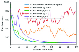
(a)

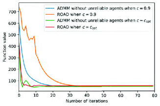
(b)

Figure 1: (a) Performance comparison with different noise intensities. (b) Performance comparison with different choices of algorithm parameter.

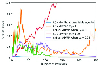
(a)

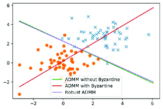
(b)

Figure 2: (a) Performance comparison with different noise intensities. (b) Classification with unreliable agents.

5.1 Decentralized Regression

First, we present the experimental results for a decentralized linear regression problem. The algorithm is deployed to minimize the following mean square error,

$$\min_{\mathbf{x}=\tilde{\mathbf{x}}\in\mathds{R}^{3}}\sum_{i=1}^{D}\frac{1}{2}\|\mathbf{y}_{i}-\mathbf{B}_{i}\mathbf{x}\|^{2}_{2}.$$

For comparison, we use the same experiment setting as that in [13]. Here $\mathbf{x}\in\mathds{R}^{3}$ is the parameter to be estimated and it is generated by normal distribution $\mathcal{N}(\mathbf{0},\mathbf{I})$, $\mathbf{B}_{i}\in\mathds{R}^{3\times 3}$ is the measurement matrix of node $i$ and its elements follow $\mathcal{N}(0,1)$, and $\mathbf{y}_{i}\in\mathds{R}^{3}$ is the linear measurement vector, which is, however, corrupted by Gaussian noise $\mathcal{N}(\mathbf{0},\mathbf{I})$. Note that the cost function is strongly convex and $L$-smooth, and we find that condition (9) is satisfied by the network. We record the cost function value over different iterations.

In Figure $1$(a), we compare the performance of original ADMM [13] with ROAD in the presence of unreliable agents. We set the noise variance for unreliable agents as $\sigma_{b}^{2}=1.5^{2}$ and give results for different noise intensities, i.e., $\mu_{b}$. We can see that if there are no unreliable agents in the network, the ADMM converges quickly to the minimizer. However, in the presence of unreliable agents, with $\mu_{b}=0.5$ and $\mu_{b}=1$, it can be seen that the performance of the original ADMM degrades significantly. We observe that original ADMM approaches a neighborhood of the minimizer whose size depends on the intensities ($\mu_{b}$) of the noise. On the other hand, ROAD achieves a comparable convergence speed as ADMM without error.

Next, we employ the derived optimal choice of the algorithm parameter $c$ and show the performance comparison. The optimal $c$, which is termed as $c_{opt}$, is given in Theorem 4. We compare the performance of the ROAD in the cases where $c=0.9$ and $c=c_{opt}$. We can see clearly from Figure $1$(b) that with the optimal $c$, ROAD achieves a much faster convergence speed. Even though the optimal algorithm parameter is derived for the situation where there are unreliable nodes, the original ADMM can also obtain an acceleration with the optimal $c$.

5.2 Decentralized Classification

Consider a binary classification problem with a support vector machine, and the local cost function is

$$f_{i}(\mathbf{w}_{i},b_{i})=\frac{1}{2}\|\mathbf{w}_{i}\|^{2}_{2}+C\sum_{j=1}^{N}\max(0,1-y_{j}(\mathbf{w}_{i}^{T}\mathbf{x}_{j}+b_{i})).$$

Here, the training set with $N=1000$ sample points is equally partitioned across $10$ agents. For each training point $\{\mathbf{x}_{j},y_{j}\}$, $\mathbf{x}_{j}\in\mathds{R}^{2}$ is the feature vector, and $y_{j}\in\{-1,1\}$ is the corresponding label. We assume that $\mathbf{x}_{j}$ follows a normal distribution $\mathcal{N}([2.8,2.8]^{T},\mathbf{I})$ when $y_{j}=1$, and $\mathcal{N}(\mathbf{0},\mathbf{I})$ when $y_{j}=-1$, respectively. Locally, the training data is evenly composed of samples from two different distributions. In our experiment, each agent updates$\{\mathbf{w},b\}$, and the whole network tries to reach a final consensus on a globally optimal solution. We choose the regularization parameter $c=0.35$ in our experiment.We model the error injected by unreliable agents with distribution $\mathcal{N}(0,1.5^{2})$.

In Figure $2$(a), we present the objective function value against the number of iterations for different algorithms. We observe that in the absence of unreliable agents, the original ADMM algorithm converges quickly and there are no function value fluctuations. When unreliable agents provide erroneous updates, ADMM algorithm diverges from the minimizer significantly. We can see that when the noise intensity $\mu_{b}$ is larger, the size of the neighborhood is larger. On the other hand, when ROAD is employed, we observe that the algorithm converges to the minimizer which corroborates our theoretical results in Theorem $5$.

We show the classification results by depicting the hyperplane ($\mathbf{w}^{T}\mathbf{x}+b=0$) in Figure $2$(b). When there are unreliable agents, the algorithm learns an “incorrect” classifier as is shown by the red line. By using ROAD, we obtain a classifier which is almost the same as the case where there are no unreliable agents. The slight difference arises because the algorithms stop after the same number of iterations in our experiments, thus, ROAD does not achieve the same accuracy as error-free ADMM.

6 Conclusion

We considered the problem of decentralized learning using ADMM in the presence of unreliable agents. We studied the convergence behavior of the decentralized ADMM algorithm and showed that the ADMM converges to a neighborhood of the solution under certain conditions. We suggested guidelines for network structure design to achieve faster convergence. We also gave several conditions on the errors to obtain exact convergence to the solution. A robust variant of the ADMM algorithm was proposed to enable decentralized learning in the presence of unreliable agents and its convergence to the optima was proved. We also provided experimental results to validate the analysis and showed the effectiveness of the proposed robust scheme. We assumed the convexity of the cost function, and one might follow our lines of analysis for non-convex functions. Extension of the analysis and the algorithm to an asynchronous setting can also be considered.

Supplementary Materials

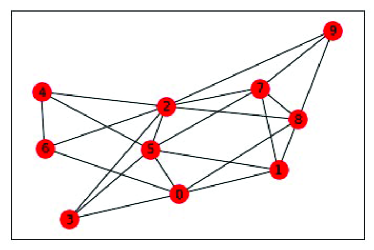
Figure 3: Decentralized network topology.

Lemma 1.

The update of the the algorithm can be written as

$$\mathbf{x}^{k+1}=-\frac{1}{2c}\mathbf{W}^{-1}\nabla f(\mathbf{x}^{k+1})+\frac{\mathbf{W}^{-1}\mathbf{L}_{+}}{2}(\mathbf{x}^{k}+\mathbf{e}^{k})-\frac{\mathbf{W}^{-1}\mathbf{L}_{-}}{2}\left(\sum\limits^{k}_{s=0}\mathbf{x}^{s}+\mathbf{e}^{s}\right).$$ (11)

Proof.

Using the second step of the algorithm, we can write

$$\alpha^{k+1}=\alpha^{k}+c\mathbf{L}_{-}(\mathbf{x}^{k+1}+\mathbf{e}^{k+1})$$ (12)

and

$$\alpha^{k}=\alpha^{k-1}+c\mathbf{L}_{-}(\mathbf{x}^{k}+\mathbf{e}^{k}).$$ (13)

Sum and telescope from iteration 0 to $k$ using (13), and we can get the following by assuming $\alpha^{0}=0$

$$\alpha^{k}=c\mathbf{L}_{-}\sum\limits_{s=0}^{k}\left(\mathbf{x}^{s}+\mathbf{e}^{s}\right).$$ (14)

Substitute the above result to the first step in the algorithm and it yields

$$2c\mathbf{W}\mathbf{x}^{k+1}=-\nabla f(\mathbf{x}^{k+1})+c\mathbf{L}_{+}(\mathbf{x}^{k}+\mathbf{e}^{k})-c\mathbf{L}_{-}\sum\limits_{s=0}^{k}\left(\mathbf{x}^{s}+\mathbf{e}^{s}\right),$$ (15)

which completes the proof. ∎

Lemma 2.

The sequences satisfy

$$\frac{\mathbf{L}_{+}}{2}(\mathbf{z}^{k+1}-\mathbf{z}^{k})-\mathbf{W}\mathbf{e}^{k+1}=-\mathbf{Q}\mathbf{r}^{k+1}-\frac{1}{2c}\nabla f(\mathbf{x}^{k+1})$$ (16)

Proof.

Based on Lemma 1 and the fact $\mathbf{W}=\frac{1}{2}(\mathbf{L}_{-}+\mathbf{L}_{+})$, we can write

$$\mathbf{W}(\mathbf{x}^{k+1}-\mathbf{x}^{k}-\mathbf{e}^{k})+\mathbf{W}(\mathbf{x}^{k}+\mathbf{e}^{k})-\frac{\mathbf{L}_{+}}{2}(\mathbf{x}^{k}+\mathbf{e}^{k})=-\mathbf{Q}\mathbf{r}^{k}-\frac{1}{2c}\nabla f(\mathbf{x}^{k+1}).$$ (17)

Subtracting $\frac{\mathbf{L}_{-}}{2}(\mathbf{x}^{k+1}+\mathbf{e}^{k+1})$ from both sides of the above equation provides

$$\mathbf{W}(\mathbf{x}^{k+1}-\mathbf{x}^{k}-\mathbf{e}^{k})+\frac{\mathbf{L}_{-}}{2}(\mathbf{x}^{k}+\mathbf{e}^{k})-\frac{\mathbf{L}_{-}}{2}(\mathbf{x}^{k+1}+\mathbf{e}^{k+1})=-\mathbf{Q}\mathbf{r}^{k+1}-\frac{1}{2c}\nabla f(\mathbf{x}^{k+1}).$$ (18)

Rearrange and we have the desired result. ∎

Lemma 3.

The null space of $\mathbf{Q}$ null$(\mathbf{Q})$ is span$\{\mathbf{1}\}$.

Proof.

Note that the null space of $\mathbf{Q}$ and $\mathbf{L}_{-}$ are the same. By definition, $\mathbf{L}_{-}=\frac{1}{2}\mathbf{M}_{-}\mathbf{M}_{-}^{T}$ and $\mathbf{M}_{-}=\mathbf{A}_{1}^{T}-\mathbf{A}_{2}^{T}$. Recall that if $(i,j)\in\mathcal{A}$ and $\mathbf{y}_{ij}$ is the $q$th block of $\mathbf{y}$, then the $(q,i)$th block of $\mathbf{A}_{1}$ and the $(q,j)$th block of $\mathbf{A}_{2}$ are $N\times N$ identity matrices $\mathbf{I}_{N}$; otherwise the corresponding blocks are $N\times N$ zero matrices $0_{N}$. Therefore, $\mathbf{M}_{-}^{T}=\mathbf{A}_{1}-\mathbf{A}_{2}$ is a matrix that each row has one “1”, one “-1”, and all zeros otherwise, which means $\mathbf{M}_{-}^{T}\mathbf{1}=\mathbf{0}$, i.e., null$(\mathbf{M}_{-}^{T})$=span$\{\mathbf{1}\}$.

Note that $\mathbf{L}_{-}=\frac{1}{2}\mathbf{M}_{-}\mathbf{M}_{-}^{T}$ and $\mathbf{Q}=\left(\frac{\mathbf{L}_{-}}{2}\right)^{\frac{1}{2}}$, thus null$(\mathbf{Q})$=null$(\mathbf{M}_{-}^{T})$, completing the proof. ∎

Lemma 4.

For some $\mathbf{r}^{\ast}$ that satisfies $\mathbf{Q}\mathbf{r}^{\ast}+\frac{1}{2c}\nabla f(\mathbf{x}^{\ast})=0$ and $\mathbf{r}^{\ast}$ belongs to the column space of $\mathbf{Q}$, the sequences satisfy

$$\frac{\mathbf{L}_{+}}{2}(\mathbf{z}^{k+1}-z^{k})-\mathbf{W}\mathbf{e}^{k+1}=-\mathbf{Q}(\mathbf{r}^{k+1}-\mathbf{r}^{\ast})-\frac{1}{2c}(\nabla f(\mathbf{x}^{k+1})-\nabla f(\mathbf{x}^{\ast}))$$ (19)

Proof.

Using Lemma 2, we have

$$\frac{\mathbf{L}_{+}}{2}(\mathbf{z}^{k+1}-\mathbf{z}^{k})-\mathbf{W}\mathbf{e}^{k+1}=-\mathbf{Q}\mathbf{r}^{k+1}-\frac{1}{2c}\nabla f(\mathbf{x}^{k+1}).$$ (20)

According to Lemma 3, null$(\mathbf{Q})$ is span$\{\mathbf{1}\}$. Since $\mathbf{1}^{T}\nabla f(\mathbf{x}^{\ast})=0$, $\nabla f(\mathbf{x}^{\ast})$ can be written as a linear combination of column vectors of $\mathbf{Q}$. Therefore, there exists $\mathbf{r}$ such that $\frac{1}{2c}\nabla f(x^{\ast})=-\mathbf{Q}\mathbf{r}$. Let $\mathbf{r}^{\ast}$ be the projection of $\mathbf{r}$ onto $\mathbf{Q}$ to obtain $\mathbf{Q}\mathbf{r}=\mathbf{Q}\mathbf{r}^{\ast}$ where $\mathbf{r}^{\ast}$ lies in the column space of $\mathbf{Q}$.

Hence, we can write

$$\frac{\mathbf{L}_{+}}{2}(\mathbf{z}^{k+1}-\mathbf{z}^{k})-\mathbf{W}\mathbf{e}^{k+1}=-\mathbf{Q}(\mathbf{r}^{k+1}-\mathbf{r}^{\ast})-\frac{1}{2c}(\nabla f(\mathbf{x}^{k+1})-\nabla f(\mathbf{x}^{\ast}))$$ (21)

∎

Lemma 5.

$\langle\mathbf{x}^{\ast},\mathbf{Q}\rangle=0.$

Proof.

Since the optimal consensus solution $\mathbf{x}^{\ast}$ has an identical value for all its entries, $\mathbf{x}^{\ast}$ lies in the space spanned by $\mathbf{1}$. Thus, according to Lemma 3, we have the desired result, and also $\langle\mathbf{x}^{\ast},\mathbf{L}_{-}\rangle=0.$ ∎

Appendix A Proof of Theorem 1

Proof.

We prove the first part in Theorem 1. Assuming $f(\mathbf{x})$ is convex, we can have

$$f(\mathbf{x}^{k+1})-f(\mathbf{x}^{\ast})\leq\langle\mathbf{x}^{k+1}-\mathbf{x}^{\ast},\nabla f(x^{k+1})\rangle.$$ (22)

By Lemma 2, it yields

$$f(\mathbf{x}^{k+1})-f(\mathbf{x}^{\ast})\leq \langle\mathbf{x}^{k+1}-\mathbf{x}^{\ast},2c\mathbf{W}\mathbf{e}^{k+1}-2c\mathbf{Q}\mathbf{r}^{k+1}-c\mathbf{L}_{+}(\mathbf{z}^{k+1}-\mathbf{z}^{k})\rangle$$ (23)

$$= \langle\mathbf{x}^{k+1}-\mathbf{x}^{\ast},c\mathbf{L}_{+}(\mathbf{z}^{k}-\mathbf{z}^{k+1})\rangle+\langle\mathbf{x}^{k+1}-\mathbf{x}^{\ast},2c\mathbf{W}\mathbf{e}^{k+1}\rangle$$ (24)

$$+\langle\mathbf{x}^{k+1}-\mathbf{x}^{\ast},-2c\mathbf{Q}\mathbf{r}^{k+1}\rangle$$ (25)

$$= \langle\mathbf{z}^{k+1}-\mathbf{z}^{\ast},c\mathbf{L}_{+}(\mathbf{z}^{k}-\mathbf{z}^{k+1})\rangle-\langle\mathbf{e}^{k+1},c\mathbf{L}_{+}(\mathbf{z}^{k}-\mathbf{z}^{k+1})\rangle$$ (26)

$$+\langle\mathbf{z}^{k+1}-\mathbf{z}^{\ast},-2c\mathbf{Q}\mathbf{r}^{k+1}\rangle-\langle\mathbf{e}^{k+1},-2c\mathbf{Q}\mathbf{r}^{k+1}\rangle+\langle\mathbf{e}^{k+1},2c\mathbf{W}(\mathbf{x}^{k+1}-\mathbf{x}^{\ast})\rangle$$ (27)

$$= 2\langle\mathbf{z}^{k+1}-\mathbf{z}^{\ast},\frac{c\mathbf{L}_{+}}{2}(\mathbf{z}^{k}-\mathbf{z}^{k+1})\rangle+2\langle\mathbf{r}^{k}-\mathbf{r}^{k+1},c(\mathbf{r}^{k+1}-\mathbf{r}^{\prime})\rangle$$ (28)

$$+\langle\mathbf{e}^{k+1},c\mathbf{L}_{+}(\mathbf{z}^{k+1}-\mathbf{z}^{k})+2c\mathbf{Q}\mathbf{r}^{k+1}+2c\mathbf{W}(\mathbf{x}^{k+1}-\mathbf{x}^{\ast})\rangle.$$ (29)

If the algorithm stops at $T$-th iteration, then the function value $f(\mathbf{x}^{T})$ is affected by the error $\mathbf{e}^{k}$ with $k=0,1,\ldots,T-1$. Thus, we can set $k=T-1$ and $\mathbf{e}^{T}=\mathbf{0}$ in the above bound, and obtain

$$f(\mathbf{x}^{T})-f(\mathbf{x}^{\ast})\leq \|\mathbf{z}^{T-1}-\mathbf{z}^{\ast}\|^{2}_{\frac{c\mathbf{L}_{+}}{2}}-\|\mathbf{z}^{T}-\mathbf{z}^{\ast}\|^{2}_{\frac{c\mathbf{L}_{+}}{2}}-\|\mathbf{z}^{T-1}-\mathbf{z}^{T}\|^{2}_{\frac{c\mathbf{L}_{+}}{2}}$$ (30)

$$+c\|\mathbf{r}^{T-1}-\mathbf{r}^{\prime}\|^{2}_{2}-c\|\mathbf{r}^{T}-\mathbf{r}^{\prime}\|^{2}_{2}-c\|\mathbf{r}^{T-1}-\mathbf{r}^{T}\|^{2}_{2}$$ (31)

$$\leq \|\mathbf{q}^{T-1}-\mathbf{p}\|^{2}_{{\mathbf{G}}}.$$ (32)

Now we prove the second part in Theorem 1. By convexity, for any $\mathbf{r}\in\mathds{R}^{DN}$, we can have

$$\frac{f(\mathbf{x}^{k+1})-f(\mathbf{x}^{\ast})}{c}+2\mathbf{r}^{\prime}\mathbf{Q}\mathbf{x}^{k+1}$$ (33)

$$\leq \langle\mathbf{x}^{k+1}-\mathbf{x}^{\ast},-\mathbf{L}_{+}(\mathbf{x}^{k+1}-\mathbf{x}^{k})-\mathbf{L}_{+}(\mathbf{x}^{k}-\mathbf{z}^{k})-2\mathbf{Q}(\mathbf{r}^{k+1}-\mathbf{r})+\mathbf{L}_{-}(\mathbf{z}^{k+1}-\mathbf{x}^{k+1})\rangle$$ (34)

$$= \langle\mathbf{x}^{k+1}-\mathbf{x}^{\ast},\mathbf{L}_{+}(\mathbf{x}^{k}-\mathbf{x}^{k+1})\rangle+\langle\mathbf{x}^{k+1}-\mathbf{x}^{\ast},\mathbf{L}_{+}(\mathbf{z}^{k}-\mathbf{x}^{k})\rangle+\langle\mathbf{x}^{k+1}-\mathbf{x}^{\ast},2\mathbf{Q}(\mathbf{r}-\mathbf{r}^{k+1})\rangle$$ (35)

$$+\langle\mathbf{x}^{k+1}-\mathbf{x}^{\ast},\mathbf{L}_{-}(\mathbf{z}^{k+1}-\mathbf{x}^{k+1})\rangle$$ (36)

$$= \langle\mathbf{x}^{k+1}-\mathbf{x}^{\ast},\mathbf{L}_{+}(\mathbf{x}^{k}-\mathbf{x}^{k+1})\rangle+\langle\mathbf{x}^{k+1}-\mathbf{x}^{\ast},\mathbf{L}_{+}(\mathbf{z}^{k}-\mathbf{x}^{k})\rangle+\langle\mathbf{z}^{k+1}-\mathbf{x}^{\ast},2\mathbf{Q}(\mathbf{r}-\mathbf{r}^{k+1})\rangle$$ (37)

$$+\langle\mathbf{x}^{k+1}-\mathbf{x}^{\ast},\mathbf{L}_{-}(\mathbf{z}^{k+1}-\mathbf{x}^{k+1})\rangle+\langle\mathbf{e}^{k+1},2\mathbf{Q}(\mathbf{r}^{k+1}-\mathbf{r})\rangle$$ (38)

$$= \langle\mathbf{x}^{k+1}-\mathbf{x}^{\ast},\mathbf{L}_{+}(\mathbf{x}^{k}-\mathbf{x}^{k+1})\rangle+\langle\mathbf{x}^{k+1}-\mathbf{x}^{\ast},\mathbf{L}_{+}(\mathbf{z}^{k}-\mathbf{x}^{k})\rangle+\langle\mathbf{r}^{k+1}-\mathbf{r}^{k},2(\mathbf{r}-\mathbf{r}^{k+1})\rangle$$ (39)

$$+\langle\mathbf{x}^{k+1}-\mathbf{x}^{\ast},\mathbf{L}_{-}(\mathbf{z}^{k+1}-\mathbf{x}^{k+1})\rangle+\langle\mathbf{e}^{k+1},2\mathbf{Q}(\mathbf{r}^{k+1}-\mathbf{r})\rangle$$ (40)

$$= \frac{1}{c}(\|\mathbf{p}^{k}-\mathbf{p}\|^{2}_{\mathbf{G}}-\|\mathbf{p}^{k+1}-\mathbf{p}\|^{2}_{\mathbf{G}}-\|\mathbf{p}^{k+1}-\mathbf{p}^{k}\|^{2}_{\mathbf{G}})+\langle\mathbf{x}^{k+1}-\mathbf{x}^{\ast},\mathbf{L}_{+}(\mathbf{z}^{k}-\mathbf{x}^{k})\rangle$$ (41)

$$+\langle\mathbf{x}^{k+1}-\mathbf{x}^{\ast},\mathbf{L}_{-}(\mathbf{z}^{k+1}-\mathbf{x}^{k+1})\rangle+\langle\mathbf{e}^{k+1},2\mathbf{Q}(\mathbf{r}^{k+1}-\mathbf{r})\rangle$$ (42)

$$= \frac{1}{c}(\|\mathbf{p}^{k}-\mathbf{p}\|^{2}_{\mathbf{G}}-\|\mathbf{p}^{k+1}-\mathbf{p}\|^{2}_{\mathbf{G}})-\|\mathbf{Q}\mathbf{x}^{k+1}\|_{2}^{2}-\|\mathbf{Q}\mathbf{e}^{k+1}\|_{2}^{2}+2\langle\frac{\mathbf{L}_{+}}{2}(\mathbf{x}^{k+1}-\mathbf{x}^{\ast}),\mathbf{z}^{k}-\mathbf{x}^{k}\rangle$$ (43)

$$+\langle\mathbf{e}^{k+1},2\mathbf{Q}(\mathbf{r}^{k+1}-\mathbf{r})\rangle$$ (44)

$$= \frac{1}{c}(\|\mathbf{p}^{k}-\mathbf{p}\|^{2}_{\mathbf{G}}-\|\mathbf{p}^{k+1}-\mathbf{p}\|^{2}_{\mathbf{G}})-\frac{\sigma_{\min}(\mathbf{L}_{-})}{2}\|\mathbf{x}^{k+1}-\mathbf{x}^{\ast}\|_{2}^{2}-\|\mathbf{Q}\mathbf{e}^{k+1}\|_{2}^{2}$$ (45)

$$+\frac{1}{\alpha}\|\frac{\mathbf{L}_{+}}{2}(\mathbf{x}^{k+1}-\mathbf{x}^{\ast})\|^{2}_{2}+\alpha\|\mathbf{z}^{k}-\mathbf{x}^{k}\|^{2}_{2}+\langle\mathbf{e}^{k+1},2\mathbf{Q}(\mathbf{r}^{k+1}-\mathbf{r})\rangle$$ (46)

$$\mathrel{\stackrel{{\scriptstyle\makebox[0.0pt]{\mbox{{$\alpha=\frac{\sigma^{2}_{\max}(\mathbf{L}_{+})}{2\sigma_{\min}(\mathbf{L}_{-})}$}}}}}{{=}}} \quad\quad\quad\frac{1}{c}(\|\mathbf{p}^{k}-\mathbf{p}\|^{2}_{\mathbf{G}}-\|\mathbf{p}^{k+1}-\mathbf{p}\|^{2}_{\mathbf{G}})-\|\mathbf{Q}\mathbf{e}^{k+1}\|_{2}^{2}+\frac{\sigma^{2}_{\max}(\mathbf{L}_{+})}{2\sigma_{\min}(\mathbf{L}_{-})}\|\mathbf{z}^{k}-\mathbf{x}^{k}\|^{2}_{2}$$ (47)

$$+\langle\mathbf{e}^{k+1},2\mathbf{Q}(\mathbf{r}^{k+1}-\mathbf{r})\rangle$$ (48)

$$\leq \frac{1}{c}(\|\mathbf{p}^{k}-\mathbf{p}\|^{2}_{\mathbf{G}}-\|\mathbf{p}^{k+1}-\mathbf{p}\|^{2}_{\mathbf{G}})+\frac{\sigma^{2}_{\max}(\mathbf{L}_{+})}{2\sigma_{\min}(\mathbf{L}_{-})}\|\mathbf{e}^{k}\|^{2}_{2}+\langle\mathbf{e}^{k+1},2\mathbf{Q}(\mathbf{r}^{k+1}-\mathbf{r})\rangle.$$ (49)

By letting $\mathbf{r}=0$, telescope and sum from $k=0$ to $T-1$ (the error for the last iteration $\mathbf{e}^{T}=0$), and we obtain

$$\frac{1}{c}\sum_{k=1}^{T}\left(f(\mathbf{x}^{k})-f(\mathbf{x}^{\ast})\right)\leq\frac{1}{c}\|\mathbf{p}^{0}-\mathbf{p}\|^{2}_{\mathbf{G}}+\sum_{k=0}^{T-1}\left(\frac{\sigma^{2}_{\max}(\mathbf{L}_{+})}{2\sigma_{\min}(\mathbf{L}_{-})}\|\mathbf{e}^{k}\|^{2}_{2}+\langle\mathbf{e}^{k},2\mathbf{Q}\mathbf{r}^{k})\rangle\right).$$ (50)

Rearrange and we have the desired result. ∎

Appendix B Proof of Theorem 2

Proof.

By $v$-strong convexity, we obtain

$${v}\|\mathbf{x}^{k+1}-\mathbf{x}^{\ast}\|_{2}^{2}\leq \langle\mathbf{x}^{k+1}-\mathbf{x}^{\ast},\nabla f(\mathbf{x}^{k+1})-\nabla f(\mathbf{x}^{\ast})\rangle$$ (51)

$$= \langle\mathbf{x}^{k+1}-\mathbf{x}^{\ast},c\mathbf{L}_{+}(\mathbf{z}^{k}-\mathbf{z}^{k+1})+2c\mathbf{W}\mathbf{e}^{k+1}-2c\mathbf{Q}(\mathbf{r}^{k+1}-\mathbf{r}^{\ast})\rangle$$ (52)

$$= \langle\mathbf{x}^{k+1}-\mathbf{x}^{\ast},c\mathbf{L}_{+}(\mathbf{z}^{k}-\mathbf{z}^{k+1})\rangle+\langle\mathbf{x}^{k+1}-\mathbf{x}^{\ast},2c\mathbf{W}\mathbf{e}^{k+1}\rangle$$ (53)

$$+\langle\mathbf{x}^{k+1}-\mathbf{x}^{\ast},-2c\mathbf{Q}(\mathbf{r}^{k+1}-\mathbf{r}^{\ast})\rangle$$ (54)

$$= \langle\mathbf{z}^{k+1}-\mathbf{z}^{\ast},c\mathbf{L}_{+}(\mathbf{z}^{k}-\mathbf{z}^{k+1})\rangle-\langle\mathbf{e}^{k+1},c\mathbf{L}_{+}(\mathbf{z}^{k}-\mathbf{z}^{k+1})\rangle$$ (55)

$$+\langle\mathbf{x}^{k+1}+\mathbf{e}^{k+1}-\mathbf{x}^{\ast},-2c\mathbf{Q}(\mathbf{r}^{k+1}-\mathbf{r}^{\ast})\rangle$$ (56)

$$-\langle\mathbf{e}^{k+1},-2c\mathbf{Q}(\mathbf{r}^{k+1}-\mathbf{r}^{\ast})\rangle+\langle\mathbf{e}^{k+1},2c\mathbf{W}(\mathbf{x}^{k+1}-\mathbf{x}^{\ast})\rangle$$ (57)

$$= 2\langle\mathbf{z}^{k+1}-\mathbf{z}^{\ast},\frac{c\mathbf{L}_{+}}{2}(\mathbf{z}^{k}-\mathbf{z}^{k+1})\rangle+2\langle\mathbf{r}^{k}-\mathbf{r}^{k+1},c(\mathbf{r}^{k+1}-\mathbf{r}^{\ast})\rangle$$ (58)

$$+\langle\mathbf{e}^{k+1},c\mathbf{L}_{+}(\mathbf{z}^{k+1}-\mathbf{z}^{k})+2c\mathbf{Q}(\mathbf{r}^{k+1}-\mathbf{r}^{\ast})+2c\mathbf{W}(\mathbf{x}^{k+1}-\mathbf{x}^{\ast})\rangle$$ (59)

$$= \|\mathbf{q}^{k}-\mathbf{q}^{\ast}\|^{2}_{\mathbf{G}}-\|\mathbf{q}^{k+1}-\mathbf{q}^{\ast}\|^{2}_{\mathbf{G}}-\|\mathbf{q}^{k}-\mathbf{q}^{k+1}\|^{2}_{\mathbf{G}}$$ (60)

$$+\langle\mathbf{e}^{k+1},c\mathbf{L}_{+}(\mathbf{z}^{k+1}-\mathbf{z}^{k})+2c\mathbf{Q}(\mathbf{r}^{k+1}-\mathbf{r}^{\ast})+2c\mathbf{W}(\mathbf{x}^{k+1}-\mathbf{x}^{\ast})\rangle$$ (61)

For any $\lambda>0$, using the basic inequality

$$\|\mathbf{a}+\mathbf{b}\|^{2}_{2}+(\lambda-1)\|\mathbf{a}\|_{2}^{2}\geq(1-\frac{1}{\lambda})\|\mathbf{b}\|_{2}^{2}$$ (62)

we can write for $\lambda_{1}>1$ and $\lambda_{2}>1$

$$\frac{\sigma_{\max}^{2}(\mathbf{L}_{+})}{4}\|\mathbf{z}^{k+1}-\mathbf{z}^{k}\|^{2}_{2}+\frac{(\lambda_{1}-1)L^{2}\|\mathbf{x}^{k+1}-\mathbf{x}^{\ast}\|^{2}_{2}}{4c^{2}}$$ (63)

$$\geq\|\frac{\mathbf{L}_{+}}{2}(\mathbf{z}^{k+1}-\mathbf{z}^{k})\|^{2}_{2}+(\lambda_{1}-1)\|\frac{1}{2c}\left(\nabla f(\mathbf{x}^{k+1})-\nabla f(\mathbf{x}^{\ast})\right)\|^{2}_{2}$$ (64)

$$\geq\left(1-\frac{1}{\lambda_{1}}\right)\|\mathbf{W}\mathbf{e}^{k+1}-\mathbf{Q}(\mathbf{r}^{k+1}-\mathbf{r}^{\ast})\|^{2}_{2}$$ (65)

$$\geq\left(1-\frac{1}{\lambda_{1}}\right)(1-\frac{1}{\lambda_{2}})\|\mathbf{Q}(\mathbf{r}^{k+1}-\mathbf{r}^{\ast})\|^{2}_{2}-\left(1-\frac{1}{\lambda_{1}}\right)(\lambda_{2}-1)\|\mathbf{W}\mathbf{e}^{k+1}\|^{2}_{2}$$ (66)

$$\geq\left(1-\frac{1}{\lambda_{1}}\right)(1-\frac{1}{\lambda_{2}})\sigma^{2}_{\min}(\mathbf{Q})\|\mathbf{r}^{k+1}-\mathbf{r}^{\ast}\|^{2}_{2}-\left(1-\frac{1}{\lambda_{1}}\right)(\lambda_{2}-1)\sigma^{2}_{\max}(\mathbf{W})\|\mathbf{e}^{k+1}\|^{2}_{2}.$$ (67)

Thus, for a positive quantity $\delta$,

$$\frac{\delta\sigma_{\max}^{2}(\mathbf{L}_{+})\lambda_{1}\lambda_{2}}{4\sigma^{2}_{\min}(\mathbf{Q})(\lambda_{1}-1)(\lambda_{2}-1)}\|\mathbf{z}^{k+1}-\mathbf{z}^{k}\|^{2}_{2}+\frac{\delta\lambda_{1}\lambda_{2}L^{2}\|\mathbf{x}^{k+1}-\mathbf{x}^{\ast}\|^{2}_{2}}{4c^{2}\sigma^{2}_{\min}(\mathbf{Q})(\lambda_{2}-1)}$$ (68)

$$\geq\delta\|\mathbf{r}^{k+1}-\mathbf{r}^{\ast}\|^{2}_{2}-\frac{\delta\lambda_{2}\sigma^{2}_{\max}(\mathbf{W})}{\sigma^{2}_{\min}(\mathbf{Q})}\|\mathbf{e}^{k+1}\|^{2}_{2}.$$ (69)

Since $\mathbf{x}^{k+1}-\mathbf{x}^{\ast}=\mathbf{z}^{k+1}-\mathbf{z}^{\ast}-\mathbf{e}^{k+1}$, for any $\lambda_{3}>1$, we can get

$$\|\mathbf{x}^{k+1}-\mathbf{x}^{\ast}\|^{2}_{2}\geq\left(1-\frac{1}{\lambda_{3}}\right)\|\mathbf{z}^{k+1}-\mathbf{z}^{\ast}\|^{2}_{2}-\left(\lambda_{3}-1\right)\|\mathbf{e}^{k+1}\|^{2}_{2}.$$ (70)

Therefore, the addition of (68)$\times c^{2}$ and (70)$\times\frac{\delta c^{2}\sigma^{2}_{\max}(L_{+})\lambda_{3}}{4(\lambda_{3}-1)}$ yields

$$\frac{c^{2}\delta\sigma_{\max}^{2}(\mathbf{L}_{+})\lambda_{1}\lambda_{2}}{4\sigma^{2}_{\min}(\mathbf{Q})(\lambda_{1}-1)(\lambda_{2}-1)}\|\mathbf{z}^{k+1}-\mathbf{z}^{k}\|^{2}_{2}+\left(\frac{\delta\lambda_{1}\lambda_{2}L^{2}}{4\sigma^{2}_{\min}(\mathbf{Q})(\lambda_{2}-1)}+\frac{\delta c^{2}\sigma^{2}_{\max}(\mathbf{L}_{+})\lambda_{3}}{4(\lambda_{3}-1)}\right)\|\mathbf{x}^{k+1}-\mathbf{x}^{\ast}\|^{2}_{2}$$ (71)

$$\geq\delta c^{2}\|\mathbf{r}^{k+1}-\mathbf{r}^{\ast}\|^{2}_{2}+\frac{\delta c^{2}\sigma^{2}_{\max}(\mathbf{L}_{+})}{4}\|\mathbf{z}^{k+1}-\mathbf{z}^{k}\|^{2}_{2}-\left(\frac{c^{2}\delta\lambda_{2}\sigma^{2}_{\max}(\mathbf{W})}{\sigma^{2}_{\min}(\mathbf{Q})}+\frac{\delta c^{2}\sigma^{2}_{\max}(\mathbf{L}_{+})\lambda_{3}}{4}\right)\|\mathbf{e}^{k+1}\|^{2}_{2}$$ (72)

$$\geq\delta\|c(\mathbf{r}^{k+1}-\mathbf{r}^{\ast})\|^{2}_{2}+\delta\|\frac{c\mathbf{L}_{+}}{2}(\mathbf{z}^{k+1}-\mathbf{z}^{k})\|^{2}_{2}-\left(\frac{c^{2}\delta\lambda_{2}\sigma^{2}_{\max}(\mathbf{W})}{\sigma^{2}_{\min}(\mathbf{Q})}+\frac{\delta c^{2}\sigma^{2}_{\max}(\mathbf{L}_{+})\lambda_{3}}{4}\right)\|\mathbf{e}^{k+1}\|^{2}_{2}$$ (73)

$$=\delta\|\mathbf{q}^{k+1}-\mathbf{q}^{\ast}\|^{2}_{\mathbf{G}}-\left(\frac{c^{2}\delta\lambda_{2}\sigma^{2}_{\max}(\mathbf{W})}{\sigma^{2}_{\min}(\mathbf{Q})}+\frac{\delta c^{2}\sigma^{2}_{\max}(\mathbf{L}_{+})\lambda_{3}}{4}\right)\|\mathbf{e}^{k+1}\|^{2}_{2}.$$ (74)

Choose $\delta$ to be such that

$$\frac{c^{2}\delta\sigma_{\max}^{2}(\mathbf{L}_{+})\lambda_{1}\lambda_{2}}{4\sigma^{2}_{\min}(\mathbf{Q})(\lambda_{1}-1)(\lambda_{2}-1)} \leq\frac{c^{2}\sigma^{2}_{\min}\mathbf{(}\mathbf{L}_{+})}{4}$$ (75)

$$\left(\frac{\delta\lambda_{1}\lambda_{2}L^{2}}{4\sigma^{2}_{\min}(\mathbf{Q})(\lambda_{2}-1)}+\frac{\delta c^{2}\sigma^{2}_{\max}(\mathbf{L}_{+})\lambda_{3}}{4(\lambda_{3}-1)}\right) \leq v,$$ (76)

and we can have

$$\frac{c^{2}\sigma^{2}_{\min}(\mathbf{L}_{+})}{4}\|\mathbf{z}^{k+1}-\mathbf{z}^{k}\|^{2}_{2}+v\|\mathbf{x}^{k+1}-\mathbf{x}^{k}\|^{2}_{2}\geq$$ (77)

$$\delta\|\mathbf{q}^{k+1}-\mathbf{q}^{\ast}\|^{2}_{\mathbf{G}}-\left(\frac{c^{2}\delta\lambda_{2}\sigma^{2}_{\max}(\mathbf{W})}{\sigma^{2}_{\min}(\mathbf{Q})}+\frac{\delta c^{2}\sigma^{2}_{\max}(\mathbf{L}_{+})\lambda_{3}}{4}\right)\|\mathbf{e}^{k+1}\|^{2}_{2}.$$ (78)

Thus, it is straightforward to write

$$\|\mathbf{q}^{k+1}-\mathbf{q}^{k}\|_{\mathbf{G}}^{2}+v\|\mathbf{x}^{k+1}-\mathbf{x}^{k}\|^{2}_{2}$$ (79)

$$\geq\|c(\mathbf{r}^{k+1}-\mathbf{r}^{k})\|^{2}_{2}+\|\frac{c\mathbf{L}_{+}}{2}(\mathbf{z}^{k+1}-\mathbf{z}^{k})\|^{2}_{2}+v\|\mathbf{x}^{k+1}-\mathbf{x}^{k}\|^{2}_{2}$$ (80)

$$\geq c^{2}\|\mathbf{r}^{k+1}-\mathbf{r}^{k}\|^{2}_{2}+\frac{c^{2}\sigma^{2}_{\min}(\mathbf{L}_{+})}{4}\|\mathbf{z}^{k+1}-\mathbf{z}^{k}\|^{2}_{2}+v\|\mathbf{x}^{k+1}-\mathbf{x}^{k}\|^{2}_{2}$$ (81)

$$\geq c^{2}\|\mathbf{r}^{k+1}-\mathbf{r}^{k}\|^{2}_{2}+\delta\|\mathbf{q}^{k+1}-\mathbf{q}^{\ast}\|^{2}_{\mathbf{G}}-\left(\frac{c^{2}\delta\lambda_{2}\sigma^{2}_{\max}(\mathbf{W})}{\sigma^{2}_{\min}(\mathbf{Q})}+\frac{\delta c^{2}\sigma^{2}_{\max}(\mathbf{L}_{+})\lambda_{3}}{4}\right)\|\mathbf{e}^{k+1}\|^{2}_{2}.$$ (82)

Recall the result in (51) regarding the bound to $v\|\mathbf{x}^{k+1}-\mathbf{x}^{k}\|^{2}_{2}$, and we can further write

$$\|\mathbf{q}^{k}-\mathbf{q}^{\ast}\|^{2}_{\mathbf{G}}-\|\mathbf{q}^{k+1}-\mathbf{q}^{\ast}\|^{2}_{\mathbf{G}}$$ (83)

$$+\langle\mathbf{e}^{k+1},c\mathbf{L}_{+}(\mathbf{z}^{k+1}-\mathbf{z}^{k})+2c\mathbf{Q}(\mathbf{r}^{k+1}-\mathbf{r}^{\ast})+2c\mathbf{W}(\mathbf{x}^{k+1}-\mathbf{x}^{\ast})\rangle$$ (84)

$$\geq\delta\|\mathbf{q}^{k+1}-\mathbf{q}^{\ast}\|^{2}_{\mathbf{G}}-\left(\frac{c^{2}\delta\lambda_{2}\sigma^{2}_{\max}(\mathbf{W})}{\sigma^{2}_{\min}(\mathbf{Q})}+\frac{\delta c^{2}\sigma^{2}_{\max}(\mathbf{L}_{+})\lambda_{3}}{4}\right)\|\mathbf{e}^{k+1}\|^{2}_{2}$$ (85)

Let $P=\frac{c^{2}\delta\lambda_{2}\sigma^{2}_{\max}(\mathbf{W})}{\sigma^{2}_{\min}(\mathbf{Q})}+\frac{\delta c^{2}\sigma^{2}_{\max}(\mathbf{L}_{+})\lambda_{3}}{4}$. Rearrange the expression and we get

$$\|\mathbf{q}^{k+1}-\mathbf{q}^{\ast}\|^{2}_{\mathbf{G}}\leq \frac{\|\mathbf{q}^{k}-\mathbf{q}^{\ast}\|^{2}_{\mathbf{G}}}{1+\delta}+\frac{P}{1+\delta}\|\mathbf{e}^{k+1}\|^{2}_{2}$$ (86)

$$+\frac{1}{1+\delta}\langle\mathbf{e}^{k+1},c\mathbf{L}_{+}(\mathbf{z}^{k+1}-\mathbf{z}^{k})+2c\mathbf{Q}(\mathbf{r}^{k+1}-\mathbf{r}^{\ast})+2c\mathbf{W}(\mathbf{x}^{k+1}-\mathbf{x}^{\ast})\rangle$$ (87)

∎

Lemma 6.

Let $\beta\in(0,\frac{1+\delta}{4})$, $b\in(0,1)$, $\lambda_{4}>1$, and then we have

$$(1-b)\left(\frac{1}{4}-\frac{\beta}{1+\delta}\right)\sigma_{\min}^{2}(\mathbf{L}_{+})\|\mathbf{z}^{k+1}-\mathbf{z}^{\ast}\|^{2}_{2}+\left(1-\frac{4\beta}{1+\delta}\right)\|\mathbf{r}^{k+1}-\mathbf{r}^{\ast}\|^{2}_{2}$$ (88)

$$+b\left(\frac{1}{4}-\frac{\beta}{1+\delta}\right)\sigma_{\min}^{2}(\mathbf{L}_{+})\left(1-\frac{1}{\lambda_{4}}\right)\|\mathbf{x}^{k+1}-\mathbf{x}^{\ast}\|^{2}_{2}$$ (89)

$$\leq\frac{1/4+\beta}{1+\delta}\sigma^{2}_{\max}(\mathbf{L}_{+})\|\mathbf{z}^{k}-\mathbf{z}^{\ast}\|^{2}_{2}+\frac{1}{1+\delta}\|\mathbf{r}^{k}-\mathbf{r}^{\ast}\|^{2}_{2}$$ (90)

$$+\left[\frac{P+1/2\beta}{(1+\delta)c^{2}}+b\left(\frac{1}{4}-\frac{\beta}{1+\delta}\right)\sigma_{\min}^{2}(\mathbf{L}_{+})(\lambda_{4}-1)\right]\|\mathbf{e}^{k+1}\|^{2}_{2}$$ (91)

$$+\frac{4\beta\sigma^{2}_{\max}(\mathbf{W})}{1+\delta}\|\mathbf{x}^{k+1}-\mathbf{x}^{\ast}\|^{2}_{2}.$$ (92)

Proof.

First, we rewrite the result in Lemma 2 in the following form

$$\|\frac{c\mathbf{L}_{+}}{2}(\mathbf{z}^{k+1}-\mathbf{z}^{\ast})\|^{2}_{2}+\|c(\mathbf{r}^{k+1}-\mathbf{r}^{\ast})\|^{2}_{2}\leq\frac{1}{1+\delta}\left(\|\frac{c\mathbf{L}_{+}}{2}(\mathbf{z}^{k}-\mathbf{z}^{\ast})\|^{2}_{2}+\|c(\mathbf{r}^{k}-\mathbf{r}^{\ast})\|^{2}_{2}\right)$$ (93)

$$+\frac{P}{1+\delta}\|\mathbf{e}^{k+1}\|^{2}_{2}+\frac{1}{1+\sigma}\langle\mathbf{e}^{k+1},c\mathbf{L}_{+}(\mathbf{z}^{k+1}-\mathbf{z}^{k})+2c\mathbf{Q}(\mathbf{r}^{k+1}-\mathbf{r}^{\ast})+2c\mathbf{W}(\mathbf{x}^{k+1}-\mathbf{x}^{\ast})\rangle$$ (94)

$$\leq\frac{1}{1+\delta}\left(\|\frac{c\mathbf{L}_{+}}{2}(\mathbf{z}^{k}-\mathbf{z}^{\ast})\|^{2}_{2}+\|c(\mathbf{r}^{k}-\mathbf{r}^{\ast})\|^{2}_{2}\right)+\left(\frac{P}{1+\delta}+\frac{1/2\beta}{1+\delta}\right)\|\mathbf{e}^{k+1}\|^{2}_{2}$$ (95)

$$+\frac{\beta}{1+\delta}\|\frac{c\mathbf{L}_{+}}{2}(\mathbf{z}^{k+1}-\mathbf{z}^{k})+c\mathbf{Q}(\mathbf{r}^{k+1}-\mathbf{r}^{\ast})+c\mathbf{W}(\mathbf{x}^{k+1}-\mathbf{x}^{\ast})\|^{2}_{2}$$ (96)

$$\leq\frac{1}{1+\delta}\left(\|\frac{c\mathbf{L}_{+}}{2}(\mathbf{z}^{k}-\mathbf{z}^{\ast})\|^{2}_{2}+\|c(\mathbf{r}^{k}-\mathbf{r}^{\ast})\|^{2}_{2}\right)+\left(\frac{P}{1+\delta}+\frac{1/2\beta}{1+\delta}\right)\|\mathbf{e}^{k+1}\|^{2}_{2}$$ (97)

$$+\frac{\beta}{1+\delta}\|\frac{c\mathbf{L}_{+}}{2}(\mathbf{z}^{k+1}-\mathbf{z}^{k})+c\mathbf{Q}(\mathbf{r}^{k+1}-\mathbf{r}^{\ast})+c\mathbf{W}(\mathbf{x}^{k+1}-\mathbf{x}^{\ast})\|^{2}_{2}$$ (98)

$$\leq\frac{1}{1+\delta}\left(\|\frac{c\mathbf{L}_{+}}{2}(\mathbf{z}^{k}-\mathbf{z}^{\ast})\|^{2}_{2}+\|c(\mathbf{r}^{k}-\mathbf{r}^{\ast})\|^{2}_{2}\right)+\left(\frac{P}{1+\delta}+\frac{1/2\beta}{1+\delta}\right)\|\mathbf{e}^{k+1}\|^{2}_{2}$$ (99)

$$+\frac{4\beta}{1+\delta}\|\frac{c\mathbf{L}_{+}}{2}(\mathbf{z}^{k+1}-\mathbf{z}^{\ast})\|^{2}_{2}+\frac{4\alpha}{1+\delta}\|\frac{c\mathbf{L}_{+}}{2}(\mathbf{z}^{k}-\mathbf{z}^{\ast})\|^{2}_{2}$$ (100)

$$+\frac{4\beta}{1+\delta}\|c\mathbf{Q}(\mathbf{r}^{k+1}-\mathbf{r}^{\ast})\|^{2}_{2}+\frac{4\beta}{1+\delta}\|c\mathbf{W}(\mathbf{x}^{k+1}-\mathbf{x}^{\ast})\|^{2}_{2}$$ (101)

where $\beta>0$.

Rearranging the inequality provides

$$\left(1-\frac{4\beta}{1+\delta}\right)\|\frac{c\mathbf{L}_{+}}{2}(\mathbf{z}^{k+1}-\mathbf{z}^{\ast})\|^{2}_{2}+\left(1-\frac{4\beta}{1+\delta}\right)\|c(\mathbf{r}^{k+1}-\mathbf{r}^{\ast})\|^{2}_{2}$$ (102)

$$\leq\left(\frac{1}{1+\delta}+\frac{4\beta}{1+\delta}\right)\|\frac{c\mathbf{L}_{+}}{2}(\mathbf{z}^{k}-\mathbf{z}^{\ast})\|^{2}_{2}+\frac{1}{1+\delta}\|c(\mathbf{r}^{k}-\mathbf{r}^{\ast})\|^{2}_{2}$$ (103)

$$+\frac{P+1/2\beta}{1+\delta}\|\mathbf{e}^{k+1}\|^{2}_{2}+\frac{4\beta}{1+\delta}\|c\mathbf{W}(\mathbf{x}^{k+1}-\mathbf{x}^{\ast})\|^{2}_{2}.$$ (104)

Note that the parameters should be chosen such that $\left(1-\frac{4\beta}{1+\delta}\right)>0$.

Then we can write

$$\left(\frac{1}{4}-\frac{\beta}{1+\delta}\right)\sigma_{\min}^{2}(\mathbf{L}_{+})\|\mathbf{z}^{k+1}-\mathbf{z}^{\ast}\|^{2}_{2}+\left(1-\frac{4\beta}{1+\delta}\right)\|\mathbf{r}^{k+1}-\mathbf{r}^{\ast}\|^{2}_{2}$$ (105)

$$\leq\left(\frac{1}{4(1+\delta)}+\frac{\beta}{1+\delta}\right)\sigma^{2}_{\max}(\mathbf{L}_{+})\|\mathbf{z}^{k}-\mathbf{z}^{\ast}\|^{2}_{2}+\frac{1}{1+\delta}\|\mathbf{r}^{k}-\mathbf{r}^{\ast}\|^{2}_{2}$$ (106)

$$+\frac{P+1/2\beta}{(1+\delta)c^{2}}\|\mathbf{e}^{k+1}\|^{2}_{2}+\frac{4\beta\sigma^{2}_{\max}(\mathbf{W})}{1+\delta}\|\mathbf{x}^{k+1}-\mathbf{x}^{\ast}\|^{2}_{2}.$$ (107)

Since we have the inequality $\|\mathbf{z}^{k+1}-\mathbf{z}^{\ast}\|^{2}_{2}\geq\left(1-\frac{1}{\lambda_{4}}\right)\|\mathbf{x}^{k+1}-\mathbf{x}^{\ast}\|^{2}_{2}-(\lambda_{4}-1)\|\mathbf{e}^{k+1}\|^{2}_{2}$, for $b\in(0,1)$, we can get

$$b\left(\frac{1}{4}-\frac{\beta}{1+\delta}\right)\sigma_{\min}^{2}(\mathbf{L}_{+})\|\mathbf{z}^{k+1}-\mathbf{z}^{\ast}\|^{2}_{2}\geq b\left(\frac{1}{4}-\frac{\beta}{1+\delta}\right)\sigma_{\min}^{2}(\mathbf{L}_{+})\left(1-\frac{1}{\lambda_{4}}\right)\|\mathbf{x}^{k+1}-\mathbf{x}^{\ast}\|^{2}_{2}$$ (108)

$$-b\left(\frac{1}{4}-\frac{\beta}{1+\delta}\right)\sigma_{\min}^{2}(\mathbf{L}_{+})(\lambda_{4}-1)\|\mathbf{e}^{k+1}\|^{2}_{2}.$$ (109)

Thus,

$$(1-b)\left(\frac{1}{4}-\frac{\beta}{1+\delta}\right)\sigma_{\min}^{2}(\mathbf{L}_{+})\|\mathbf{z}^{k+1}-\mathbf{z}^{\ast}\|^{2}_{2}+\left(1-\frac{4\beta}{1+\delta}\right)\|\mathbf{r}^{k+1}-\mathbf{r}^{\ast}\|^{2}_{2}$$ (110)

$$+b\left(\frac{1}{4}-\frac{\beta}{1+\delta}\right)\sigma_{\min}^{2}(\mathbf{L}_{+})\left(1-\frac{1}{\lambda_{4}}\right)\|\mathbf{x}^{k+1}-\mathbf{x}^{\ast}\|^{2}_{2}$$ (111)

$$\leq\frac{1/4+\beta}{1+\delta}\sigma^{2}_{\max}(\mathbf{L}_{+})\|\mathbf{z}^{k}-\mathbf{z}^{\ast}\|^{2}_{2}+\frac{1}{1+\delta}\|\mathbf{r}^{k}-\mathbf{r}^{\ast}\|^{2}_{2}$$ (112)

$$+\left[\frac{P+1/2\beta}{(1+\delta)c^{2}}+b\left(\frac{1}{4}-\frac{\beta}{1+\delta}\right)\sigma_{\min}^{2}(\mathbf{L}_{+})(\lambda_{4}-1)\right]\|\mathbf{e}^{k+1}\|^{2}_{2}$$ (113)

$$+\frac{4\beta\sigma^{2}_{\max}(\mathbf{W})}{1+\delta}\|\mathbf{x}^{k+1}-\mathbf{x}^{\ast}\|^{2}_{2}.$$ (114)

∎

Defining

$$A_{1}=\frac{4}{(1-b)\sigma^{2}_{\min}(\mathbf{L}_{+})},$$ (115)

and

$$A_{2}=\frac{4}{(1+4\beta)\sigma^{2}_{\max}(\mathbf{L}_{+})},$$ (116)

we have the desired result.

Appendix C Proof of Theorem 3

C.1 Eliminate $\|\mathbf{x}^{k+1}-\mathbf{x}^{\ast}\|^{2}_{2}$

First, we want to eliminate the term $\|\mathbf{x}^{k+1}-\mathbf{x}^{\ast}\|^{2}_{2}$ in Lemma 6, which requires

$$b\left(\frac{1}{4}-\frac{\beta}{1+\delta}\right)\sigma_{\min}^{2}(\mathbf{L}_{+})\left(1-\frac{1}{\lambda_{4}}\right)\geq\frac{4\beta\sigma^{2}_{\max}(\mathbf{W})}{1+\delta}$$ (117)

and it is equivalent to that

$$\beta\leq\frac{b(1+\delta)\sigma^{2}_{\min}(\mathbf{L}_{+})\left(1-\frac{1}{\lambda_{4}}\right)}{4b\sigma^{2}_{\min}(\mathbf{L}_{+})\left(1-\frac{1}{\lambda_{4}}\right)+16\sigma^{2}_{\max}(\mathbf{W})}$$ (118)

Then we can write

$$(1-b)\left(\frac{1}{4}-\frac{\beta}{1+\delta}\right)\sigma_{\min}^{2}(\mathbf{L}_{+})\|\mathbf{z}^{k+1}-\mathbf{z}^{\ast}\|^{2}_{2}+\left(1-\frac{4\beta}{1+\delta}\right)\|\mathbf{r}^{k+1}-\mathbf{r}^{\ast}\|^{2}_{2}$$ (119)

$$\leq\frac{1/4+\beta}{1+\delta}\sigma^{2}_{\max}(\mathbf{L}_{+})\|\mathbf{z}^{k}-\mathbf{z}^{\ast}\|^{2}_{2}+\frac{1}{1+\delta}\|\mathbf{r}^{k}-\mathbf{r}^{\ast}\|^{2}_{2}$$ (120)

$$+\left[\frac{P+1/2\beta}{(1+\delta)c^{2}}+b\left(\frac{1}{4}-\frac{\beta}{1+\delta}\right)\sigma_{\min}^{2}(\mathbf{L}_{+})(\lambda_{4}-1)\right]\|\mathbf{e}^{k+1}\|^{2}_{2}$$ (121)

which can be further simplified

$$\|\mathbf{z}^{k+1}-\mathbf{z}^{\ast}\|^{2}_{2}+A_{1}\|\mathbf{r}^{k+1}-\mathbf{r}^{\ast}\|^{2}_{2}\leq B(\|\mathbf{z}^{k}-\mathbf{z}^{\ast}\|^{2}_{2}+A_{2}\|\mathbf{r}^{k}-\mathbf{r}^{\ast}\|^{2}_{2})+C\|\mathbf{e}^{k+1}\|^{2}_{2}$$ (123)

We require the following for convergence analysis

$$A_{1}\geq A_{2}$$ (124)

which leads to the requirement

$$(1-b)\sigma^{2}_{\min}(\mathbf{L}_{+})\leq(1+\beta)\sigma^{2}_{\max}(\mathbf{L}_{+}).$$ (125)

Note that this requirement is satisfied intrinsically.

Therefore, we get

$$\|\mathbf{z}^{k+1}-\mathbf{z}^{\ast}\|^{2}_{2}+A_{1}\|\mathbf{r}^{k+1}-\mathbf{r}^{\ast}\|^{2}_{2}\leq B^{k+1}\left(\|\mathbf{z}^{0}-\mathbf{z}^{\ast}\|^{2}_{2}+A_{2}\|\mathbf{r}^{0}-\mathbf{r}^{\ast}\|^{2}_{2}+\sum\limits^{k+1}_{s=1}B^{-s}C\|\mathbf{e}^{s}\|^{2}_{2}\right)$$ (126)

and we have the desired result since $A_{1}\|r^{k+1}-r^{\ast}\|^{2}_{2}>0$.

C.2 $B\in(0,1)$

The above convergence result requires that $B\in(0,1)$. First, having $\beta$ in Theorem 3 at hand, we can make sure that $B$ is greater than 0. Then, it requires that $B<1$ and correspondingly

$${(1+4\beta)\sigma^{2}_{\max}(\mathbf{L}_{+})}\leq{(1-b)(1+\delta-4\beta)\sigma^{2}_{\min}(\mathbf{L}_{+})}$$ (127)

which is equivalent to that

$$\beta\leq\frac{(1-b)(1+\delta)\sigma^{2}_{\min}(\mathbf{L}_{+})-\sigma^{2}_{\max}(\mathbf{L}_{+})}{4\sigma^{2}_{\max}(\mathbf{L}_{+})+4(1-b)\sigma^{2}_{\min}(\mathbf{L}_{+})}$$ (128)

and

$${(1-b)(1+\delta)\sigma^{2}_{\min}(\mathbf{L}_{+})-\sigma^{2}_{\max}(\mathbf{L}_{+})}>0.$$ (129)

Since $b$ can be arbitrarily chosen from $(0,1)$, we also need

$$0<\frac{\sigma^{2}_{\max}(\mathbf{L}_{+})}{(1+\delta)\sigma^{2}_{\min}(\mathbf{L}_{+})}<1$$ (130)

One intuition is that we should design a network such that $\frac{\sigma^{2}_{\max}(\mathbf{L}_{+})}{\sigma^{2}_{\min}(\mathbf{L}_{+})}$ is the smallest possible. Substituting $\delta$ in the expression and we have

$$\frac{\sigma^{2}_{\min}(\mathbf{L}_{+})}{\sigma^{2}_{\max}(\mathbf{L}_{+})}>\frac{L^{2}-2v+\sqrt{(L^{2}+2v)^{2}+16v^{2}\frac{\lambda_{2}-1}{\lambda_{2}}\sigma^{2}_{\min}(\mathbf{Q})}}{4v\frac{\lambda_{2}-1}{\lambda_{2}}\sigma^{2}_{\min}(\mathbf{Q})+2L^{2}}.$$ (131)

Appendix D Proof of Theorem 4

Note that $\delta$ is chosen as

$$\delta=\min\left\{\frac{(\lambda_{1}-1)(\lambda_{2}-1)\sigma^{2}_{\min}(\mathbf{Q})\sigma^{2}_{\min}(\mathbf{L}_{+})}{\lambda_{1}\lambda_{2}\sigma^{2}_{\max}(\mathbf{L}_{+})},\frac{4v(\lambda_{2}-1)(\lambda_{3}-1)\sigma^{2}_{\min}(\mathbf{Q})}{\lambda_{1}\lambda_{2}(\lambda_{3}-1)L^{2}+c^{2}\lambda_{3}(\lambda_{2}-1)\sigma^{2}_{\max}(\mathbf{L}_{+})\sigma^{2}_{\min}(\mathbf{Q})}\right\}$$ (132)

We choose $c$ such that

$$\lambda_{1}\lambda_{2}(\lambda_{3}-1)L^{2}=c^{2}\lambda_{3}(\lambda_{2}-1)\sigma^{2}_{\max}(\mathbf{L}_{+})\sigma^{2}_{\min}(\mathbf{Q}),$$ (133)

which yields

$$c=\sqrt[]{\frac{\lambda_{1}\lambda_{2}(\lambda_{3}-1)L^{2}}{\lambda_{3}(\lambda_{2}-1)\sigma^{2}_{\max}(\mathbf{L}_{+})\sigma^{2}_{\min}(\mathbf{Q})}}$$ (134)

and

$$\delta= \min\left\{\frac{(\lambda_{1}-1)(\lambda_{2}-1)\sigma^{2}_{\min}(\mathbf{Q})\sigma^{2}_{\min}(\mathbf{L}_{+})}{\lambda_{1}\lambda_{2}\sigma^{2}_{\max}(\mathbf{L}_{+})},\frac{2v(\lambda_{2}-1)\sigma^{2}_{\min}(\mathbf{Q})}{\lambda_{1}\lambda_{2}L^{2}}\right\}$$ (135)

$$= \frac{(\lambda_{2}-1)\sigma^{2}_{\min}(\mathbf{Q})}{\lambda_{2}}\min\left\{\frac{(\lambda_{1}-1)\sigma^{2}_{\min}(\mathbf{L}_{+})}{\lambda_{1}\sigma^{2}_{\max}(\mathbf{L}_{+})},\frac{2v}{\lambda_{1}L^{2}}\right\}$$ (136)

It is desirable that $\delta$ can achieve its maximum, which is obtained by

$$\frac{(\lambda_{1}-1)\sigma^{2}_{\min}(\mathbf{L}_{+})}{\lambda_{1}\sigma^{2}_{\max}(\mathbf{L}_{+})}=\frac{2v}{\lambda_{1}L^{2}}.$$ (137)

Therefore, we can set $\lambda_{1}$ as

$$\lambda_{1}=1+\frac{2v\sigma^{2}_{\max}(\mathbf{L}_{+})}{L^{2}\sigma^{2}_{\min}(\mathbf{L}_{+})},$$ (138)

and thus, we have $\delta$ as

$$\delta=\frac{(\lambda_{2}-1)}{\lambda_{2}}\frac{2v\sigma^{2}_{\min}(\mathbf{Q})\sigma^{2}_{\min}(\mathbf{L}_{+})}{L^{2}\sigma^{2}_{\min}(\mathbf{L}_{+})+2v\sigma^{2}_{\max}(\mathbf{L}_{+})}$$ (139)

The constraint on $\beta$ in Theorem 4 ensures that $B>0$.

Note that $\lambda_{3}$ only appears in $C$ and $P$. It is straightforward to derive the optimal $\lambda_{3}$ to minimize $C$, and we arrive at

$$\lambda_{3}=\sqrt[]{\frac{L^{2}\sigma^{2}_{\min}(\mathbf{L}_{+})+2v\sigma^{2}_{\max}(\mathbf{L}_{+})}{\beta\lambda_{1}L^{2}v\sigma^{2}_{\min}(\mathbf{L}_{+})}}+1$$ (140)

thus resulting in

$$C=\frac{\frac{4\delta\lambda_{2}\sigma^{2}_{\max}(\mathbf{W})}{\sigma^{2}_{\min}(\mathbf{Q})}+\sigma^{2}_{\max}(\mathbf{L}_{+})\left(\sqrt[]{\delta}+\sqrt[]{\frac{2(\lambda_{2}-1)\sigma^{2}_{\min}(\mathbf{Q})}{\beta\lambda_{1}\lambda_{2}L^{2}}}\right)^{2}}{(1-b)(1+\delta)(1+\delta-4\beta)\sigma^{2}_{\min}(\mathbf{L}_{+})}+\frac{b(\lambda_{4}-1)}{1-b}$$ (141)

Appendix E Proof of Corollary 1

E.1 First one:

According to the result in Theorem 3, we have

$$\|\mathbf{z}^{k+1}-\mathbf{z}^{\ast}\|^{2}_{2} \leq B^{k+1}(\|\mathbf{z}^{0}-\mathbf{z}^{\ast}\|^{2}_{2}+A_{1}\|\mathbf{r}^{0}-\mathbf{r}^{\ast}\|^{2}_{2})+B^{k+1}\sum\limits^{k+1}_{s=1}B^{-s}C\|\mathbf{e}^{s}\|^{2}_{2}$$ (142)

and then

$$\|\mathbf{z}^{k+1}-\mathbf{z}^{\ast}\|^{2}_{2} \leq B^{k+1}(\|\mathbf{z}^{0}-\mathbf{z}^{\ast}\|^{2}_{2}+A_{1}\|\mathbf{r}^{0}-\mathbf{r}^{\ast}\|^{2}_{2})+CeB^{k+1}\sum\limits^{k+1}_{s=1}B^{-s}$$ (143)

$$=B^{k+1}(\|\mathbf{z}^{0}-\mathbf{z}^{\ast}\|^{2}_{2}+A_{1}\|\mathbf{r}^{0}-\mathbf{r}^{\ast}\|^{2}_{2})+Ce\frac{1-B^{k+1}}{1-B}$$ (144)

$$\leq B^{k+1}(\|\mathbf{z}^{0}-\mathbf{z}^{\ast}\|^{2}_{2}+A_{1}\|\mathbf{r}^{0}-\mathbf{r}^{\ast}\|^{2}_{2})+\frac{Ce}{1-B}.$$ (145)

Since $B\in(0,1)$, we have the desired result.

E.2 Second one:

Recall the result in (123),

$$\|\mathbf{z}^{k+1}-\mathbf{z}^{\ast}\|^{2}_{2} \leq B^{k+1}(\|\mathbf{z}^{0}-\mathbf{z}^{\ast}\|^{2}_{2}+A_{1}\|\mathbf{r}^{0}-\mathbf{r}^{\ast}\|^{2}_{2})+B^{k+1}\sum\limits^{k+1}_{s=1}B^{-s}C\|\mathbf{e}^{s}\|^{2}_{2}$$ (146)

which then can be written as

$$\|\mathbf{z}^{k+1}-\mathbf{z}^{\ast}\|^{2}_{2} \leq B^{k+1}(\|\mathbf{z}^{0}-\mathbf{z}^{\ast}\|^{2}_{2}+A_{1}\|\mathbf{r}^{0}-\mathbf{r}^{\ast}\|^{2}_{2})+B^{k+1}C\sum\limits^{k+1}_{s=1}B^{-s}R^{s}\|\mathbf{e}^{0}\|^{2}_{2}$$ (147)

$$\leq B^{k+1}(\|z^{0}-\mathbf{z}^{\ast}\|^{2}_{2}+A_{1}\|\mathbf{r}^{0}-\mathbf{r}^{\ast}\|^{2}_{2})+B^{k+1}C\|\mathbf{e}^{0}\|^{2}_{2}\sum\limits^{k+1}_{s=1}\left(\frac{R}{B}\right)^{s}$$ (148)

$$\leq B^{k+1}(\|\mathbf{z}^{0}-\mathbf{z}^{\ast}\|^{2}_{2}+A_{1}\|\mathbf{r}^{0}-\mathbf{r}^{\ast}\|^{2}_{2})+B^{k+1}C\|\mathbf{e}^{0}\|^{2}_{2}\frac{R}{B-R}$$ (149)

$$=B^{k+1}(\|\mathbf{z}^{0}-\mathbf{z}^{\ast}\|^{2}_{2}+A_{1}\|\mathbf{r}^{0}-\mathbf{r}^{\ast}\|^{2}_{2}+\frac{RC\|\mathbf{e}^{0}\|^{2}_{2}}{B-R})$$ (150)

completing the proof.

E.3 Third one:

Recall the result in (123),

$$\|\mathbf{z}^{k+1}-\mathbf{z}^{\ast}\|^{2}_{2}+A_{1}\|\mathbf{r}^{k+1}-\mathbf{r}^{\ast}\|^{2}_{2}\leq B(\|\mathbf{z}^{k}-\mathbf{z}^{\ast}\|^{2}_{2}+A_{2}\|\mathbf{r}^{k}-\mathbf{r}^{\ast}\|^{2}_{2})+C\|\mathbf{e}^{k+1}\|^{2}_{2}.$$ (151)

If $C\|\mathbf{e}^{k+1}\|^{2}_{2}\leq B(A_{1}-A_{2})\|\mathbf{r}^{k}-\mathbf{r}^{\ast}\|^{2}_{2},$ we can write

$$\|\mathbf{z}^{k+1}-\mathbf{z}^{\ast}\|^{2}_{2}+A_{1}\|\mathbf{r}^{k+1}-\mathbf{r}^{\ast}\|^{2}_{2} \leq B(\|\mathbf{z}^{k}-\mathbf{z}^{\ast}\|^{2}_{2}+A_{2}\|\mathbf{r}^{k}-\mathbf{r}^{\ast}\|^{2}_{2})+C\|\mathbf{e}^{k+1}\|^{2}_{2}$$ (152)

$$\leq B(\|\mathbf{z}^{k}-\mathbf{z}^{\ast}\|^{2}_{2}+A_{2}\|\mathbf{r}^{k}-\mathbf{r}^{\ast}\|^{2}_{2})+B(A_{1}-A_{2})\|\mathbf{r}^{k}-\mathbf{r}^{\ast}\|^{2}_{2}$$ (153)

$$\leq B(\|\mathbf{z}^{k}-\mathbf{z}^{\ast}\|^{2}_{2}+A_{1}\|\mathbf{r}^{k}-\mathbf{r}^{\ast}\|^{2}_{2}).$$ (154)

Then we have

$$\|\mathbf{z}^{k+1}-\mathbf{z}^{\ast}\|^{2}_{2}+A_{1}\|\mathbf{r}^{k+1}-\mathbf{r}^{\ast}\|^{2}_{2}\leq B^{k+1}(\|\mathbf{z}^{0}-\mathbf{z}^{\ast}\|^{2}_{2}+A_{1}\|\mathbf{r}^{0}-\mathbf{r}^{\ast}\|^{2}_{2}),$$ (155)

which leads to

$$\|\mathbf{z}^{k+1}-\mathbf{z}^{\ast}\|^{2}_{2}\leq B^{k+1}(\|\mathbf{z}^{0}-\mathbf{z}^{\ast}\|^{2}_{2}+A_{1}\|\mathbf{r}^{0}-\mathbf{r}^{\ast}\|^{2}_{2}),$$ (156)

completing the proof as $B\in(0,1)$.

Lemma 7.

There exists a vector $\mathbf{y}\in\mathds{R}^{N}$ and $\sigma_{\min}(\mathbf{\mathbf{y}}\mathbf{y}^{T})=1$, such that $\forall\mathbf{x}\in\mathds{R}^{N}$, $\mathbf{y}^{T}\mathbf{x}\geq\|\mathbf{x}\|$.

Proof.

Since $\forall\mathbf{x}\in\mathds{R}^{D}$, $\mathbf{y}^{T}\mathbf{x}\geq\|\mathbf{x}\|$, it leads to

$$\mathbf{x}^{T}\mathbf{y}\mathbf{y}^{T}\mathbf{x}\geq\mathbf{x}^{T}\mathbf{x},$$ (157)

which is equivalent to

$$\sigma_{\min}(\mathbf{\mathbf{y}}\mathbf{y}^{T})=1.$$ (158)

∎

Lemma 8.

In the error-free case, starting from $\mathbf{x}^{0}=0$, we have

$$\frac{1}{T}\sum_{k=1}^{T}\|\mathbf{Q}\mathbf{x}^{k}\|\leq\frac{1}{4T}\left(\sigma_{\max}(\mathbf{L}_{+})V^{2}_{1}+\frac{2V_{2}^{2}}{\sigma_{\min}(\mathbf{L}_{-})c^{2}}+4\right).$$ (159)

Proof.

First, for any $\mathbf{r}\in\mathds{R}^{DN}$, we obtain

$$\frac{f(\mathbf{x}^{k+1})-f(\mathbf{x}^{\ast})}{c}+\langle 2\mathbf{Q}\mathbf{r},\mathbf{x}^{k+1}\rangle$$ (160)

$$= \langle\mathbf{x}^{k+1}-\mathbf{x}^{\ast},-\mathbf{L}_{+}(\mathbf{x}^{k+1}-\mathbf{x}^{k})-2\mathbf{Q}(\mathbf{r}^{k+1}-\mathbf{r})\rangle$$ (161)

$$= \langle\mathbf{x}^{k+1}-\mathbf{x}^{\ast},-\mathbf{L}_{+}(\mathbf{x}^{k+1}-\mathbf{x}^{k})-2\mathbf{Q}(\mathbf{r}^{k+1}-\mathbf{r})\rangle$$ (162)

$$= \langle\mathbf{x}^{k+1}-\mathbf{x}^{\ast},-\mathbf{L}_{+}(\mathbf{x}^{k+1}-\mathbf{x}^{k})\rangle+\langle\mathbf{r}^{k+1}-\mathbf{r}^{k},-2(\mathbf{r}^{k+1}-\mathbf{r})\rangle.$$ (163)

Telescope and sum from $k=0,\ldots,T$, we can get

$$\frac{1}{c}\sum_{k=1}^{T}{f(\mathbf{x}^{k})-f(\mathbf{x}^{\ast})}+2\mathbf{r}^{\prime}\mathbf{Q}\mathbf{x}^{k}$$ (164)

$$\leq \|\mathbf{x}^{0}-\mathbf{x}^{\ast}\|^{2}_{\frac{\mathbf{L}_{+}}{2}}-\|\mathbf{x}^{T}-\mathbf{x}^{\ast}\|^{2}_{\frac{\mathbf{L}_{+}}{2}}-\sum_{k=1}^{T}\|\mathbf{x}^{k}-\mathbf{x}^{k-1}\|^{2}_{\frac{\mathbf{L}_{+}}{2}}$$ (165)

$$+\|\mathbf{r}^{0}-\mathbf{r}\|^{2}_{2}-\|\mathbf{r}^{T}-\mathbf{r}\|^{2}_{2}-\sum_{k=1}^{T}\|\mathbf{r}^{k}-\mathbf{r}^{k-1}\|^{2}_{2}。$$ (166)

Therefore, we obtain

$$\frac{1}{c}\sum_{k=0}^{T}{f(\mathbf{x}^{k})-f(\mathbf{x}^{\ast})}+2\mathbf{r}^{\prime}\mathbf{Q}\mathbf{x}^{k}\leq\|\mathbf{x}^{0}-\mathbf{x}^{\ast}\|^{2}_{\frac{\mathbf{L}_{+}}{2}}+\|\mathbf{r}^{0}-\mathbf{r}\|^{2}_{2}$$ (167)

Define $\hat{\mathbf{x}_{T}}=\frac{\sum_{k=1}^{T}\mathbf{x}^{k}}{T}$ and we get the following by Jensen’s inequality as

$$f(\hat{\mathbf{x}_{T}})-f(\mathbf{x}^{\ast})+2c\mathbf{r}^{\prime}\mathbf{Q}\hat{\mathbf{x}_{T}}\leq\frac{c}{T}\|\mathbf{p}^{0}-\mathbf{p}\|_{\mathbf{G}}^{2}.$$ (168)

If we choose $\mathbf{r}=0$, we obtain

$$f(\hat{\mathbf{x}_{T}})-f(\mathbf{x}^{\ast})\leq\frac{c}{T}\left(\|\mathbf{x}^{0}-\mathbf{x}^{\ast}\|^{2}_{\frac{\mathbf{L}_{+}}{2}}+\|\mathbf{r}^{0}\|^{2}_{2}\right).$$ (169)

The saddle point inequality implies

$$f(\mathbf{x}^{\ast})-f(\hat{\mathbf{x}_{T}})\leq 2c\langle\mathbf{Q}\mathbf{r}^{\ast},\hat{\mathbf{x}_{T}}\rangle.$$ (170)

Thus, using (167), it yields

$$2c\langle\mathbf{Q}\mathbf{r}^{\ast},\hat{\mathbf{x}_{T}}\rangle\leq f(\hat{\mathbf{x}_{T}})-f(\mathbf{x}^{\ast})+2c\langle\mathbf{Q}2\mathbf{r}^{\ast},\hat{\mathbf{x}_{T}}\rangle\leq\frac{c}{T}\left(\|\mathbf{x}^{0}-\mathbf{x}^{\ast}\|^{2}_{\frac{\mathbf{L}_{+}}{2}}+\|\mathbf{r}^{0}-2\mathbf{r}^{\ast}\|^{2}_{2}\right)$$ (171)

Now we let $\mathbf{r}=\mathbf{r}^{\ast}+\mathbf{y}$ with $\mathbf{y}$ chosen according to Lemma 7. Thus, we obtain

$$f(\hat{\mathbf{x}_{T}})-f(\mathbf{x}^{\ast})+2c\langle\mathbf{Q}\mathbf{r}^{\ast},\hat{\mathbf{x}_{T}}\rangle+2c\mathbf{y}^{T}\mathbf{Q}\hat{\mathbf{x}_{T}}\leq\frac{c}{T}\left(\|\mathbf{x}^{0}-\mathbf{x}^{\ast}\|^{2}_{\frac{\mathbf{L}_{+}}{2}}+\|\mathbf{r}^{0}-\mathbf{r}^{\ast}-\mathbf{y}\|^{2}_{2}\right).$$ (172)

Since $(\mathbf{x}^{\ast},\mathbf{r}^{\ast})$ is a primal-dual optimal solution, the saddle point inequality provides

$$f(\hat{\mathbf{x}_{T}})-f(\mathbf{x}^{\ast})+2c\langle\mathbf{Q}\mathbf{r}^{\ast},\hat{\mathbf{x}_{T}}\rangle\geq 0.$$ (173)

Using Lemma 7, we obtain

$$\frac{2c}{T}\sum_{k=1}^{T}\|\mathbf{Q}\mathbf{x}^{k}\|\leq\frac{c}{T}\left(\|\mathbf{x}^{0}-\mathbf{x}^{\ast}\|^{2}_{\frac{\mathbf{L}_{+}}{2}}+\|\mathbf{r}^{0}-\mathbf{r}^{\ast}-\mathbf{y}\|^{2}_{2}\right),$$ (174)

which yields

$$\frac{1}{T}\sum_{k=1}^{T}\|\mathbf{Q}\mathbf{x}^{k}\|\leq\frac{1}{2T}\left(\|\mathbf{x}^{0}-\mathbf{x}^{\ast}\|^{2}_{\frac{\mathbf{L}_{+}}{2}}+2\|\mathbf{r}^{0}-\mathbf{r}^{\ast}\|_{2}^{2}+2\right).$$ (175)

Choose the starting point $\mathbf{x}^{0}=0$ and thus $\mathbf{r}^{0}=0$, and we have

$$\frac{1}{T}\sum_{k=1}^{T}\|\mathbf{Q}\mathbf{x}^{k}\|\leq\frac{1}{2T}\left(\|\mathbf{x}^{\ast}\|^{2}_{\frac{\mathbf{L}_{+}}{2}}+2\|\mathbf{r}^{\ast}\|_{2}^{2}+2\right)\leq\frac{1}{4T}\left(\sigma_{\max}(\mathbf{L}_{+})V^{2}_{1}+\frac{2V_{2}^{2}}{\sigma_{\min}(\mathbf{L}_{-})c^{2}}+4\right).$$ (176)

∎

Appendix F Proof of Theorem 5

For any $\mathbf{r}\in\mathds{R}^{DN}$, we can write

$$\frac{f(\mathbf{x}^{k+1})-f(\mathbf{x}^{\ast})}{c}+2\mathbf{r}^{\prime}\mathbf{Q}\mathbf{x}^{k+1}$$ (177)

$$\leq \langle\mathbf{x}^{k+1}-\mathbf{x}^{\ast},-\mathbf{L}_{+}(\mathbf{x}^{k+1}-\mathbf{x}^{k})-\mathbf{L}_{+}(\mathbf{x}^{k}-\mathbf{z}^{k})-2\mathbf{Q}(\mathbf{r}^{k+1}-\mathbf{r})+\mathbf{L}_{-}(\mathbf{z}^{k+1}-\mathbf{x}^{k+1})\rangle$$ (178)

$$= \langle\mathbf{x}^{k+1}-\mathbf{x}^{\ast},\mathbf{L}_{+}(\mathbf{x}^{k}-\mathbf{x}^{k+1})\rangle+\langle\mathbf{x}^{k+1}-\mathbf{x}^{\ast},\mathbf{L}_{+}(\mathbf{z}^{k}-\mathbf{x}^{k})\rangle+\langle\mathbf{x}^{k+1}-\mathbf{x}^{\ast},2\mathbf{Q}(\mathbf{r}-\mathbf{r}^{k+1})\rangle$$ (179)

$$+\langle\mathbf{x}^{k+1}-\mathbf{x}^{\ast},\mathbf{L}_{-}(\mathbf{z}^{k+1}-\mathbf{x}^{k+1})\rangle$$ (180)

$$= \langle\mathbf{x}^{k+1}-\mathbf{x}^{\ast},\mathbf{L}_{+}(\mathbf{x}^{k}-\mathbf{x}^{k+1})\rangle+\langle\mathbf{x}^{k+1}-\mathbf{x}^{\ast},\mathbf{L}_{+}(\mathbf{z}^{k}-\mathbf{x}^{k})\rangle+\langle\mathbf{z}^{k+1}-\mathbf{x}^{\ast},2\mathbf{Q}(\mathbf{r}-\mathbf{r}^{k+1})\rangle$$ (181)

$$+\langle\mathbf{x}^{k+1}-\mathbf{x}^{\ast},\mathbf{L}_{-}(\mathbf{z}^{k+1}-\mathbf{x}^{k+1})\rangle+\langle\mathbf{e}^{k+1},2\mathbf{Q}(\mathbf{r}^{k+1}-\mathbf{r})\rangle$$ (182)

$$= \langle\mathbf{x}^{k+1}-\mathbf{x}^{\ast},\mathbf{L}_{+}(\mathbf{x}^{k}-\mathbf{x}^{k+1})\rangle+\langle\mathbf{x}^{k+1}-\mathbf{x}^{\ast},\mathbf{L}_{+}(\mathbf{z}^{k}-\mathbf{x}^{k})\rangle+\langle\mathbf{r}^{k+1}-\mathbf{r}^{k},2(\mathbf{r}-\mathbf{r}^{k+1})\rangle$$ (183)

$$+\langle\mathbf{x}^{k+1}-\mathbf{x}^{\ast},\mathbf{L}_{-}(\mathbf{z}^{k+1}-\mathbf{x}^{k+1})\rangle+\langle\mathbf{e}^{k+1},2\mathbf{Q}(\mathbf{r}^{k+1}-\mathbf{r})\rangle$$ (184)

$$= \frac{1}{c}(\|\mathbf{p}^{k}-\mathbf{p}\|^{2}_{\mathbf{G}}-\|\mathbf{p}^{k+1}-\mathbf{p}\|^{2}_{\mathbf{G}}-\|\mathbf{p}^{k+1}-\mathbf{p}^{k}\|^{2}_{\mathbf{G}})+\langle\mathbf{x}^{k+1}-\mathbf{x}^{\ast},\mathbf{L}_{+}(\mathbf{z}^{k}-\mathbf{x}^{k})\rangle$$ (185)

$$+\langle\mathbf{x}^{k+1}-\mathbf{x}^{\ast},\mathbf{L}_{-}(\mathbf{z}^{k+1}-\mathbf{x}^{k+1})\rangle+\langle\mathbf{e}^{k+1},2\mathbf{Q}(\mathbf{r}^{k+1}-\mathbf{r})\rangle$$ (186)

$$= \frac{1}{c}(\|\mathbf{p}^{k}-\mathbf{p}\|^{2}_{\mathbf{G}}-\|\mathbf{p}^{k+1}-\mathbf{p}\|^{2}_{\mathbf{G}})-\|\mathbf{Q}\mathbf{x}^{k+1}\|_{2}^{2}-\|\mathbf{Q}\mathbf{e}^{k+1}\|_{2}^{2}+2\langle\frac{\mathbf{L}_{+}}{2}(\mathbf{x}^{k+1}-\mathbf{x}^{\ast}),\mathbf{z}^{k}-\mathbf{x}^{k}\rangle$$ (187)

$$+\langle\mathbf{e}^{k+1},2\mathbf{Q}(\mathbf{r}^{k+1}-\mathbf{r})\rangle$$ (188)

$$= \frac{1}{c}(\|\mathbf{p}^{k}-\mathbf{p}\|^{2}_{\mathbf{G}}-\|\mathbf{p}^{k+1}-\mathbf{p}\|^{2}_{\mathbf{G}})-\frac{\sigma_{\min}(\mathbf{L}_{-})}{2}\|\mathbf{x}^{k+1}-\mathbf{x}^{\ast}\|_{2}^{2}-\|\mathbf{Q}\mathbf{e}^{k+1}\|_{2}^{2}$$ (189)

$$+\frac{1}{\alpha}\|\frac{\mathbf{L}_{+}}{2}(\mathbf{x}^{k+1}-\mathbf{x}^{\ast})\|^{2}_{2}+\alpha\|\mathbf{z}^{k}-\mathbf{x}^{k}\|^{2}_{2}+\langle\mathbf{e}^{k+1},2\mathbf{Q}(\mathbf{r}^{k+1}-\mathbf{r})\rangle$$ (190)

$$\mathrel{\stackrel{{\scriptstyle\makebox[0.0pt]{\mbox{{$\alpha=\frac{\sigma^{2}_{\max}(\mathbf{L}_{+})}{2\sigma_{\min}(\mathbf{L}_{-})}$}}}}}{{=}}} \quad\quad\quad\frac{1}{c}(\|\mathbf{p}^{k}-\mathbf{p}\|^{2}_{\mathbf{G}}-\|\mathbf{p}^{k+1}-\mathbf{p}\|^{2}_{\mathbf{G}})-\|\mathbf{Q}\mathbf{e}^{k+1}\|_{2}^{2}+\frac{\sigma^{2}_{\max}(\mathbf{L}_{+})}{2\sigma_{\min}(\mathbf{L}_{-})}\|\mathbf{z}^{k}-\mathbf{x}^{k}\|^{2}_{2}$$ (191)

$$+\langle\mathbf{e}^{k+1},2\mathbf{Q}(\mathbf{r}^{k+1}-\mathbf{r})\rangle$$ (192)

$$= \frac{1}{c}(\|\mathbf{p}^{k}-\mathbf{p}\|^{2}_{\mathbf{G}}-\|\mathbf{p}^{k+1}-\mathbf{p}\|^{2}_{\mathbf{G}})-\|\mathbf{Q}\mathbf{e}^{k+1}\|_{2}^{2}+\frac{\sigma^{2}_{\max}(\mathbf{L}_{+})}{2\sigma_{\min}(\mathbf{L}_{-})}\|\mathbf{z}^{k}-\mathbf{x}^{k}\|^{2}_{2}$$ (193)

$$+\|2\mathbf{Q}\mathbf{e}^{k+1}\|\|\mathbf{r}^{k+1}-\mathbf{r}\|$$ (194)

Algorithm ROAD guarantees that $\sum_{t=1}^{k}\|\mathbf{Q}\mathbf{z}^{t}\|\leq 2EU/\sqrt[]{2}=\sqrt[]{2}EU$, and $\sum_{t=1}^{k}\|\mathbf{Q}\mathbf{X}^{t}\|\leq\sqrt[]{2}EU$ due to the thresholding as well. Thus, we have $\sum_{t=1}^{k}\|\mathbf{Q}\mathbf{e}^{t}\|\leq 2\sqrt{2}EU$. Then, we can have

$$\frac{f(\mathbf{x}^{k+1})-f(\mathbf{x}^{\ast})}{c}+2\mathbf{r}^{\prime}\mathbf{Q}\mathbf{x}^{k+1}\leq \frac{1}{c}(\|\mathbf{p}^{k}-\mathbf{p}\|^{2}_{\mathbf{G}}-\|\mathbf{p}^{k+1}-\mathbf{p}\|^{2}_{\mathbf{G}})-\|\mathbf{Q}\mathbf{e}^{k+1}\|_{2}^{2}$$ (195)

$$+\frac{\sigma^{2}_{\max}(\mathbf{L}_{+})}{\sigma^{2}_{\min}(\mathbf{L}_{-})}\|\mathbf{Q}\mathbf{e}^{k}\|^{2}_{2}+\|2\mathbf{Q}\mathbf{e}^{k+1}\|(\sqrt{2}EU+\|\mathbf{r}\|).$$ (196)

Telescope and sum from $k=0$ to $T-1$ ($\mathbf{e}^{T}=0$ since it is the last iteration), and we get

$$\sum_{k=1}^{T}{f(\mathbf{x}^{k})-f(\mathbf{x}^{\ast})}+2c\mathbf{r}^{\prime}\mathbf{Q}\mathbf{x}^{k} \leq\|\mathbf{p}^{0}-\mathbf{p}\|^{2}_{\mathbf{G}}-\|\mathbf{p}^{T}-\mathbf{p}\|^{2}_{\mathbf{G}}+2c\sum_{k=1}^{T}\|\mathbf{Q}\mathbf{e}^{k}\|(\sqrt{2}EU+\|\mathbf{r}\|)$$ (197)

$$+c\frac{\sigma^{2}_{\max}(\mathbf{L}_{+})-\sigma_{\min}^{2}(\mathbf{L}_{-})}{\sigma^{2}_{\min}(\mathbf{L}_{-})}\sum_{k=1}^{T}\|\mathbf{Q}\mathbf{e}^{k}\|^{2}_{2}$$ (198)

$$\leq\|\mathbf{p}^{0}-\mathbf{p}\|^{2}_{\mathbf{G}}-\|\mathbf{p}^{T}-\mathbf{p}\|^{2}_{\mathbf{G}}+c4\sqrt{2}EU(\sqrt{2}EU+\|\mathbf{r}\|)$$ (199)

$$+c\frac{\sigma^{2}_{\max}(\mathbf{L}_{+})-\sigma_{\min}^{2}(\mathbf{L}_{-})}{\sigma^{2}_{\min}(\mathbf{L}_{-})}8E^{2}U^{2}$$ (200)

$$=\|\mathbf{p}^{0}-\mathbf{p}\|^{2}_{\mathbf{G}}-\|\mathbf{p}^{T}-\mathbf{p}\|^{2}_{\mathbf{G}}+c4\sqrt{2}EU\|\mathbf{r}\|$$ (201)

$$+c\frac{\sigma^{2}_{\max}(\mathbf{L}_{+})}{\sigma^{2}_{\min}(\mathbf{L}_{-})}8E^{2}U^{2}.$$ (202)

Choosing $\mathbf{r}=0$, we obtain

$$f(\hat{\mathbf{x}}_{T})-f(\mathbf{x}^{\ast})\leq\frac{1}{T}\left(\|\mathbf{p}^{0}-\mathbf{p}\|^{2}_{\mathbf{G}}+8c\frac{\sigma^{2}_{\max}(\mathbf{L}_{+})}{\sigma^{2}_{\min}(\mathbf{L}_{-})}E^{2}U^{2}\right).$$ (203)

References

- [1] Abdellah Bnouhachem, Hafida Benazza, and Mohamed Khalfaoui. An inexact alternating direction method for solving a class of structured variational inequalities. Applied Mathematics and Computation, 219(14):7837–7846, Mar. 2013.
- [2] Léon Bottou, Frank E Curtis, and Jorge Nocedal. Optimization methods for large-scale machine learning. arXiv preprint arXiv:1606.04838, 2016.
- [3] Stephen Boyd, Neal Parikh, Eric Chu, Borja Peleato, and Jonathan Eckstein. Distributed optimization and statistical learning via the alternating direction method of multipliers. Foundations and Trends® in Machine Learning, 3(1):1–122, 2011.
- [4] Tsung-Hui Chang, Mingyi Hong, and Xiangfeng Wang. Multi-agent distributed optimization via inexact consensus ADMM. IEEE Transactions on Signal Processing, 63(2):482–497, 2015.
- [5] J. C. Duchi, A. Agarwal, and M. J. Wainwright. Dual averaging for distributed optimization: Convergence analysis and network scaling. IEEE Transactions on Automatic Control, 57(3):592–606, Mar. 2012.
- [6] Guoyong Gu, Bingsheng He, and Junfeng Yang. Inexact alternating-direction-based contraction methods for separable linearly constrained convex optimization. Journal of Optimization Theory and Applications, 163(1):105–129, 2014.
- [7] Mingyi Hong and Zhi-Quan Luo. On the linear convergence of the alternating direction method of multipliers. Mathematical Programming, 162(1):165–199, Mar. 2017.
- [8] Jakub Konečnỳ, Brendan McMahan, and Daniel Ramage. Federated optimization: Distributed optimization beyond the datacenter. arXiv preprint arXiv:1511.03575, 2015.
- [9] A. Makhdoumi and A. Ozdaglar. Convergence rate of distributed ADMM over networks. IEEE Transactions on Automatic Control, 62(10):5082–5095, Oct. 2017.
- [10] Angelia Nedic and Asuman Ozdaglar. Distributed subgradient methods for multi-agent optimization. IEEE Transactions on Automatic Control, 54(1):48–61, 2009.
- [11] Michael K Ng, Fan Wang, and Xiaoming Yuan. Inexact alternating direction methods for image recovery. SIAM Journal on Scientific Computing, 33(4):1643–1668, 2011.
- [12] J. B. Predd, S. R. Kulkarni, and H. V. Poor. A collaborative training algorithm for distributed learning. IEEE Transactions on Information Theory, 55(4):1856–1871, Apr. 2009.
- [13] Wei Shi, Qing Ling, Kun Yuan, Gang Wu, and Wotao Yin. On the linear convergence of the ADMM in decentralized consensus optimization. IEEE Transactions on Signal Processing, 62(7):1750–1761, 2014.
- [14] Gavin Taylor, Ryan Burmeister, Zheng Xu, Bharat Singh, Ankit Patel, and Tom Goldstein. Training neural networks without gradients: A scalable admm approach. In Proceedings of the 33rd International Conference on International Conference on Machine Learning (ICML), pages 2722–2731, Jun. 2016.
- [15] Yun-Hai Xiao and Hui-Na Song. An inexact alternating directions algorithm for constrained total variation regularized compressive sensing problems. Journal of Mathematical Imaging and Vision, 44(2):114–127, Oct. 2012.
- [16] Zheng Xu, Mario Figueiredo, and Tom Goldstein. Adaptive admm with spectral penalty parameter selection. In Proceedings of the 20th International Conference on Artificial Intelligence and Statistics (AISTATS), pages 718–727, Apr. 2017.
- [17] Xiao-Ming Yuan. The improvement with relative errors of He et al.’s inexact alternating direction method for monotone variational inequalities. Mathematical and computer modelling, 42(11-12):1225–1236, Dec. 2005.