Specification testing for regressions: an approach bridging between local smoothing and global smoothing methods

Abstract: For regression models, most of existing specification tests can be categorized into the class of local smoothing tests and of global smoothing tests. Compared with global smoothing tests, local smoothing tests can only detect local alternatives distinct from the null hypothesis at a much slower rate when the dimension of predictor vector is high, but can be more sensitive to oscillating alternatives. In this paper, we suggest a projection-based test to bridge between the local and global smoothing-based methodologies such that the test can benefit from the advantages of these two types of tests. The test construction is based on a kernel estimation-based method and the resulting test becomes a distance-based test with a closed form. The asymptotic properties are investigated. Simulations and a real data analysis are conducted to evaluate the performance of the test in finite sample cases.

Keywords: Dimension reduction, Global smoothing test, Local smoothing test, Projection-based tests.

1 Introduction

Statistical inference and prediction are of great interest and importance to decision-making in numerous fields such as medicine area, bioinformatics and econometrics. The foundation of statistical analysis is statistical models. Among various statistical models, parametric ones are widely used because statistical analysis can then be more efficient if the model structure is proper. Since the parameter is unknown, we need to first get an estimation to conduct further analysis. However, a wrongly specified model would result in unreliable estimations and following statistical inferences. Therefore, it is important to test the model structure before a model is applied in any further regression analysis. Suppose the null model is of the following form:

$$Y=g(X,\theta)+\varepsilon$$ (1.1)

where $g$ is a known function, $\theta\in\Theta\subset R^{d}$ is the unknown parameter and $E(\varepsilon|X)=0$. $X$ is a random vector in $R^{p}$ as the predictor and $Y$ is the response variable in $R$. To check the adequacy of the model (1.1), consider a general alternative model

$$Y=G(X)+\varepsilon$$ (1.2)

where $G(\cdot)\notin\{g(\cdot,\theta)\mathrel{\mathop{\mathchar 58\relax}}\theta\in\Theta\}$ is an unknown function.

There are many proposals available in the literature. But how to efficiently deal with high-dimensional data is always a concern. A frequently used methodology is to transform the problem to a problem at all projection directions. To be precise, test statistic can be based on, say, univariate projected predictors $\alpha^{\tau}X$ for all $\alpha$ in a subset of $R^{p}$. This is an idea of projection pursuit regression that was proposed by Friedman and Stuetzle (1981). Huber (1985) is a comprehensive reference of this methodology. Along this line, Bierens (1990) furthered the method by using the Fourier transformation that gives the weight functions to be $\exp(it^{\top}X)$ for all $t\in R^{p}$. The integration over $t$ with respect to a measure can then formulate a final test statistic. This test is of a dimension reduction nature as every weight function uses univariate projected predictor $t^{\top}X$. An and Zhu (1992), Zhu and Li (1998), Escanciano (2006), Stute et al. (2008) and Lavergne and Patilea (2008) and Lavergne and Patilea (2012) are the relevant references in this field. To be precise, Escanciano (2006) proposed an omnibus test by using a residual marked empirical process whose index set contains all projection directions. The test in Lavergne and Patilea (2008) is also based on the empirical process, but the integral over all directions leads to a simple closed form of the test statistic. Stute and Zhu (2002) is also based on a residual marked empirical process, but its index set contains only one projection direction. Stute et al. (2008) used a predictor-marked residual process to construct a test. Lavergne and Patilea (2012) developed a smooth integral conditional moment test constructed by Zheng (1996) that uses nonparametric kernel estimation of some conditional moment. Guo and Zhu (2017) is a comprehensive review.

The aforementioned tests can be categorized into two very different classes: nonparametric estimation-based and empirical process-based. Then they can be classified as local smoothing and global smoothing methods. This is because nonparametric estimation-based methods rely on local smoothing techniques and empirical process-based tests are the averages of functions of weighted sum of residuals over an index set, which is a global smoothing step. Zhu and Li (1998) and Lavergne and Patilea (2012), are based on nonparametric estimation for the conditional moment and thus belongs to the class of local smoothing methods. Guo et al. (2016) introduced an adaptive-to-model test that is based on Zheng (1996). The others are constructed in a global smoothing manner, such as Stute and Zhu (2002), Escanciano (2006) which are based on empirical processes. Other examples in the class of global smoothing tests include Zhu (2003), Tan et al. (2016). The tests are called global smoothing tests because nonparametric estimation is avoided and global averages over a group of statistics indexed by a set of indices is formulated as final test statistics.

These two classes of tests have their own pros and cons, which have been discussed frequently in the literature. If we do not use projected predictors, but the original $p$-dimensional predictor $X$, the inefficiency of nonparametric estimation in high-dimension cases cause local smoothing tests to hardly maintain the significance level and dramatically lose its power as the dimension $p$ increases. They can only detect the local alternatives distinct from the null at the rate of order $n^{-1/2}h^{-p/4}$, where $h$ is the bandwidth going to zero as $n\to\infty$. Some methods require some dimension reduction model structures under either the null or the alternatives. For instance, Guo et al. (2016) designed an adaptive-to-model test for the single-index model: $Y=g(\beta^{\top}X)+\varepsilon$ where $g$ is a known function and $\beta$ is the unknown parameter. The test can detect the local alternatives converging to the null at the rate of $n^{-1/2}h^{-1/4}$. For null models that have $q$ projection directions with a $p\times q$ matrix $\beta$, this rate slows down to $n^{-1/2}h^{-q/2}$. To alleviate the negative impact from the dimensionality, the projection-based tests work well. The test in Lavergne and Patilea (2012) is a local smoothing test, but can detect the local alternatives distinct from the null at the rate of $n^{-1/2}h^{-1/4}.$ It is worth noticing that it is still a local smoothing test. As $h\to\infty$, this rate must slower than $n^{-1/2}$. In contrast, global smoothing tests can always detect local alternatives distinct from the null at the fastest possible rate that is $n^{-1/2}$. For global smoothing tests, the local alternatives distinct from the null at the rate of $1/\sqrt{n}$ can be detected. Delgado and Escanciano (2017) proved that some global smoothing tests such as Stute (1997) and Stute, Thies and Zhu (1998) have asymptotic optimality including asymptotically uniformly most powerful in a semiparametric context and asymptotically semiparametric efficient respectively. But many of them do not have tractable limiting null distributions. This requires using re-sampling methods to determine critical values, such as either the bootstrap or the wild bootstrap or the Monte Carlo approximation, to approximate the corresponding sampling null distributions.

In this paper, we propose a projection-based specification test. Like any projection-based test such as Escanciano (2006) and Lavergne and Patilea (2012), we project the predictor onto one-dimensional subspaces such that at any direction, the test only involves univariate predictor. However, the key feature of the proposed test distinguishing from these existing projection-based tests is that the proposed test bridges between local and global smoothing methodology. The resulting test can have a simple closed form and the advantages of global smoothing test as we discussed above although it is based on a local smoothing test. Thus, it could benefit from both.

The rest of this paper is organized as follows. In Section 2, the test statistic construction is described. Section 3 presents the asymptotic properties under the null and alternative hypothesis. In section 4, numerical studies are reported, including simulations and a real data analysis. The results indicate that the proposed test does benefit from both local and global smoothing testing procedures. Section 5 contains some discussions. Technical proofs are postponed to the Appendix.

2 Test statistic construction

2.1 Basic idea

From the models we stated in the previous section, the hypotheses are as follows:

$$H_{0} \mathrel{\mathop{\mathchar 58\relax}} \mathbb{P}(E(Y|X)=g(X,\theta_{0}))=1\text{ for some }\theta_{0}\in\Theta\subset R^{d},$$

$$H_{1} \mathrel{\mathop{\mathchar 58\relax}} \mathbb{P}(E(Y|X)=g(X,\theta))<1\text{ for all }\theta\in\Theta$$ (2.1)

where $g(\cdot)$ is a known regression function and $\theta_{0}$ is the unknown parameter vector. Define $e=Y-g(X,\theta_{0})$ as the residual at the population level. Under the null hypothesis $e=\varepsilon$ with the condition $E(e|X)=0$. Let $f(\cdot)$ and $f_{\alpha}(\cdot)$ be respectively the density function of $X$ and $\alpha^{\top}X$. Notice that $E(e|X)=0$ holds if and only if $E(E^{2}(e|X)f(X))=0$ under some continuous conditions on $f(\cdot)$, see Zheng (1996). Further, notice that $E(E^{2}(e|X)f(X))=0$ is equivalent to

$$E(E^{2}(e|\alpha^{\top}X)f_{\alpha}(\alpha^{\top}X))=0\text{ for all }\alpha\in R^{p}$$

where $f_{\alpha}(\cdot)$ and $\mu(\cdot)$ are respectively the conditional density function of $\alpha^{\top}X$ when $\alpha$ is given and the marginal density function of $\alpha$. The following is a slightly extension of Lemma 1 of Escanciano (2006) in which the projection direction $\alpha$ is limited to the unit hypersphere $S^{p}=\{\alpha\mathrel{\mathop{\mathchar 58\relax}}\|\alpha\|=1\}$. It can be checked that

$$E(e|\alpha^{\top}X)=0\iff E(e|c\cdot\alpha^{\top}X)=0\text{ for all }c\in R.$$

Thus we obtain the following lemma.

Lemma 2.1.

Suppose $\eta$ is a random variable such that $E|\eta|<\infty$ and $\xi\in R^{p}$ is a random vector. Then $E(\eta|\xi)=0$ holds if and only if $E(\eta|\beta^{\top}\xi)=0$ holds for all $\beta\in R^{p}$. Further, assume that $f_{\alpha}(\cdot)$ and $\mu(\cdot)$ are positive on their supports, $E(e|X)=0$ almost surely holds if and only if $\int_{R^{p}}E(E^{2}(e|\alpha^{\top}X)f_{\alpha}(\alpha^{\top}X))\mu(\alpha)d\alpha=0.$

Under the alternative hypothesis, Lemma 2.1 implies that there exists at least an $\alpha^{\ast}\in R^{p}$ such that $E(e|\alpha^{\ast})\neq 0$, and then $\int_{R^{p}}E(E^{2}(e|\alpha^{\top}X)f_{\alpha}(\alpha^{\top}X))\mu(\alpha)d\alpha>0$. Therefore, We can use an estimator of this quantity to construct a test statistic.

Suppose we have an i.i.d. sample $\{(x_{i},y_{i})\}_{i=1}^{n}$ from $(X,Y)$. The least squares estimate of $\theta_{0}$ is defined as $\hat{\theta}_{n}=\arg\min\limits_{\theta\in\Theta}\frac{1}{n}\sum_{i=1}^{n}(y_{i}-g(x_{i},\theta))^{2}$. Let $\hat{e}_{i}=y_{i}-g(x_{i},\hat{\theta}_{n})$ be the residual at the sample level. Under some regularity conditions, $\hat{\theta}_{n}$ is a consistent estimate of $\theta_{0}$ under the null hypothesis and of an $\theta\in\Theta$ under the alternative hypothesis. Throughout the rest of this paper, we will not list the detailed conditions. The readers can refer to White (1981) (Corollary 2.2) and Bierens (1982) (Theorem 9).

2.2 Test construction

To start with the construction, we review two existing tests first. Zheng (1996)’s test is an empirical version of $E(eE(e|X)f(X))$ as follows:

$$\frac{1}{n(n-1)}\sum_{i=1}^{n}\sum_{i\neq j}\hat{e}_{i}\hat{e}_{j}\frac{1}{h^{p}}K_{p}(\frac{x_{i}-x_{j}}{h})$$

where $K_{p}(\cdot)$ is a product kernel function and $h$ is the bandwidth. With some regularity conditions, the test statistic multiplying $nh^{p/2}$ goes to its weak limit under the null where $h\to 0$ as $n\to\infty$. Lavergne and Patilea (2012)’s test is an integrated Zheng (1996)’s test over all projection directions $\alpha\in S^{p}$. It has the formula as

$$\frac{1}{n(n-1)}\sum_{i=1}^{n}\sum_{j\neq i}\hat{e}_{i}\hat{e}_{j}\int_{B}\frac{1}{h}K\left(\frac{\alpha^{\top}(x_{i}-x_{j})}{h}\right)d\alpha$$

where $B$ is $S^{p}$ or can be some subset of $S^{p}$. This test greatly alleviates the curse of dimensionality as it multiplied by $nh^{1/2}$ tends to its weak limit under the null. In their construction, the projection direction $\alpha$ is assumed to be uniformly distributed. It is noted that it is still a local smoothing test as the integral $\int_{B}\frac{1}{h}K\left(\frac{\alpha^{\top}(x_{i}-x_{j})}{h}\right)d\alpha$ still involves the bandwidth $h$ and the convergence rate $nh^{1/2}$ is still slower than the rate $n$ when a quadratic form of global smoothing test is used such as Stute and Zhu (2002). Also, the integral does not have a closed form and then the computation is an issue when the dimension $p$ is high. Lavergne and Patilea (2012) used a Monte Carlo approximation for this integral. The computation is time-consuming in high-dimensional scenarios.

We now modify their construction to derive our test statistic. First, use the kernel estimate to replace the conditional moment $E(e|\alpha^{\top}X)$ and the density function $f_{\alpha}(\alpha^{\top}x)$ of $\alpha^{\top}X$ as

$$\hat{f}_{\alpha}(\alpha^{\top}x_{i}) = \frac{1}{n-1}\sum_{j\neq i}\frac{1}{h}K\left(\frac{\alpha^{\top}(x_{i}-x_{j})}{h}\right),$$

$$\hat{E}(e|\alpha^{\top}x_{i}) = \frac{\frac{1}{n-1}\sum_{j\neq i}^{n}\hat{e}_{j}\frac{1}{h}K\left(\frac{\alpha^{\top}(x_{i}-x_{j})}{h}\right)}{\hat{f}_{\alpha}(\alpha^{\top}x_{i})}$$

where $K(\cdot)$ is the kernel function and $h$ is the smooth parameter. Note that

$$E(E^{2}(e|\alpha^{\top}X)f_{\alpha}(\alpha^{\top}X))=E(eE(e|\alpha^{\top}X)f_{\alpha}(\alpha^{\top}X)).$$

Thus $V\overset{\Delta}{=}\int_{R^{p}}E(E^{2}(e|\alpha^{\top}X)f_{\alpha}(\alpha^{\top}X))\mu(\alpha)d\alpha$ can be estimated by

$$\hat{V} \overset{\Delta}{=} \int_{R^{p}}\frac{1}{n(n-1)}\sum_{i=1}^{n}\sum_{j\neq i}\hat{e}_{i}\hat{e}_{j}\frac{1}{h}K\left(\frac{\alpha^{\top}(x_{i}-x_{j})}{h}\right)\mu(\alpha)d\alpha$$ (2.2)

$$= \frac{1}{n(n-1)}\sum_{i=1}^{n}\sum_{j\neq i}\hat{e}_{i}\hat{e}_{j}\int_{R^{p}}\frac{1}{h}K\left(\frac{\alpha^{\top}(x_{i}-x_{j})}{h}\right)\mu(\alpha)d\alpha.$$

We can use this quantity to be a test statistic. Note that it involves the integral and seems still a local smoothing test. We now choose some particular kernel function $K(\cdot)$ and measure $\mu(\cdot)$ to derive a statistic that has a closed form. We consider Gaussian kernel and assume that the measure $\mu$ is also Gaussian. To be precise,

Let

$$K(u)=(2\pi)^{-1/2}\exp(-u^{2}/2),$$ (2.3)

and consider $\alpha\sim N(0,\sigma^{2}I_{p})$ where $\sigma^{2}$ is a variance function of $\alpha$ to be determined, $I_{p}$ is an identity matrix of dimension $p$. The density function $\mu$ is

$$\mu(\alpha) = (2\pi)^{-p/2}|\sigma^{2}I_{p}|^{-1/2}\exp\left(-\frac{\alpha^{\top}(\sigma^{2}I_{p})^{-1}\alpha}{2}\right)$$

$$= (2\pi)^{-p/2}\sigma_{\alpha}^{-p}\exp\left(-\frac{\alpha^{\top}\alpha}{2\sigma^{2}}\right).$$

Thus, we have the following lemma.

Lemma 2.2.

When the above Gaussian kernel and measure $\mu$ are used, we have

$$\hat{V} = \frac{1}{n(n-1)}\sum_{i=1}^{n}\sum_{j\neq i}\hat{e}_{i}\hat{e}_{j}h^{-1}(2\pi)^{-1/2}\sigma^{-p}(\frac{d_{ij}}{h^{2}}+\frac{1}{\sigma^{2}})^{-1/2}\sigma^{p-1}$$ (2.4)

$$= \frac{1}{\sqrt{2\pi}}\cdot\frac{1}{n(n-1)}\sum_{i=1}^{n}\sum_{j\neq i}\hat{e}_{i}\hat{e}_{j}\frac{1}{\sqrt{\sigma^{2}d_{ij}+h^{2}}}.$$

When $\sigma^{2}$ is chosen to be $h^{2}$, we have

$$\hat{V}=\frac{1}{h\sqrt{2\pi}}\cdot\frac{1}{n(n-1)}\sum_{i=1}^{n}\sum_{j\neq i}\hat{e}_{i}\hat{e}_{j}\frac{1}{\sqrt{d_{ij}+1}}.$$ (2.5)

where $d_{ij}=\|x_{i}-x_{j}\|^{2}=(x_{i}-x_{j})^{\top}(x_{i}-x_{j}).$

The “kernel function” $1/(\sqrt{d_{ij}+1})$ in the new formula does not involve the bandwidth $h$ and the quantity $h$ outside the sum can be leave out from the test statistic, also free of the integration. The resulting test statistic is finally defined as

$$V_{n} = \frac{1}{n(n-1)}\sum_{i=1}^{n}\sum_{i\neq j}\hat{e}_{i}\hat{e}_{j}\frac{1}{\sqrt{d_{ij}+1}}$$ (2.6)

where $d_{ij}=\|x_{i}-x_{i}\|^{2}$.

Note that this test is of the structure of a global smoothing test although it is based on projection and a local smoothing test. Therefore this projection-based test indeed bridges between local and global smoothing test.

Remark 1.

Here we choose the Gaussian kernel function. In fact, for any kernel function $K(\cdot)$ and $\alpha\sim N(0,h^{2}I_{p})$, it is easy to see that

$$\int_{R^{p}}K\left(\frac{\alpha^{\top}(x_{i}-x_{j})}{h}\right)\exp(-\frac{\alpha^{\top}\alpha}{2h^{2}})d\alpha$$

$$= h^{p}\int_{R^{p}}K\left(t^{\top}(x_{i}-x_{j})\right)\exp(-t^{\top}t/2)dt.$$

The corresponding test based on this integral is equivalent to a global smoothing test since the bandwidth $h$ plays no role in the resulting kernel and then can be left out. Besides, from the property of kernel function, we can know the resulting test is just based on the distance $\|x_{i}-x_{j}\|$ and the concomitant residuals $\hat{e}_{i}$ and $\hat{e}_{j}$. But this integral may not always have a closed form and thus, computation might be a concern.

3 Asymptotic properties

Introduce some notations first. Let

$$\dot{g}(X,\theta)=\frac{\partial g(X,\theta)}{\partial\theta}.$$

For notational simplicity, write $\dot{g}_{i}$ as $\dot{g}(x_{i},\theta_{0})$. Define

$$H_{\dot{g}}=E(\dot{g}\dot{g}^{\top})$$

and assume it is a nonsingular matrix. Other notations are:

$$w_{ij}=\frac{1}{\sqrt{d_{ij}+1}},\,\,\,E_{1i}=E(\dot{g}_{j}w_{ij}|x_{i}),$$

and

$$\tilde{w}_{ij}=w_{ij}-2\dot{g}_{j}^{\top}H_{\dot{g}}^{-1}E_{1i}+\dot{g}_{i}^{\top}H_{\dot{g}}^{-1}E(\dot{g}_{k}E_{1k}^{\top})H_{\dot{g}}^{-1}\dot{g}_{j}.$$

3.1 Asymptotics under the null hypothesis

To get the asymptotic properties under the null hypothesis, we use U-statistics theory. Note that $V_{n}$ is an U-statistic as

$$U_{n}=\frac{1}{n(n-1)}\sum_{i=1}^{n}\sum_{j\neq i}\varepsilon_{i}\varepsilon_{j}h(x_{i},x_{j})$$

where $h(x_{i},x_{j})=\frac{1}{2}(\tilde{w}_{ij}+\tilde{w}_{ji})$.

Here we introduce some important quantities. Let $\lambda_{1}\geq\lambda_{2}\geq\lambda_{3}\geq\dots$ be the corresponding eigenvalues to the solutions $s_{1},s_{2},\dots$ satisfying that

$$\int_{-\infty}^{\infty}h(x_{i},x_{j})s(x_{j})dF(x_{j})=\lambda s(x_{i})$$

where $F(\cdot)$ is the distribution function of $X$. Define

$$\mu_{0}=E(\sigma^{2}_{i}\dot{g}_{k}^{\top}H_{\dot{g}}^{-1}\dot{g}_{i}\dot{g}_{i}^{\top}H_{\dot{g}}^{-1}E_{1k})-2E(\sigma_{i}^{2}\dot{g}_{i}^{\top}H_{\dot{g}}^{-1}E_{1i})$$

where $\sigma_{i}^{2}=E(\varepsilon^{2}|x_{i})$.

The limiting null distribution of $T_{n}\overset{\Delta}{=}nV_{n}$ is stated in the following theorem.

Theorem 3.1.

Under the null hypothesis with the regularity conditions in the Appendix,

$$T_{n}\overset{d}{\to}\sum_{i=1}^{\infty}\lambda_{i}(Z_{i}^{2}-1)+\mu_{0}$$

where $\overset{d}{\to}$ stands for convergence in distribution and $Z_{1},Z_{2},\dots$ are independent standard normal random variables. If $\sigma_{\varepsilon}^{2}\equiv E(\varepsilon^{2}|X)$ is a constant free of $X$, then

$$\mu_{0}=-\sigma_{\varepsilon}^{2}E(\dot{g}_{i}^{\top}H_{\dot{g}}^{-1}E_{1i}).$$

Remark 2.

This theorem shows that the limiting null distribution is intractable and thus a Monte Carlo approximation is necessary. In the numerical studies, we use the wild bootstrap to implement the testing procedure.

3.2 Power study

Suppose the sample $\{(x_{i},y_{i})\}_{i=1}^{n}$ is from the following sequence of models

$$Y=g(X,\theta_{0})+\delta_{n}\ell(X)+\varepsilon.$$ (3.1)

The values $\delta_{n}\to 0$ correspond to the local alternative models, fixed nonzero $\delta_{n}$ to the global alternative model and $\delta_{n}=0$ to the null model. Let $\ell_{j}=\ell(x_{j})$ and $M_{i}=E\left(\ell_{j}(\tilde{w}_{ij}+\tilde{w}_{ji})|X_{i}=x_{i}\right)$ for notational simplicity.

Theorem 3.2.

With the regularity conditions in the Appendix,

1. Under the global alternative model with a fixed nonzero $\delta_{n}$, in probability,

   $$T_{n}/n\overset{p}{\to}\mu_{1}$$

   where $\mu_{1}=E(\delta_{n}^{2}\ell_{i}\ell_{j}w_{ij})$.

2. Under the local alternative model with $\delta_{n}\to 0$ and $\sqrt{n}\delta_{n}\to\infty$ as $n\to\infty$,

   $$T_{n}/(n\delta_{n}^{2})\overset{p}{\to}\Delta_{\mu},$$

   where $\Delta_{\mu}=E(\ell_{i}\ell_{j}\tilde{w}_{ij})$.

3. Particularly, under the local alternative model with $\delta_{n}=n^{-1/2}$,

   $$T_{n}\overset{d}{\to}N(\mu_{1n},\Sigma),$$

   where $\mu_{1n}=\Delta_{\mu}+\mu_{0}$ and $\Sigma=Var(\varepsilon_{i}M_{i})$.

Remark 3.

This theorem shows that the test behaves like a global smoothing test although it is based on the Zheng’s test with projected predictors.

4 Numerical studies

4.1 Simulations

To study the performance of our test, we conduct some simulations under different model settings. In scenario 1, the dataset is generated from a sequence of models that are oscillating/high-frequent under the alternatives; correspondingly in scenario 2, the dataset is from a sequence of models that are low-frequent under the alternatives; in scenario 3, we study the impact of correlation between the components of $X$ to our test. For each scenario, we also investigate the influence of the dimension $p$ to the competitors. From scenario 1 to scenario 3, the null models are linear. So in scenario 4, we consider a nonlinear model as the null model. Scenario 1 is designed to exam our test under the oscillating alternative models which usually are in favor of local smoothing tests. We then compare our test with a typical local smoothing test: Zheng (1996)’s test. As the null model is linear, which is under the single-index framework, we then also consider Guo et al. (2016)’s test as a competitor. Another competitor is Stute, Manteiga and Quindimil (1998)’s test since it is a typical global smoothing test. Our test is denoted as $T_{n}$ and Guo et al. (2016)’s test, Stute, Manteiga and Quindimil (1998)’s test and Zheng (1996)’s test are denoted as $T^{GWZ}$, $T^{S}$ and $T^{Zh}$ respectively. For the kernel estimation in Guo et al. (2016)’s test and Zheng (1996)’s test, the choices of the bandwidth $h$ are the same as those in Guo et al. (2016). The critical values for our test are the $95\%$ quantile of $300$ wild bootstrap samples.

Scenario 1. Consider

$$Y = \beta^{\top}X+a\cdot cos(\beta^{\top}X)+\varepsilon.$$

$a=0$ corresponds to the null hypothesis and $a\neq 0$ to the alternative hypothesis. To examine the power performance, $a=0.2,0.6,1$. The parameter $\beta=(1,1,\dots,1)/\sqrt{p}$, $\|\beta\|=1$. The predictors $x_{i},i=1,\dots,n$ are independently generated from the multivariate normal distribution $N(0,I_{p})$. The errors $\varepsilon_{i},i=1,\dots,n$ are independently drawn from the standard normal distribution $N(0,1)$. The dimension $p=2,4,8$ and the sample size $n=200$. We conducted 1000 experiments for each scenario. The empirical size and powers are presented in Table 1.

Table 1 about here.

The results show that our test can maintain the significance level well for both dimensions $p=2$ and $p=8$ while $T^{S}$ and $T^{Zh}$ cannot control type I error under the case $p=8$. When $a$ increases with larger deviation from the null, the powers reasonably increase for all the competitors, but $T_{n}$ surpasses $T^{S}$ and $T^{Zh}$ in both settings with the dimension $p=2$ and $p=8$ and is comparable to $T^{GWZ}$. These findings suggest that the proposed test $T_{n}$ can have good performance for the oscillating alternative model although it is a global smoothing test. In other words, it does benefit the merit of local smoothing test. We also note that the adaptive-to-model test $T^{GWZ}$ works well slightly better than $T_{n}$. This is because $T^{GWZ}$ fully uses the dimension reduction structure under the null and is also a local smoothing test. Compared with the global smoothing test $T^{S}$, $T_{n}$ performs much better. Further, The local smoothing test $T^{Zh}$ clearly suffers from the data sparseness in high dimensional space.

Next, we study the tests performances under a low-frequency model.

Scenario 2. Consider

$$Y = \beta_{1}^{\top}X+a\cdot 0.3(0.5+\beta_{2}^{\top}X)^{3}+\varepsilon.$$

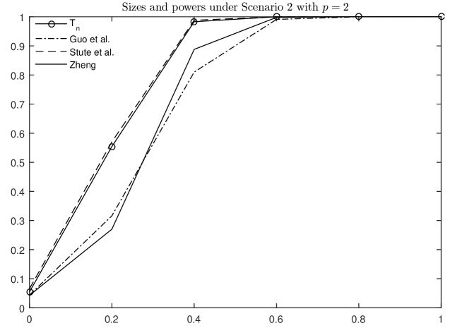
Figure 1: The empirical size and powers curves of $T_{n}$, $T^{GWZ}$, $T^{S}$ and $T^{Zh}$ in Scenario 2 $n=200$ with $p=2$ and $p=8$.

In this scenario, we test against a low-frequency alternative model. The parameters are $\beta_{1}=(\underbrace{1,\dots,1}_{p/2},0,\dots,0)^{\top}/\sqrt{p/2}$ and $\beta_{2}=(\underbrace{0,\dots,0}_{p/2},1,\dots,1)^{\top}/\sqrt{p/2}$. The sample size $n=200$ and $p=2,8$. $X$ and $\varepsilon$ follow the same distribution in Scenario 1, i.e. $X\sim N(0,I_{p})$ and $\varepsilon\sim N(0,1)$. We use $a=0.2,0.6,1$ under the alternative models. The plots of the power line is shown in Figure 1.

Figure 1 about here.

The results give us the following observations. When $p=2$, the global smoothing test $T^{S}$ works well and $T_{n}$ performs similarly or very slightly worse compared with $T^{S}$. Two local smoothing tests $T^{GWZ}$ and $T^{Zh}$ have inferior performance than $T^{S}$ and $T_{n}$. This again shows that $T_{n}$ has the advantage a global smoothing test should have. This justifies that low-frequency models are in favor of global smoothing tests. When $p=8$, $T^{S}$ is seriously affected by the dimension, the influence of the dimension $p$ to $T_{n}$ is limited.

In the first two scenarios, $X\sim N(0,I_{p})$ and thus the components of $X$ are uncorrelated from each other. Now we consider correlated case.

Scenario 3. Consider

$$Y=\beta^{\top}X+a\cdot\exp(-(\beta^{\top}X)^{2})+\varepsilon.$$

Two settings are considered: $X\sim N(0,\Sigma)$ where $\Sigma=(0.5^{|i-j|})_{p\times p}$. The error $\varepsilon\sim N(0,1)$. We test with dimension $p=2,4,8$, sample size $n=200$ and parameter $\beta=(1,1,\dots,1)^{\top}/\sqrt{p}$. Results are presented in Table 2.

Table 2 about here.

When $p=2$ and $p=4$, $T^{S}$, $T^{GWZ}$ and our test have similar powers while $T^{Zh}$ does not work well. When the dimension is raised up to $p=8$, $T^{GWZ}$ and $T_{n}$ become the winner. As $T^{GWZ}$ adopts the dimension reduction structure under the null in this setting, its good performance is understandable. $T_{n}$, however, requires no model structure information and performs similarly as $T^{GWZ}$.

The above three scenarios are all concerned with the linear model under the null hypothesis, therefore a nonlinear null model is used in the following scenario. Denote $X_{i}$ as the $i$th component of $X$.

Scenario 4. Consider

$$Y=\exp(c_{1}X_{1})+(c_{2}X_{2})^{3}+c_{3}\sin(\pi X_{3})+c_{4}|X_{4}|+c_{5}X_{5}\cdot X_{6}+a\cdot\cos(\beta^{\top}X)+\varepsilon$$

where $c_{1}=c_{2}=\dots=c_{5}=1/\sqrt{6}$ and $\beta=(0,1,1,0,\dots,0)^{\top}$.

This model does not have a dimension reduction structure under the null hypothesis and thus it not in favor of $T^{GWZ}$ that is designed for single index models. To make a comparison, we adopt its model adaptation idea by using the following test statistic as

$$nh^{\hat{q}/2}\cdot\frac{1}{n(n-1)}\sum_{i=1}^{n}\sum_{j\neq i}\hat{e}_{i}\hat{e}_{j}\frac{1}{h^{\hat{q}}}K(\frac{\hat{B}_{\hat{q}}^{\top}(x_{i}-x_{j})}{h}).$$

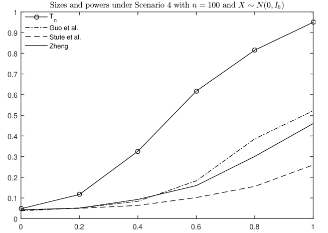
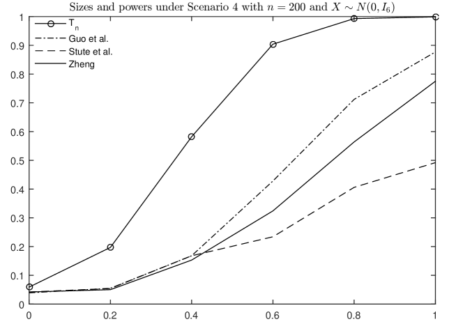
Figure 3: The empirical size and power curves of $T_{n}$, $T^{GWZ}$, $T^{S}$ and $T^{Zh}$ in Scenario 4 with $n=100,200$ and $X\sim N(0,I_{6})$.

Figure 3 about here.

The results in Figure 3 clearly suggest that the proposed test $T_{n}$ performs much better than the competitors no matter they are either local or global smoothing tests. This further confirms the advantages of the new method.

4.2 Real data analysis

We now analyze the Auto MPG data set that can be downloaded from the UCI Machine Learning Repository Lichman (2013). Quinlan (1993) firstly used the data set and recently Xia (2007) and Guo et al. (2016) as an illustration for their methods. A linear regression model was build in Quinlan (1993). Here we use the proposed test to check the adequacy of the linear model. The response variate $Y$ is mpg: miles per gallon. The first 6 attributes, noted from $X_{1}$ to $X_{6}$, includes running year of the model, acceleration time from still state to 60 miles per hour, car weight, horsepower, displacement of the engine and the number of cylinders. For the multi-valued independent variable origin, we introduce dummy variables as Guo et al. (2016) and Xia (2007) did. One of the new indicator variables $X_{7}=1$ if the car is from America; otherwise, $X_{7}=0$. Another dummy variable $X_{8}$ indicates whether the car is from Europe. The attributes are standardized one by one. The $p$-value is about $0$ and thus, the linear model is not suitable for this data set. The result is coincident with Guo et al. (2016).

5 Discussions

In this paper, we build a bridge between local smoothing test and global smoothing test and propose a test that is local smoothing-based is of the global smoothing nature. Therefore, the test benefits both advantages of these two types of testing procedures. The theoretical properties and empirical studies confirm this nice feature. The approach may be applicable to other types of data and testing problems. These are ongoing.

Appendix

Proofs of Lemma 2.2..

Recall the formula of $\hat{V}$, the integral can be computed as

$$\int_{R^{p}}\frac{1}{h}K\left(\frac{\alpha^{\top}(x_{i}-x_{j})}{h}\right)\mu(\alpha)d\alpha$$

$$= h^{-1}\int_{R^{p}}(2\pi)^{-1/2}\exp\left(-\frac{\alpha^{\top}(x_{i}-x_{j})(x_{i}-x_{j})^{\top}\alpha}{2h^{2}}\right)\cdot(2\pi)^{-p/2}\sigma_{\alpha}^{-p}\exp\left(-\frac{\alpha^{\top}\alpha}{2\sigma^{2}}\right)d\alpha$$

$$= h^{-1}(2\pi)^{-1/2}\sigma_{\alpha}^{-p}\int_{R^{p}}(2\pi)^{-p/2}\exp\left(-\frac{1}{2}\alpha^{\top}\left(\frac{(x_{i}-x_{j})(x_{i}-x_{j})^{\top}}{h^{2}}+\frac{1}{\sigma^{2}}I_{p}\right)\alpha\right)d\alpha.$$

Define $\Sigma_{ij}^{-1}=\frac{(x_{i}-x_{j})(x_{i}-x_{j})^{\top}}{h^{2}}+\frac{1}{\sigma^{2}}I_{p}$. Then the integral (Proofs of Lemma 2.2..) becomes

$$h^{-1}(2\pi)^{-1/2}\sigma^{-p}\int_{R^{p}}(2\pi)^{-p/2}\exp\left(-\frac{1}{2}\alpha^{\top}\Sigma_{ij}^{-1}\alpha\right)d\alpha$$ (5.2)

$$= h^{-1}(2\pi)^{-1/2}\sigma^{-p}|\Sigma_{ij}|^{1/2}\int_{R^{p}}(2\pi)^{-p/2}|\Sigma_{ij}|^{-1/2}\exp\left(-\frac{1}{2}\alpha^{\top}\Sigma_{ij}^{-1}\alpha\right)d\alpha$$

$$= h^{-1}(2\pi)^{-1/2}\sigma^{-p}|\Sigma_{ij}|^{1/2}.$$

Next we study the property of $\Sigma_{ij}$ to get $|\Sigma_{ij}|$. Let

$$A_{ij} = \frac{(x_{i}-x_{j})(x_{i}-x_{j})^{\top}}{h^{2}}.$$

The matrix $A_{ij}$ is symmetric and $rank(A_{ij})=1$. By some algebraic calculations, $A_{ij}$ has a nonzero eigenvalue $\frac{d_{ij}}{h^{2}}$ where $d_{ij}=\|x_{i}-x_{j}\|^{2}=(x_{i}-x_{j})^{\top}(x_{i}-x_{j})$. Therefore, it is well known that $\Sigma_{ij}^{-1}=A_{ij}+I_{p}/\sigma^{2}$ can be decomposed as

$$A\begin{pmatrix}\frac{d_{ij}}{h^{2}}+\frac{1}{\sigma^{2}}&&&\\ &\frac{1}{\sigma^{2}}&&\\ &&\ddots&\\ &&&\frac{1}{\sigma^{2}}.\end{pmatrix}A^{\top},$$

for some non-singular matrix $A$ where the elements on the diagonal of the matrix inside are the eigenvalues of $\Sigma_{ij}^{-1}$ and the determination is

$$|\Sigma_{ij}|=(\frac{d_{ij}}{h^{2}}+\frac{1}{\sigma^{2}})^{-1}(\sigma^{2})^{p-1}.$$ (5.3)

From (Proofs of Lemma 2.2..) – (5.3), the estimate in (2.2) can be written as

$$\hat{V} = \frac{1}{n(n-1)}\sum_{i=1}^{n}\sum_{j\neq i}\hat{e}_{i}\hat{e}_{j}h^{-1}(2\pi)^{-1/2}\sigma^{-p}(\frac{d_{ij}}{h^{2}}+\frac{1}{\sigma^{2}})^{-1/2}\sigma^{p-1}$$ (5.4)

$$= \frac{1}{\sqrt{2\pi}}\cdot\frac{1}{n(n-1)}\sum_{i=1}^{n}\sum_{j\neq i}\hat{e}_{i}\hat{e}_{j}\frac{1}{\sqrt{\sigma^{2}d_{ij}+h^{2}}}.$$

When $\sigma^{2}$ is chosen to be $h^{2}$, we have

$$\hat{V}=\frac{1}{h\sqrt{2\pi}}\cdot\frac{1}{n(n-1)}\sum_{i=1}^{n}\sum_{j\neq i}\hat{e}_{i}\hat{e}_{j}\frac{1}{\sqrt{d_{ij}+1}}.$$ (5.5)

∎

Designed Conditions

The following conditions are for the consistency and asymptotic normality of $\hat{\theta}_{n}$.

1. $\{(x_{i},y_{i})\}_{i=1,\dots,n}$ are i.i.d. random samples from $(X,Y)$ in $R^{p}\times R$ and $EY^{2}<\infty$.

2. The parameter $\Theta$ is compact and convex.

3. The regression function $g(x,\theta)$ is a Borel measurable real function on $R^{p}$ for each $\theta$ and is twice continuously differentiable with respect to $\theta$ for each $x$.

4. Let $\|\cdot\|$ represent the Euclidean norm.

   $$E(\sup_{\theta\in\Theta}g^{2}(X,\theta))<\infty,$$

   $$E(\sup_{\theta\in\Theta}\|\frac{\partial g(X,\theta)}{\partial\theta}\cdot\frac{\partial g(X,\theta)}{\partial\theta^{\top}}\|)<\infty,$$

   $$E(\sup_{\theta\in\Theta}\|(Y-g(X,\theta))^{2}\cdot\frac{\partial g(X,\theta)}{\partial\theta}\cdot\frac{\partial g(X,\theta)}{\partial\theta^{\top}}\|<\infty,$$

   $$E(\sup_{\theta\in\Theta}\|(Y-g(X,\theta))\cdot\frac{\partial^{2}g(X,\theta)}{\partial\theta\partial\theta^{\top}}\|)<\infty.$$

5. There exists a unique minimizer $\theta^{\ast}$ such that

   $$\theta^{\ast}=\arg\inf_{\theta\in R^{d}}E(Y-g(X,\theta))^{2}.$$

   Under the null hypothesis, $\theta^{\ast}$ is an interior point of $\Theta$.

6. The matrix $E(\frac{\partial g(X,\theta)}{\partial\theta}\cdot\frac{\partial g(X,\theta)}{\partial\theta^{\top}})$ is nonsingular.

The following lemma shows the asymptotic property of $\hat{\theta}_{n}$.

Lemma 5.1.

Suppose that the above conditions are satisfied, we have the following asymptotic properties. Denote $H_{\dot{g}}=E(\dot{g}(X,\theta^{\ast})\dot{g}(X,\theta^{\ast})^{\top})$ .

1. Under the null hypothesis, $\theta^{\ast}=\theta_{0}$ and

   $$\sqrt{n}(\hat{\theta}_{n}-\theta^{\ast})=H_{\dot{g}}^{-1}\frac{1}{\sqrt{n}}\sum_{i=1}^{n}\varepsilon_{i}\dot{g}(x_{i},\theta^{\ast})+o_{p}(1).$$

2. Under the local alternative models with $\delta_{n}\to 0$, $\theta^{\ast}=\theta_{0}$ and

   $$\sqrt{n}(\hat{\theta}_{n}-\theta^{\ast})=H_{\dot{g}}^{-1}\frac{1}{\sqrt{n}}\sum_{i=1}^{n}\varepsilon_{i}\dot{g}(x_{i},\theta^{\ast})+\sqrt{n}\delta_{n}\cdot H_{\dot{g}}^{-1}E(\ell\dot{g})+o_{p}(1).$$

3. Under the global alternative model with a fixed $\delta_{n}$, $\theta^{\ast}=\theta_{1}$ where

   $$\theta_{1}=\arg\min\limits_{\theta\in\Theta}E(g(X,\theta_{0})-g(X,\theta)+\delta_{n}\ell(X))^{2}$$

   and

   $$\hat{\theta}_{n}-\theta^{\ast} = O_{p}(\frac{1}{\sqrt{n}}).$$

Proofs of Lemma 5.1..

The least squares estimate of $\theta_{0}$ is the minimizer of the following function over all $\theta\in\Theta$ as

$$Q(\theta) = \frac{1}{n}\sum_{i=1}^{n}(y_{i}-g(x_{i},\theta))^{2},$$

$$\hat{\theta}_{n} = \arg\min\limits_{\theta\in\Theta}Q(\theta).$$

The first order derivative of $Q$ with respect to $\theta$ is

$$\dot{Q}(\theta) = -\frac{2}{n}\sum_{i=1}^{n}(y_{i}-g(x_{i},\theta))\dot{g}(x_{i},\theta)$$

where $\dot{g}=\partial g/\partial\theta$. The second order derivative of $Q$ with respect to $\theta$ is

$$\ddot{Q}(\theta) = \frac{2}{n}\sum_{i=1}^{n}\dot{g}(x_{i},\theta)g(x_{i},\theta)^{\top}-\frac{2}{n}\sum_{i=1}^{n}(y_{i}-g(x_{i},\theta))\ddot{g}(x_{i},\theta)$$

The least squares estimate $\hat{\theta}_{n}$ satisfies $\dot{Q}(\hat{\theta}_{n})=0$. Notice that $\frac{1}{n}\sum_{i=1}^{n}(y_{i}-g(x_{i},\theta))^{2}\overset{a.s.}{\to}E(Y-g(X,\theta))^{2}$ for all $\theta$, the estimator $\hat{\theta}_{n}\overset{a.s.}{\to}\theta^{\ast}$. Applying the Taylor expansion to $\dot{Q}(\hat{\theta}_{n})$ around $\theta^{\ast}$, we have

$$\dot{Q}(\hat{\theta}_{n})-\dot{Q}(\theta^{\ast}) = \ddot{Q}(\tilde{\theta})(\hat{\theta}_{n}-\theta^{\ast})$$

$$\hat{\theta}_{n}-\theta^{\ast} = \ddot{Q}(\tilde{\theta})^{-1}(\dot{Q}(\hat{\theta}_{n})-\dot{Q}(\theta^{\ast}))$$

$$= -\ddot{Q}(\tilde{\theta})^{-1}\dot{Q}(\theta^{\ast})$$

where $\tilde{\theta}$ is a mid-value between $\hat{\theta}_{n}$ and $\theta^{\ast}$. Since $\tilde{\theta}$ is close to $\theta^{\ast}$, it is easy to show that

$$\sqrt{n}(\hat{\theta}_{n}-\theta^{\ast}) = -E(\ddot{Q}(\theta^{\ast}))^{-1}\sqrt{n}\dot{Q}(\theta^{\ast})+o_{p}(1)$$

$$= 2E(\ddot{Q}(\theta^{\ast}))^{-1}\frac{1}{\sqrt{n}}\sum_{i}(y_{i}-g(x_{i},\theta^{\ast}))\dot{g}(x_{i},\theta^{\ast})+o_{p}(1).$$

Under the null hypothesis and the local alternatives with $\delta_{n}\to 0$,

$$\inf_{\theta\in\Theta}E(Y-g(X,\theta))^{2} = \inf_{\theta\in\Theta}E(g(X,\theta_{0})-g(X,\theta))^{2}+E(\varepsilon)^{2}.$$

thus $\theta^{\ast}=\theta_{0}$. Specifically, under the null hypothesis, $y_{i}-g(x_{i},\theta^{\ast})=\varepsilon_{i}$ and

$$E(\ddot{Q}(\theta^{\ast})) = 2E(\dot{g}(X,\theta^{\ast})\dot{g}(X,\theta^{\ast})^{\top})+2E(\varepsilon\ddot{g})$$

$$= 2H_{\dot{g}}$$

thus

$$\sqrt{n}(\hat{\theta}_{n}-\theta^{\ast}) = H_{\dot{g}}^{-1}\frac{1}{\sqrt{n}}\sum_{i=1}^{n}\varepsilon_{i}\dot{g}(x_{i},\theta^{\ast})+o_{p}(1).$$

Under the local alternative hypothesis, $y_{i}-g(x_{i},\theta^{\ast})=\varepsilon_{i}+\delta_{n}\ell(x_{i})$ and

$$E(\ddot{Q}(\theta^{\ast})) = 2E(\dot{g}(X,\theta^{\ast})\dot{g}(X,\theta^{\ast})^{\top})+2E(\varepsilon\ddot{g})+2\delta_{n}E(\ell\dot{g})$$

$$= 2H_{\dot{g}}+o_{p}(1).$$

Hence

$$\sqrt{n}(\hat{\theta}_{n}-\theta^{\ast}) = H_{\dot{g}}^{-1}\frac{1}{\sqrt{n}}\sum_{i=1}^{n}\varepsilon_{i}\dot{g}(x_{i},\theta^{\ast})+\sqrt{n}\delta_{n}\cdot H_{\dot{g}}^{-1}\frac{1}{n}\sum_{i=1}^{n}\ell(x_{i})\dot{g}(x_{i},\theta^{\ast})+o_{p}(1)$$

$$= H_{\dot{g}}^{-1}\frac{1}{\sqrt{n}}\sum_{i=1}^{n}\varepsilon_{i}\dot{g}(x_{i},\theta^{\ast})+\sqrt{n}\delta_{n}\cdot H_{\dot{g}}^{-1}E(\ell\dot{g})+o_{p}(1).$$

Under the global alternative with $\delta_{n}$ fixed,

$$\inf_{\theta\in\Theta}E(Y-g(X,\theta))^{2} = \inf_{\theta\in\Theta}E(g(X,\theta_{0})-g(X,\theta)+\delta_{n}\ell(X))^{2}+E(\varepsilon)^{2}.$$

The minimizer

$$\theta^{\ast}=\theta_{1}=\arg\inf_{\theta\in\Theta}E(Y-g(X,\theta))^{2}$$

is a value that is more likely to be different from $\theta_{0}$ under the null hypothesis. In this case,

$$E(\ddot{Q}(\theta^{\ast})) = 2H_{\dot{g}}-2E\{[g(X,\theta_{0})-g(X,\theta_{1})+\delta_{n}\ell(X)]\ddot{g}(X,\theta_{1})\}$$

$$\sqrt{n}(\hat{\theta}_{n}-\theta^{\ast}) = 2E(\ddot{Q}(\theta^{\ast}))^{-1}\frac{1}{\sqrt{n}}\sum_{i}(y_{i}-g(x_{i},\theta^{\ast}))\dot{g}(x_{i},\theta^{\ast})+o_{p}(1).$$

Notice that at the population level,

$$0=\frac{\partial E(Y-g(X,\theta))^{2}}{\partial\theta}|_{\theta=\theta^{\ast}}=-2E[(Y-g(X,\theta^{\ast}))\dot{g}(X,\theta^{\ast})].$$

Therefore under the global alternative hypothesis,

$$\sqrt{n}(\hat{\theta}_{n}-\theta^{\ast}) \overset{d}{\to} N(0,\Sigma_{1})$$

where $\Sigma_{1}=4E(\ddot{Q}(\theta^{\ast}))^{-1}E((Y-g(X,\theta^{\ast}))^{2}\dot{g}(X,\theta^{\ast})\dot{g}(X,\theta^{\ast})^{\top})E(\ddot{Q}(\theta^{\ast}))^{-1}$. ∎

Proofs of the theorems

Define $w_{ij}=\frac{1}{\sqrt{\lambda_{ij}+1}}$ which is symmetric about $x_{i}$ and $x_{j}$. The integrated statistic $V_{n}$ can be decomposed as:

$$V_{n} = \frac{1}{n(n-1)}\sum_{i=1}^{n}\sum_{j\neq i}\hat{e}_{i}\hat{e}_{j}w_{ij}$$ (5.6)

$$= \frac{1}{n(n-1)}\sum_{i=1}^{n}\sum_{j\neq i}e_{i}e_{j}w_{ij}-\frac{2}{n(n-1)}\sum_{i=1}^{n}\sum_{i\neq j}e_{i}(e_{j}-\hat{e}_{j})w_{ij}$$

$$+\frac{1}{n(n-1)}\sum_{i=1}^{n}\sum_{j\neq i}(e_{i}-\hat{e}_{i})(e_{j}-\hat{e}_{j})w_{ij}$$

$$=\mathrel{\mathop{\mathchar 58\relax}} V_{1}-2V_{2}+V_{3}.$$

Proofs of Theorem 3.1. .

Under the null hypothesis, $e=\varepsilon$,

$$V_{1} = \frac{1}{n(n-1)}\sum_{i=1}^{n}\sum_{j\neq i}\varepsilon_{i}\varepsilon_{j}w_{ij},$$

$$V_{2} = \frac{1}{n(n-1)}\sum_{i=1}^{n}\sum_{j\neq i}\varepsilon_{i}(\varepsilon_{j}-\hat{\varepsilon}_{j})w_{ij}$$

$$= \frac{1}{n(n-1)}\sum_{i=1}^{n}\sum_{j\neq i}\varepsilon_{i}\dot{g}_{j}^{\top}(\hat{\theta}_{n}-\theta_{0})w_{ij}+O_{p}(n^{-3/2})$$

$$= \frac{1}{n}\sum_{i=1}^{n}\varepsilon_{i}(\frac{1}{n-1}\sum_{j\neq i}\dot{g}_{j}w_{ij})^{\top}(\hat{\theta}_{n}-\theta_{0})+O_{p}(n^{-3/2})$$

$$= \frac{1}{n}\sum_{i=1}^{n}\varepsilon_{i}(\hat{\theta}_{n}-\theta_{0})^{\top}E_{1i}+O_{p}(n^{-3/2})$$

$$= \frac{1}{n^{2}}\sum_{i=1}^{n}\sum_{j=1}^{n}\varepsilon_{i}\varepsilon_{j}\dot{g}_{j}^{\top}H_{\dot{g}}^{-1}E_{1i}+O_{p}(n^{-3/2})$$

$$= \frac{n-1}{n}\cdot\frac{1}{n(n-1)}\sum_{i=1}^{n}\sum_{j\neq i}^{n}\varepsilon_{i}\varepsilon_{j}\dot{g}_{j}^{\top}H_{\dot{g}}^{-1}E_{1i}+\frac{1}{n^{2}}\sum_{i=1}^{n}\varepsilon_{i}^{2}\dot{g}_{i}^{\top}H_{\dot{g}}^{-1}E_{1i}+O_{p}(n^{-3/2}).$$

Define

$$V_{2}^{0} = \frac{1}{n(n-1)}\sum_{i=1}^{n}\sum_{j\neq i}\varepsilon_{i}\varepsilon_{j}\dot{g}_{j}^{\top}H_{\dot{g}}^{-1}E_{1i}=O_{p}(\frac{1}{n}),~{}~{}~{}E_{1i}=E_{j}(\dot{g}_{j}w_{ij}),$$

$$\mu_{v_{2}} = E(\varepsilon_{i}^{2}\dot{g}_{i}^{\top}H_{\dot{g}}^{-1}E_{1i})=E(\sigma_{i}^{2}\dot{g}_{i}^{\top}H_{\dot{g}}^{-1}E_{1i}),~{}~{}~{}\sigma_{i}^{2}=E(\varepsilon^{2}|x_{i}).$$

Then

$$nV_{2}=nV_{2}^{0}+\mu_{v_{2}}+O_{p}(n^{-1/2})$$ (5.7)

For $V_{3}$, we have a similar decomposition as,

$$V_{3} = \frac{1}{n(n-1)}\sum_{i=1}^{n}\sum_{j\neq i}(\varepsilon_{i}-\hat{\varepsilon}_{i})(\varepsilon_{j}-\hat{\varepsilon}_{j})w_{ij}$$

$$= \frac{1}{n(n-1)}\sum_{i=1}^{n}\sum_{j\neq i}(\hat{\theta}_{n}-\theta_{0})^{\top}\dot{g}_{i}\dot{g}_{j}^{\top}(\hat{\theta}_{n}-\theta_{0})w_{ij}+O_{p}(n^{-3/2})$$

$$= (\hat{\theta}_{n}-\theta_{0})^{\top}\cdot\frac{1}{n(n-1)}\sum_{i=1}^{n}\sum_{j\neq i}\dot{g}_{i}\dot{g}_{j}^{\top}w_{ij}\cdot(\hat{\theta}_{n}-\theta_{0})+O_{p}(n^{-3/2})$$

$$= \frac{1}{n^{2}}\sum_{i=1}^{n}\sum_{j=1}^{n}\varepsilon_{i}\varepsilon_{j}\dot{g}_{i}^{\top}H_{\dot{g}}^{-1}E(\dot{g}_{k}E_{1k}^{\top})H_{\dot{g}}^{-1}\dot{g}_{j}+O_{p}(n^{-3/2})$$

$$= \frac{1}{n^{2}}\sum_{i=1}^{n}\sum_{j\neq i}^{n}\varepsilon_{i}\varepsilon_{j}\dot{g}_{i}^{\top}H_{\dot{g}}^{-1}E(\dot{g}_{k}E_{1k}^{\top})H_{\dot{g}}^{-1}\dot{g}_{j}+\frac{1}{n^{2}}\sum_{i=1}^{n}\varepsilon_{i}^{2}\dot{g}_{i}^{\top}H_{\dot{g}}^{-1}E(\dot{g}_{k}E_{1k}^{\top})H_{\dot{g}}^{-1}\dot{g}_{i}+O_{p}(n^{-3/2}).$$

Define

$$V_{3}^{0} = \frac{1}{n(n-1)}\sum_{i=1}^{n}\sum_{j\neq i}\varepsilon_{i}\varepsilon_{j}\dot{g}_{i}^{\top}H_{\dot{g}}^{-1}E(\dot{g}_{k}E_{1k}^{\top})H_{\dot{g}}^{-1}\dot{g}_{j}=O_{p}(\frac{1}{n}),$$

$$\mu_{v_{3}} = E(\varepsilon^{2}_{i}\dot{g}_{i}^{\top}H_{\dot{g}}^{-1}E(\dot{g}_{k}E_{1k}^{\top})H_{\dot{g}}^{-1}\dot{g}_{i})=E(\sigma^{2}_{i}\dot{g}_{k}^{\top}H_{\dot{g}}^{-1}\dot{g}_{i}\dot{g}_{i}^{\top}H_{\dot{g}}^{-1}E_{1k}).$$

Then

$$nV_{3}=nV_{3}^{0}+\mu_{v_{3}}+O_{p}(n^{-1/2}).$$ (5.8)

If $\sigma_{\varepsilon}^{2}\equiv E(\varepsilon^{2}|X)$, then

$$\mu_{v_{3}}=\sigma_{\varepsilon}^{2}E(\dot{g}_{i}^{\top}H_{\dot{g}}^{-1}E_{1i})=\mu_{v_{2}}.$$

Then from (5.6) to (5.8) we can see $nV_{n}$ has the same asymptotic behavior as $nV_{n}^{0}+\mu_{0}$, i.e.

$$nV_{n}=nV_{n}^{0}+\mu_{0}+o_{p}(1)$$ (5.9)

where $V_{n}^{0}=V_{1}-2V_{2}^{0}+V_{3}^{0}$ and $\mu_{0}=\mu_{v_{3}}-2\mu_{v_{2}}$.

Denote

$$\tilde{w}_{ij}=w_{ij}-2\dot{g}_{j}^{\top}H_{\dot{g}}^{-1}E_{1i}+\dot{g}_{i}^{\top}H_{\dot{g}}^{-1}E(\dot{g}_{k}E_{1k}^{\top})H_{\dot{g}}^{-1}\dot{g}_{j},$$

then

$$V_{n}^{0}=\frac{1}{n(n-1)}\sum_{i=1}^{n}\sum_{j\neq i}\varepsilon_{i}\varepsilon_{j}\tilde{w}_{ij}.$$

$V_{n}^{0}$ can be represented by a U-statistic. Let

$$h(x_{i},x_{j})=\frac{1}{2}\left(\tilde{w}_{ij}+\tilde{w}_{ji}\right),$$

then $V_{n}^{0}$ has the same limiting distribution as

$$U_{n}=\frac{1}{n(n-1)}\sum_{i=1}^{n}\sum_{j\neq i}\varepsilon_{i}\varepsilon_{j}h(x_{i},x_{j}).$$ (5.10)

This is a degenerate U-statistic and details of its asymptotic distribution can be found in chapter 5, Serfling (1980). Here we simply show the results. Let $\lambda_{1},\lambda_{2},\dots$ be the corresponding eigenvalues to the distinct solutions $s_{1},s_{2},\dots$ satisfying that

$$\int_{-\infty}^{\infty}h(x_{i},x_{j})s(x_{j})dF(x_{j})=\lambda s(x_{i})$$

where $F(\cdot)$ is the cumulative distribution function of $X$. Based on (5.9) and (5.10), the limiting null distribution of our test statistic is

$$T_{n}\overset{\Delta}{=}nV_{n}\overset{d}{\to}\sum_{i=1}^{\infty}\lambda_{i}(Z_{i}^{2}-1)+\mu_{0}$$

where $Z_{1},Z_{2},\dots$ are independent standard normal random variables. ∎

Proofs of Theorem 3.2. .

Under the alternative hypothesis,

$$Y=g(X,\theta)+\delta_{n}\ell(X)+\varepsilon.$$

therefore $e_{i}=\delta_{n}\ell(x_{i})+\varepsilon_{i}$.

Firstly, consider the global alternative hypothesis where $\delta_{n}$ is some constant. $V_{n}$ can be decomposed as

$$V_{n} = \frac{1}{n(n-1)}\sum_{i=1}^{n}\sum_{j\neq i}\hat{e}_{i}\hat{e}_{j}w_{ij}$$ (5.11)

$$= \frac{1}{n(n-1)}\sum_{i=1}^{n}\sum_{j\neq i}e_{i}e_{j}w_{ij}-\frac{2}{n(n-1)}\sum_{i=1}^{n}\sum_{i\neq j}e_{i}(e_{j}-\hat{e}_{j})w_{ij}$$

$$+\frac{1}{n(n-1)}\sum_{i=1}^{n}\sum_{j\neq i}(e_{i}-\hat{e}_{i})(e_{j}-\hat{e}_{j})w_{ij}$$

$$= V_{1}-2V_{2}+V_{3}.$$

For the second term,

$$V_{2} = \frac{1}{n(n-1)}\sum_{i=1}^{n}\sum_{j\neq i}e_{i}(e_{j}-\hat{e}_{j})w_{ij}$$ (5.12)

$$= \frac{1}{n(n-1)}\sum_{i=1}^{n}\sum_{j\neq i}e_{i}\dot{g}_{j}^{\top}(\hat{\theta}_{n}-\theta_{0})w_{ij}+o_{p}(V_{2}^{\ast}),$$

$$V_{2}^{\ast} = \frac{1}{n(n-1)}\sum_{i=1}^{n}\sum_{j\neq i}e_{i}\dot{g}_{j}^{\top}(\hat{\theta}_{n}-\theta_{0})w_{ij}$$ (5.13)

$$= \frac{1}{n(n-1)}\sum_{i=1}^{n}\sum_{j\neq i}e_{i}\dot{g}_{j}^{\top}w_{ij}\cdot o_{p}(1)$$

$$= E(\ell_{i}\dot{g}_{j}^{\top}w_{ij})\cdot o_{p}(1)$$

$$= o_{p}(1).$$

For the third term,

$$V_{3} = \frac{1}{n(n-1)}\sum_{i=1}^{n}\sum_{j\neq i}(e_{i}-\hat{e}_{i})(e_{j}-\hat{e}_{j})w_{ij}$$ (5.14)

$$= (\hat{\theta}_{n}-\theta_{0})^{\top}\cdot\frac{1}{n(n-1)}\sum_{i=1}^{n}\sum_{j\neq i}\dot{g}_{i}\dot{g}_{j}^{\top}w_{ij}\cdot(\hat{\theta}_{n}-\theta_{0})+o_{p}(V_{3}^{\ast}),$$

$$V_{3}^{\ast} = (\hat{\theta}_{n}-\theta_{0})^{\top}\cdot\frac{1}{n(n-1)}\sum_{i=1}^{n}\sum_{j\neq i}\dot{g}_{i}\dot{g}_{j}^{\top}w_{ij}\cdot(\hat{\theta}_{n}-\theta_{0})$$ (5.15)

$$= o_{p}(1)\cdot E(\dot{g}_{i}\dot{g}_{j}^{\top}w_{ij})\cdot o_{p}(1)+o_{p}(1)$$

$$= o_{p}(1).$$

Hence from (5.11) to (5.15), we have $V_{n}=V_{1}+o_{p}(1)$ . When $\delta_{n}$ is fixed,

$$V_{1} \overset{p}{\to} \mu_{1}=E(e_{i}e_{j}w_{ij})=E(\delta_{n}^{2}\ell(x_{i})\ell(x_{j})w(x_{i},x_{j})).$$

Therefore under the global alternative hypothesis,

$$T_{n}/n\overset{p}{\to}\mu_{1}.$$

Next, we consider the local alternative where $\delta_{n}\to 0$. Similar with the proof under the null distribution, we have

$$V_{n} = \frac{1}{n(n-1)}\sum_{i=1}^{n}\sum_{j\neq i}\hat{e}_{i}\hat{e}_{j}w_{ij}$$

$$= \frac{1}{n(n-1)}\sum_{i=1}^{n}\sum_{j\neq i}e_{i}e_{j}\tilde{w}_{ij}+\frac{1}{n}\mu_{0}+o_{p}(\frac{1}{n})$$

$$= \frac{1}{n(n-1)}\sum_{i=1}^{n}\sum_{j\neq i}\varepsilon_{i}\varepsilon_{j}\tilde{w}_{ij}+\delta_{n}\cdot\frac{1}{n(n-1)}\sum_{i=1}^{n}\sum_{j\neq i}[\ell_{i}\varepsilon_{j}+\varepsilon_{i}\ell_{j}]\tilde{w}_{ij}$$

$$+\delta_{n}^{2}\cdot\frac{1}{n(n-1)}\sum_{i=1}^{n}\sum_{j\neq i}\ell_{i}\ell_{j}\tilde{w}_{ij}+\frac{1}{n}\mu_{0}+o_{p}(\frac{1}{n})$$

$$= \frac{1}{n(n-1)}\sum_{i=1}^{n}\sum_{j\neq i}\varepsilon_{i}\varepsilon_{j}\tilde{w}_{ij}+\delta_{n}\cdot\frac{1}{n(n-1)}\sum_{i=1}^{n}\sum_{j\neq i}\varepsilon_{i}\ell_{j}(\tilde{w}_{ij}+\tilde{w}_{ji})$$

$$+\delta_{n}^{2}\cdot\frac{1}{n(n-1)}\sum_{i=1}^{n}\sum_{j\neq i}\ell_{i}\ell_{j}\tilde{w}_{ij}+\frac{1}{n}\mu_{0}+o_{p}(\frac{1}{n})$$

$$= \frac{1}{n(n-1)}\sum_{i=1}^{n}\sum_{j\neq i}\varepsilon_{i}[\varepsilon_{j}\tilde{w}_{ij}+\delta_{n}\ell_{j}(\tilde{w}_{ij}+\tilde{w}_{ji})]$$

$$+\delta_{n}^{2}\cdot\frac{1}{n(n-1)}\sum_{i=1}^{n}\sum_{j\neq i}\ell_{i}\ell_{j}\tilde{w}_{ij}+\frac{1}{n}\mu_{0}+o_{p}(\frac{1}{n}).$$

Define $M_{i}=E\left(\ell_{j}(\tilde{w}_{ij}+\tilde{w}_{ji})|x_{i}\right)$ and $\Delta_{\mu}=E(\ell_{i}\ell_{j}\tilde{w}_{ij})$. We have

$$E[\varepsilon_{j}\tilde{w}_{ij}+\delta_{n}\ell_{j}(\tilde{w}_{ij}+\tilde{w}_{ji})|x_{i}]=\delta_{n}E[\ell_{j}(\tilde{w}_{ij}+\tilde{w}_{ji})|x_{i}]=\delta_{n}M_{i}$$

and our test statistic

$$T_{n} = nV_{n}=\sqrt{n}\delta_{n}\cdot\frac{1}{\sqrt{n}}\sum_{i=1}^{n}\varepsilon_{i}M_{i}+n\delta_{n}^{2}\cdot\Delta_{\mu}+\mu_{0}+o_{p}(1).$$ (5.16)

From the expression in (5.16), the asymptotic behavior of $T_{n}$ can obtained. when $\delta_{n}=n^{-1/2}$, $T_{n}\overset{d}{\to}N(\mu_{1n},\Sigma)$ where $\mu_{1n}=\Delta_{\mu}+\mu_{0}$ and $\Sigma=Var(\varepsilon_{i}M_{i})$. When $\delta_{n}\to 0$ and $\sqrt{n}\delta_{n}\to\infty$ , $T_{n}/(n\delta_{n}^{2})\overset{p}{\to}\Delta_{\mu}$. ∎

Table 1: Empirical sizes and powers of $T_{n}$, $T^{GWZ}$, $T^{S}$ and $T^{Zh}$ for Scenario 1 with $X\sim N(0,I_{p})$, $\varepsilon\sim N(0,1)$ and $n=200$.

p=2	$T_{n}$	$T^{GWZ}$	$T^{S}$	$T^{Zh}$
a = 0.0	0.0570	0.054	0.066	0.043
0.2	0.3790	0.403	0.372	0.211
0.6	0.9950	1.000	0.998	0.991
1.0	0.9990	1.000	1.000	1.000
p=4	$T_{n}$	$T^{GWZ}$	$T^{S}$	$T^{Zh}$
a = 0.0	0.0480	0.050	0.044	0.042
0.2	0.3510	0.384	0.200	0.100
0.6	0.9620	0.999	0.936	0.684
1.0	0.9860	1.000	1.000	0.997
p=8	$T_{n}$	$T^{GWZ}$	$T^{S}$	$T^{Zh}$
a = 0.0	0.0610	0.050	0.028	0.036
0.2	0.3400	0.372	0.052	0.047
0.6	0.9290	1.000	0.104	0.371
1.0	0.9650	1.000	0.202	0.847

Table 2: Empirical sizes and powers of $T_{n}$, $T^{GWZ}$, $T^{S}$ and $T^{Zh}$ for Scenario 3 with $X\sim N(0,\Sigma)$ and $n=200$.

p=2	$T_{n}$	$T^{GWZ}$	$T^{S}$	$T^{Zh}$
a = 0.0	0.056	0.046	0.042	0.0465
0.2	0.339	0.274	0.32	0.1675
0.6	0.995	0.995	0.996	0.959
1.0	1	1.000	1	1
p=4	$T_{n}$	$T^{GWZ}$	$T^{S}$	$T^{Zh}$
a = 0.0	0.061	0.0465	0.058	0.047
0.2	0.266	0.213	0.192	0.0805
0.6	0.982	0.9795	0.92	0.5385
1.0	1	1	1	0.966
p=8	$T_{n}$	$T^{GWZ}$	$T^{S}$	$T^{Zh}$
a = 0.0	0.044	0.052	0.046	0.0365
0.2	0.243	0.211	0.1	0.054
0.6	0.944	0.9595	0.482	0.2875
1.0	1	1	0.85	0.743

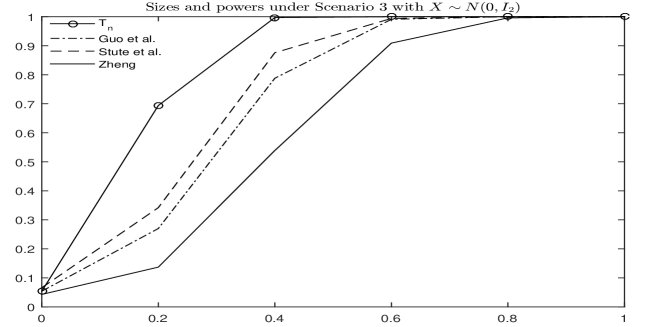
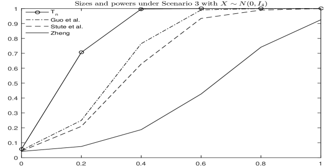
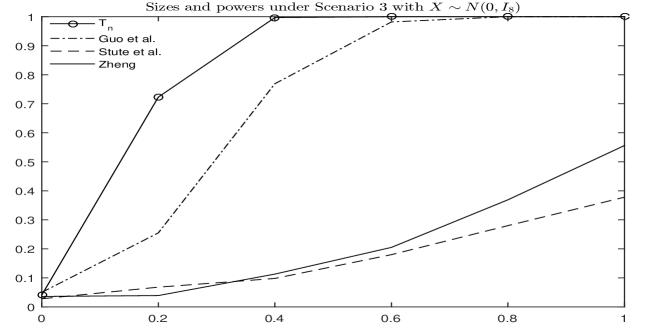
Figure 2: The empirical size and powers curves of $T_{n}$, $T^{GWZ}$, $T^{S}$ and $T^{Zh}$ in Scenario 3 $n=200$ with $X\sim N(0,I_{p})$.

References

- (1)
- An and Zhu (1992) An, H. and Zhu, L. (1992). A testing approach for nonlinearity in regression models, Journal of Mathematics 4: 004.
- Bierens (1982) Bierens, H. J. (1982). Consistent model specification tests, Journal of Econometrics 20(1): 105–134.
- Bierens (1990) Bierens, H. J. (1990). A consistent conditional moment test of functional form, Econometrica: Journal of the Econometric Society pp. 1443–1458.
- Delgado and Escanciano (2017) Delgado, M. A. and Escanciano, J. C. (2017). On the asymptotic efficiency of directional models checks for regression, Included in a book dedicated to Winfried Stute on the occasion of his 70th birthday, Springer International Publishing, in press.
- Escanciano (2006) Escanciano, J. C. (2006). A consistent diagnostic test for regression models using projections, Econometric Theory 22(6): 1030–1051.
- Friedman and Stuetzle (1981) Friedman, J. H. and Stuetzle, W. (1981). Projection pursuit regression, Journal of the American statistical Association 76(376): 817–823.
- Guo et al. (2016) Guo, X., Wang, T. and Zhu, L. (2016). Model checking for parametric single-index models: a dimension reduction model-adaptive approach, Journal of the Royal Statistical Society: Series B (Statistical Methodology) 78(5): 1013–1035.
- Guo and Zhu (2017) Guo, X. and Zhu, L. (2017). A review on dimension reduction-based tests for regressions, Included in a book dedicated to Winfried Stute on the occasion of his 70th birthday, Springer International Publishing, in press.
- Huber (1985) Huber, P. J. (1985). Projection pursuit, The annals of Statistics pp. 435–475.
- Lavergne and Patilea (2008) Lavergne, P. and Patilea, V. (2008). Breaking the curse of dimensionality in nonparametric testing, Journal of Econometrics 143(1): 103–122.
- Lavergne and Patilea (2012) Lavergne, P. and Patilea, V. (2012). One for all and all for one: regression checks with many regressors, Journal of business & economic statistics 30(1): 41–52.
-
Lichman (2013)
Lichman, M. (2013).
UCI machine learning repository.
http://archive.ics.uci.edu/ml - Quinlan (1993) Quinlan, J. R. (1993). Combining instance-based and model-based learning, Proceedings of the Tenth International Conference on Machine Learning, pp. 236–243.
-
Stute (1997)
Stute, W. (1997).
Nonparametric model checks for regression, Ann. Statist. 25(2): 613–641.
https://doi.org/10.1214/aos/1031833666 - Stute, Manteiga and Quindimil (1998) Stute, W., Manteiga, W. G. and Quindimil, M. P. (1998). Bootstrap approximations in model checks for regression, Journal of the American Statistical Association 93(441): 141–149.
-
Stute, Thies and Zhu (1998)
Stute, W., Thies, S. and Zhu, L. (1998).
Model checks for regression: an innovation process approach, Ann. Statist. 26(5): 1916–1934.
https://doi.org/10.1214/aos/1024691363 - Stute et al. (2008) Stute, W., Xu, W. and Zhu, L. (2008). Model diagnosis for parametric regression in high-dimensional spaces, Biometrika 95(2): 451–467.
- Stute and Zhu (2002) Stute, W. and Zhu, L. (2002). Model checks for generalized linear models, Scandinavian Journal of Statistics 29(3): 535–545.
- Tan et al. (2016) Tan, F., Zhu, X. and Zhu, L. (2016). A projection-based adaptive-to-model test for regressions, arXiv preprint arXiv:1604.01874 .
- White (1981) White, H. (1981). Consequences and detection of misspecified nonlinear regression models, Journal of the American Statistical Association 76(374): 419–433.
- Xia (2007) Xia, Y. (2007). A constructive approach to the estimation of dimension reduction directions, The Annals of Statistics pp. 2654–2690.
- Zheng (1996) Zheng, J. X. (1996). A consistent test of functional form via nonparametric estimation techniques, Journal of Econometrics 75(2): 263–289.
- Zhu (2003) Zhu, L. (2003). Model checking of dimension-reduction type for regression, Statistica Sinica pp. 283–296.
- Zhu and Li (1998) Zhu, L. and Li, R. (1998). Dimension-reduction type test for linearity of a stochastic regression model, Acta Mathematicae Applicatae Sinica (English Series) 14(2): 165–175.