Robust Maximum Likelihood Estimation of Sparse Vector Error Correction Model

Abstract

In econometrics and finance, the vector error correction model (VECM) is an important time series model for cointegration analysis, which is used to estimate the long-run equilibrium variable relationships. The traditional analysis and estimation methodologies assume the underlying Gaussian distribution but, in practice, heavy-tailed data and outliers can lead to the inapplicability of these methods. In this paper, we propose a robust model estimation method based on the Cauchy distribution to tackle this issue. In addition, sparse cointegration relations are considered to realize feature selection and dimension reduction. An efficient algorithm based on the majorization-minimization (MM) method is applied to solve the proposed nonconvex problem. The performance of this algorithm is shown through numerical simulations.

Index Terms—  cointegration analysis, robust statistics, heavy-tails, outliers, group sparsity.

1 Introduction

The vector error correction model (VECM) [1] is very important in cointegration analysis to estimate and test for the long-run cointegrated equilibriums. It is widely used in time series modeling for financial returns and macroeconomic variables. In [2, 3], Engle and Granger first proposed the concept of “cointegration” to describe the linear stationary relationships in the nonstationary time series. Later, Johansen studied the statistical estimation and inference problem in time series cointegration modeling [4, 5, 6]. A VECM for $\mathbf{y}_{t}\in\mathbb{R}^{K}$ is given as follows:

$$\begin{array}[]{c}\Delta\mathbf{y}_{t}=\boldsymbol{\nu}+\boldsymbol{\Pi}\mathbf{y}_{t-1}+\sum_{i=1}^{p-1}\boldsymbol{\Gamma}_{i}\Delta\mathbf{y}_{t-i}+\boldsymbol{\varepsilon}_{t},\end{array}$$ (1)

where $\Delta$ is the first difference operator, i.e., $\Delta\mathbf{y}_{t}=\mathbf{y}_{t}-\mathbf{y}_{t-1}$, $\boldsymbol{\nu}$ denotes the drift, $\boldsymbol{\Pi}$ determines the long-run equilibriums, $\boldsymbol{\Gamma}_{i}$ ($i=1,\ldots,p-1$) contains the short-run effects, and $\boldsymbol{\varepsilon}_{t}$ is the innovation with mean $\mathbf{0}$ and covariance $\boldsymbol{\Sigma}$. Matrix $\boldsymbol{\Pi}$ has a reduced cointegration rank $r$, i.e., $\mathrm{rank}\left(\boldsymbol{\Pi}\right)=r<K$, and it can be written as $\boldsymbol{\Pi}=\boldsymbol{\alpha}\boldsymbol{\beta}^{T}$ ($\boldsymbol{\alpha},\boldsymbol{\beta}\in\mathbb{R}^{K\times r}$). Accordingly, $\mathbf{y}_{t}$ is said to be cointegrated with rank $r$, and $\boldsymbol{\beta}^{T}\mathbf{y}_{t}$ gives the long-run stationary time series defined by the cointegration matrix $\boldsymbol{\beta}$. Such long-run equilibriums are often implied by economic theory and can be used for statistical arbitrage [7].

It is well-known that financial returns and macroeconomic variables exhibit heavy-tails and are often associated with outliers due to external factors, like political and regulatory changes, as well as data corruption, like faulty observations and wrongly processed data [8]. These stylized features contradict the popular Gaussian noise assumption typically made in the theoretical analysis and estimation procedures with adverse effects in the estimated models. Cointegration analysis is particularly sensitive to these issues. Papers [9, 10, 11] discussed the properties of the Dickey-Fuller test and the Johansen test in the presence of outliers. Lucas studied such issues both from a theoretical and an empirical point of view [12, 13, 14]. To deal with the heavy-tails and outliers in time series modeling, simple and effective estimation methods are needed. In [15], the pseudo maximum likelihood estimators were introduced for VECM. In this paper, based on [15], we formulate the estimation problem based on the log-likelihood function of the Cauchy distribution as a conservative representative of the heavy-tailed distributions to better fit the heavy-tails and dampen the influence of outliers.

Sparse optimization [16] has become the focus of much research interest as a way to realize feature selection and dimension reduction (e.g., lasso [17]). In [18], element-wise sparsity was imposed on $\boldsymbol{\beta}$ in VECM modeling. As indicated by [19, 20], to realize the feature selection purpose, group sparsity is better since it can simultaneously reduce the same variable in all cointegration relations and naturally keep the geometry of the low-rank parameter space. In this paper, instead of imposing the group sparsity on $\boldsymbol{\beta}$, we equivalently put group sparsity on $\boldsymbol{\Pi}$ and add a rank constraint for it, which can realize the same target without the ahead factorization $\boldsymbol{\Pi}=\boldsymbol{\alpha}\boldsymbol{\beta}^{T}$. For sparsity pursuing, i.e., approximating the $\ell_{0}$-“norm”, rather than the popular $\ell_{1}$-norm, we use a nonconvex Geman-type function [21] which has a better approximation power. A smoothed counterpart is also firstly proposed to reduce the “singularity issue” in optimization, based on which the group sparsity regularizer of $\boldsymbol{\beta}$ is attained.

Robust estimation is somewhat underrated in financial applications due to the complex computations that are time and resource intensive. By considering the robust loss and the regularizer, a nonconvex optimization problem is finally formulated. The expectation-maximization (EM) is usually used to solve the robust losses (e.g., [22]). However, EM cannot be applied for our formulation. To deal with it, an efficient algorithm based on the majorization-minimization (MM) method is proposed with estimation performance numerically shown.

2 Robust Estimation of Sparse VECM

Suppose a sample path $\left\{\mathbf{y}_{t}\right\}_{t=1}^{N}$ ($N>K$) and the needed pre-sample values are available, then the VECM (1) can be written into a matrix form as follows:

$$\Delta\mathbf{Y} =\boldsymbol{\Pi}\mathbf{Y}_{-1}+\boldsymbol{\Gamma}\Delta\mathbf{X}+\mathbf{E},$$ (2)

where $\boldsymbol{\Gamma}=\left[\boldsymbol{\Gamma}_{1},\ldots,\boldsymbol{\Gamma}_{p-1},\boldsymbol{\nu}\right]$, $\Delta\mathbf{Y}=\left[\Delta\mathbf{y}_{1},\ldots,\Delta\mathbf{y}_{N}\right]$, $\mathbf{Y}_{-1}=\left[\mathbf{y}_{0},\ldots,\mathbf{y}_{N-1}\right]$, $\Delta\mathbf{X}=\left[\Delta\mathbf{x}_{1},\ldots,\Delta\mathbf{x}_{N}\right]$ with $\Delta\mathbf{x}_{t}=\left[\begin{array}[]{c}\Delta\mathbf{y}_{t-1}^{T},\ldots,\Delta\mathbf{y}_{t-p+1}^{T},1\end{array}\right]^{T}$, and $\mathbf{E}=\left[\boldsymbol{\varepsilon}_{1},\ldots,\boldsymbol{\varepsilon}_{N}\right]$.

2.1 Robustness Pursued by Cauchy Log-likelihood Loss

The robustness is pursued by a multivariate Cauchy distribution. Assume the innovations $\boldsymbol{\varepsilon}_{t}$’s in (1) follow Cauchy distribution, i.e., $\boldsymbol{\varepsilon}_{t}\sim\mathrm{Cauchy}\left(\boldsymbol{0},\boldsymbol{\Sigma}\right)$ with $\boldsymbol{\Sigma}\in\mathbb{S}_{++}^{K}$, then the probability density function is given by

$$g_{\boldsymbol{\theta}}\left(\boldsymbol{\varepsilon}_{t}\right)=\frac{\Gamma\left(\frac{1+K}{2}\right)}{\Gamma\left(\frac{1}{2}\right)\left(\nu\pi\right)^{\frac{K}{2}}}\left[\det\left(\boldsymbol{\Sigma}\right)\right]^{-\frac{1}{2}}\left(1+\boldsymbol{\varepsilon}_{t}^{T}\boldsymbol{\Sigma}^{-1}\boldsymbol{\varepsilon}_{t}\right)^{-\frac{1+K}{2}}.$$

The negative log-likelihood loss function of the Cauchy distribution for $N$ samples from (1) is written as follows:

$$\begin{array}[]{rl}&L\left(\boldsymbol{\theta}\right)=\frac{N}{2}\log\det\left(\boldsymbol{\Sigma}\right)+\frac{1+K}{2}\sum_{i=1}^{N}\log\Bigl{(}1+\\ &\quad\quad\quad\left\|\boldsymbol{\Sigma}^{-\frac{1}{2}}\left(\Delta\mathbf{y}_{i}-\boldsymbol{\Pi}\mathbf{y}_{i-1}-\boldsymbol{\Gamma}\Delta\mathbf{x}_{i-1}\right)\right\|_{2}^{2}\Bigr{)},\end{array}$$ (3)

where the constants are dropped and $\boldsymbol{\theta}\triangleq\left\{\boldsymbol{\Pi}\left(\boldsymbol{\alpha},\boldsymbol{\beta}\right),\boldsymbol{\Gamma},\boldsymbol{\Sigma}\right\}$.

2.2 Group Sparsity Pursued by Nonconvex Regularizer

For a vector $\mathbf{x}\in\mathbb{R}^{K}$, the sparsity level is usually measured by the $\ell_{0}$-“norm” (or $\mathrm{sgn}\left(\left|x\right|\right)$) as $\left\|\mathbf{x}\right\|_{0}=\sum_{i=1}^{K}\mathrm{sgn}\left(\left|x_{i}\right|\right)=k$, where $k$ is the number of nonzero entries in $\mathbf{x}$. Generally, applying the $\ell_{0}$-“norm” to different groups of variables can enforce group sparsity in the solutions. The $\ell_{0}$-“norm” is not convex and not continuous, which makes it computationally difficult and leads to intractable NP-hard problems. So, $\ell_{1}$-norm as the tightest convex relaxation is usually used to approximate the $\ell_{0}$-“norm” in practice, which is easier for optimization and still favors sparse solutions.

Tighter nonconvex sparsity-inducing functions can lead to better performance [16]. In this paper, to better pursue the sparsity and to remove the “singularity issue”, i.e., when using nonsmooth functions, the variable may get stuck at a nonsmooth point [23], a smooth nonconvex function based on the rational (Geman) function in [21] is used given as follows:

$$\begin{array}[]{l}\mathrm{rat}_{p}^{\epsilon}\left(x\right)=\begin{cases}\frac{px^{2}}{2\epsilon\left(p+\epsilon\right)^{2}},&\left|x\right|\leq\epsilon\\ \frac{\left|x\right|}{p+\left|x\right|}-\frac{2\epsilon^{2}+p\epsilon}{2\left(p+\epsilon\right)^{2}},&\left|x\right|>\epsilon\end{cases}.\end{array}$$

In order to attain feature selection in VECM, i.e., sparse cointegration relations, according to [19, 20], we can impose the row-wise group sparsity on matrix $\boldsymbol{\beta}$. In fact, due to $\boldsymbol{\Pi}=\boldsymbol{\alpha}\boldsymbol{\beta}^{T}$, the row-wise sparsity imposed on $\boldsymbol{\beta}$ can also be realized by directly estimating $\boldsymbol{\Pi}$ through imposing the column-wise group sparsity on $\boldsymbol{\Pi}$ and constraining its rank. Then we have the sparsity regularizer of matrix $\boldsymbol{\Pi}$ which is given by

$$\begin{array}[]{c}R\left(\boldsymbol{\Pi}\right)=\sum_{i=1}^{K}\mathrm{rat}_{p}^{\epsilon}\left(\left\|\boldsymbol{\pi}_{i}\right\|_{2}\right),\end{array}$$ (4)

where $\boldsymbol{\pi}_{i}$ ($i=1,\ldots,K$) denotes the $i$th column of $\boldsymbol{\Pi}$. The grouping effect is achieved by taking the $\ell_{2}$-norm of each group, and then applying the group regularization.

2.3 Problem Formulation

By combining the robust loss function (3) and the sparsity regularizer (4), we attain a penalized maximum likelihood estimation formulation which is specified as follows:

$$\begin{array}[]{cl}\underset{\boldsymbol{\theta}=\left\{\boldsymbol{\Pi},\boldsymbol{\Gamma},\boldsymbol{\Sigma}\right\}}{\mathsf{minimize}}&F\left(\boldsymbol{\theta}\right)\triangleq L\left(\boldsymbol{\theta}\right)+\xi R\left(\boldsymbol{\Pi}\right)\\ \mathsf{subject\>to}&\mathrm{rank}\left(\boldsymbol{\Pi}\right)\leq r,\>\boldsymbol{\Sigma}\succeq\mathbf{0}.\end{array}$$ (5)

This is a constrained smooth nonconvex problem due to the nonconvexity of the objective function and the constraint set.

3 Problem Solving via The MM Method

The MM method [24, 25, 26] is a generalization of the well-known EM method. For an optimization problem given by

$$\begin{array}[]{lclc}\underset{\mathbf{x}}{\mathsf{minimize}}&f\left(\mathbf{x}\right)&\mathsf{subject\>to}&\mathbf{x}\in{\cal X},\end{array}$$

instead of dealing with this problem directly which could be difficult, the MM-based algorithm solves a series of simpler subproblems with surrogate functions that majorize $f\left(\mathbf{x}\right)$ over ${\cal X}$. More specifically, starting from an initial point $\mathbf{x}^{\left(0\right)}$, it produces a sequence $\left\{\mathbf{x}^{\left(k\right)}\right\}$ by the following update rule:

$$\mathbf{x}^{\left(k\right)}\in\arg\min_{\mathbf{x}\in{\cal X}}\>\overline{f}\left(\mathbf{x},\mathbf{x}^{\left(k-1\right)}\right),$$

where the surrogate majorizing function $\overline{f}\left(\mathbf{x},\mathbf{x}^{\left(k\right)}\right)$ satisfies

$$\begin{array}[]{cl}\overline{f}\left(\mathbf{x}^{\left(k\right)},\mathbf{x}^{\left(k\right)}\right)=f\left(\mathbf{x}^{\left(k\right)}\right),&\forall\mathbf{x}^{\left(k\right)}\in{\cal X},\\ \overline{f}\left(\mathbf{x},\mathbf{x}^{\left(k\right)}\right)\geq f\left(\mathbf{x}\right),&\forall\mathbf{x},\mathbf{x}^{\left(k\right)}\in{\cal X},\\ \overline{f}^{\prime}\left(\mathbf{x}^{\left(k\right)},\mathbf{x}^{\left(k\right)};\mathbf{d}\right)=f^{\prime}\left(\mathbf{x}^{\left(k\right)};\mathbf{d}\right),&\forall\mathbf{d},\mbox{\text{ s.t. }}\mathbf{x}^{\left(k\right)}+\mathbf{d}\in{\cal X}.\end{array}$$

The objective function value is monotonically nonincreasing at each iteration. In order to use the MM method, the key step is to find a majorizing function to make the subproblem easy to solve, which will be discussed in the following subsections.

3.1 Majorization for the Robust Loss Function $L\left(\boldsymbol{\theta}\right)$

Instead of using the EM method [22], in this paper, we derive the majorizing function for $L\left(\boldsymbol{\theta}\right)$ from an MM perspective.

Lemma 1.

At any point $x^{\left(k\right)}\in\mathbb{R}$, $\log\left(1+x\right)\leq\log\left(1+x^{\left(k\right)}\right)$ $+\frac{1}{1+x^{\left(k\right)}}\left(x-x^{\left(k\right)}\right)$, with the equality attained at $x=x^{\left(k\right)}$.

Based on Lemma 1, at the iterate $\boldsymbol{\theta}^{\left(k\right)}$, the loss function $L\left(\boldsymbol{\theta}\right)$ can be majorized by the following function:

$$\begin{array}[]{l}\overline{L}_{1}\left(\boldsymbol{\theta},\boldsymbol{\theta}^{\left(k\right)}\right)\simeq\\ \frac{N}{2}\log\det\left(\boldsymbol{\Sigma}\right)+\frac{1}{2}\left\|\boldsymbol{\Sigma}^{-\frac{1}{2}}\left(\Delta\bar{\mathbf{Y}}-\boldsymbol{\Pi}\bar{\mathbf{Y}}_{-1}-\boldsymbol{\Gamma}\Delta\bar{\mathbf{X}}\right)\right\|_{F}^{2},\end{array}$$

where “$\simeq$” means “equivalence” up to additive constants, $\Delta\bar{\mathbf{Y}}=\Delta\mathbf{Y}\mathrm{diag}\left(\sqrt{\mathbf{w}^{\left(k\right)}}\right)$, $\bar{\mathbf{Y}}_{-1}=\mathbf{Y}_{-1}\mathrm{diag}\left(\sqrt{\mathbf{w}^{\left(k\right)}}\right)$, and $\Delta\bar{\mathbf{X}}=\Delta\mathbf{X}\mathrm{diag}\left(\sqrt{\mathbf{w}^{\left(k\right)}}\right)$ with $\mathbf{w}^{\left(k\right)}\in\mathbb{R}^{N}$ and the element

$$\begin{array}[]{c}w_{t}^{\left(k\right)}=\frac{1+K}{1+\left\|\boldsymbol{\Sigma}^{-\frac{\left(k\right)}{2}}\left(\Delta\mathbf{y}_{t}-\boldsymbol{\Pi}^{\left(k\right)}\mathbf{y}_{t-1}-\boldsymbol{\Gamma}^{\left(k\right)}\Delta\mathbf{x}_{t-1}\right)\right\|_{2}^{2}},\;t=1\ldots N.\end{array}$$

By taking the partial derivatives for $\boldsymbol{\Sigma}$ and $\boldsymbol{\Gamma}$, and defining the projection matrix $\bar{\mathbf{M}}=\mathbf{I}_{N}-\Delta\bar{\mathbf{X}}^{T}\left(\Delta\bar{\mathbf{X}}\Delta\bar{\mathbf{X}}^{T}\right)^{-1}\Delta\bar{\mathbf{X}}$, the majorizing function $\overline{L}_{1}\left(\boldsymbol{\theta},\boldsymbol{\theta}^{\left(k\right)}\right)$ is minimized when

$$\begin{array}[]{l}\boldsymbol{\Gamma}\left(\boldsymbol{\Pi}\right)=\left(\Delta\bar{\mathbf{Y}}-\boldsymbol{\Pi}\bar{\mathbf{Y}}_{-1}\right)\Delta\bar{\mathbf{X}}^{T}\left(\Delta\bar{\mathbf{X}}\Delta\bar{\mathbf{X}}^{T}\right)^{-1},\\ \boldsymbol{\Sigma}\left(\boldsymbol{\Pi}\right)=\frac{1}{N}\left(\Delta\bar{\mathbf{Y}}-\boldsymbol{\Pi}\bar{\mathbf{Y}}_{-1}\right)\bar{\mathbf{M}}\left(\Delta\bar{\mathbf{Y}}-\boldsymbol{\Pi}\bar{\mathbf{Y}}_{-1}\right)^{T}.\end{array}$$

Substituting these equations back into $\overline{L}_{1}\left(\boldsymbol{\theta},\boldsymbol{\theta}^{\left(k\right)}\right)$, we have

$$\begin{array}[]{l}\overline{L}_{1}\left(\boldsymbol{\Pi},\boldsymbol{\theta}^{\left(k\right)}\right)\simeq\\ \frac{N}{2}\log\det\left[\left(\Delta\bar{\mathbf{Y}}-\boldsymbol{\Pi}\bar{\mathbf{Y}}_{-1}\right)\bar{\mathbf{M}}\left(\Delta\bar{\mathbf{Y}}-\boldsymbol{\Pi}\bar{\mathbf{Y}}_{-1}\right)^{T}\right].\end{array}$$

Then we introduce the following useful lemma.

Lemma 2.

At any point $\mathbf{R}^{\left(k\right)}\in\mathbb{S}_{++}^{K}$, $\log\det\left(\mathbf{R}\right)\leq\mathrm{Tr}\left(\mathbf{R}^{-\left(k\right)}\mathbf{R}\right)+\log\det\left(\mathbf{R}^{\left(k\right)}\right)-K$, with the equality attained at $\mathbf{R}=\mathbf{R}^{\left(k\right)}$.

Based on Lemma 2, $\overline{L}_{1}\left(\boldsymbol{\Pi},\boldsymbol{\theta}^{\left(k\right)}\right)$ is further majorized by

$$\begin{array}[]{c}\overline{L}_{2}\left(\boldsymbol{\Pi},\boldsymbol{\theta}^{\left(k\right)}\right)\simeq\frac{1}{2}\left\|\boldsymbol{\Sigma}^{-\frac{\left(k\right)}{2}}\left(\Delta\bar{\mathbf{Y}}-\boldsymbol{\Pi}\bar{\mathbf{Y}}_{-1}\right)\bar{\mathbf{M}}\right\|_{F}^{2}\end{array}.$$

Finally, after majorization, $\overline{L}_{2}\left(\boldsymbol{\Pi},\boldsymbol{\theta}^{\left(k\right)}\right)$ becomes a quadratic function in $\boldsymbol{\Pi}$.

3.2 Majorization for the Sparsity Regularizer $R\left(\boldsymbol{\Pi}\right)$

In this section, we introduce the majorization trick to deal with the nonconvex sparsity regularizer $R\left(\boldsymbol{\Pi}\right)$.

Lemma 3.

At any given point $x^{\left(k\right)}$, $\mathrm{rat}_{p}^{\epsilon}\left(x\right)\leq\frac{q^{\left(k\right)}}{2}x^{2}+c^{\left(k\right)}$, with the equality attained at $x=x^{\left(k\right)}$, the coefficient $\begin{array}[]{c}q^{\left(k\right)}=p\left[\max\left\{\epsilon,\left|x^{\left(k\right)}\right|\right\}\left(p+\max\left\{\epsilon,\left|x^{\left(k\right)}\right|\right\}\right)^{2}\right]^{-1}\end{array}$, and constant $\begin{array}[]{c}c^{\left(k\right)}=\frac{p\max\left\{\epsilon,\left|x^{\left(k\right)}\right|\right\}+2\left(\max\left\{\epsilon,\left|x^{\left(k\right)}\right|\right\}\right)^{2}}{2\left(p+\max\left\{\epsilon,\left|x^{\left(k\right)}\right|\right\}\right)^{2}}-\frac{p\epsilon+2\epsilon^{2}}{2\left(p+\epsilon\right)^{2}}\end{array}$.

The majorization in Lemma 3 is pictorially shown in Fig. 1. Then at $\boldsymbol{\theta}^{\left(k\right)}$, the regularizer $R\left(\boldsymbol{\Pi}\right)$ can be majorized by

$$\begin{array}[]{c}\overline{R}\left(\boldsymbol{\Pi},\boldsymbol{\theta}^{\left(k\right)}\right)\simeq\frac{1}{2}\mathrm{vec}\left(\boldsymbol{\Pi}\right)^{T}\left[\mathrm{diag}\left(\mathbf{q}^{\left(k\right)}\right)\otimes\mathbf{I}_{K}\right]\mathrm{vec}\left(\boldsymbol{\Pi}\right),\end{array}$$

where $\mathbf{q}^{\left(k\right)}\in\mathbb{R}^{K}$ with the $i$th ($i=1,\ldots,K$) element

$$\begin{array}[]{c}q_{i}^{\left(k\right)}=p\left[\max\left\{\epsilon,\left\|\boldsymbol{\pi}_{i}^{\left(k\right)}\right\|_{2}\right\}\left(p+\max\left\{\epsilon,\left\|\boldsymbol{\pi}_{i}^{\left(k\right)}\right\|_{2}\right\}\right)^{2}\right]^{-1}.\end{array}$$

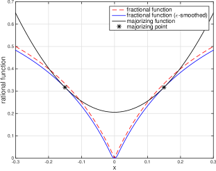
Fig. 1: Majorization for smoothed sparsity-inducing function.

3.3 The Majorized Subproblem in MM

By combining $\overline{L}_{2}\left(\boldsymbol{\Pi},\boldsymbol{\theta}^{\left(k\right)}\right)$ and $\overline{R}\left(\boldsymbol{\Pi},\boldsymbol{\theta}^{\left(k\right)}\right)$, we can get the majorizing function for $\overline{F}\left(\boldsymbol{\theta}\right)$ which is given as follows:

$$\begin{array}[]{l}\overline{F}_{1}\left(\boldsymbol{\Pi},\boldsymbol{\theta}^{\left(k\right)}\right)\simeq\overline{L}_{2}\left(\boldsymbol{\Pi},\boldsymbol{\theta}^{\left(k\right)}\right)+\xi\overline{R}\left(\boldsymbol{\Pi},\boldsymbol{\theta}^{\left(k\right)}\right)\\ \simeq\frac{1}{2}\mathrm{vec}\left(\boldsymbol{\Pi}\right)^{T}\mathbf{G}^{\left(k\right)}\mathrm{vec}\left(\boldsymbol{\Pi}\right)-\mathrm{vec}\left(\mathbf{H}^{\left(k\right)}\right)^{T}\mathrm{vec}\left(\boldsymbol{\Pi}\right),\end{array}$$

where $\mathbf{G}^{\left(k\right)}=\bar{\mathbf{Y}}_{-1}\bar{\mathbf{M}}\bar{\mathbf{Y}}_{-1}^{T}\otimes\boldsymbol{\Sigma}^{-\left(k\right)}+\xi\mathrm{diag}\left(\mathbf{q}^{\left(k\right)}\right)\otimes\mathbf{I}_{K}$, and $\mathbf{H}^{\left(k\right)}=\boldsymbol{\Sigma}^{-\left(k\right)}\Delta\bar{\mathbf{Y}}\bar{\mathbf{M}}\bar{\mathbf{Y}}_{-1}^{T}$. Although $\overline{F}_{1}\left(\boldsymbol{\Pi},\boldsymbol{\theta}^{\left(k\right)}\right)$ is a quadratic function in $\boldsymbol{\Pi}$, together with the nonconvex rank constraint on $\boldsymbol{\Pi}$ in (5), the problem is still hard to solve.

Lemma 4.

Let $\mathbf{A},\mathbf{B}\in\mathbb{S}^{K}$ and $\mathbf{B}\succeq\mathbf{A}$, then at any point $\mathbf{x}^{\left(k\right)}\in\mathbb{R}^{K}$, $\mathbf{x}^{T}\mathbf{A}\mathbf{x}\leq\mathbf{x}^{T}\mathbf{B}\mathbf{x}+2\mathbf{x}^{\left(k\right)T}\left(\mathbf{A}-\mathbf{B}\right)\mathbf{x}+\mathbf{x}^{\left(k\right)T}\left(\mathbf{B}-\mathbf{A}\right)\mathbf{x}^{\left(k\right)}$ with the equality attained at $\mathbf{x}=\mathbf{x}^{\left(k\right)}$.

Based on Lemma 4 and noticing $\psi_{\mathbf{G}}^{\left(k\right)}\mathbf{I}_{K^{2}}\succeq\mathbf{G}^{\left(k\right)}$ for any $\psi_{\mathbf{G}}^{\left(k\right)}$ satisfying $\psi_{\mathbf{G}}^{\left(k\right)}\geq\lambda_{\max}\left(\mathbf{G}^{\left(k\right)}\right)$, $\overline{F}_{1}\left(\boldsymbol{\Pi},\boldsymbol{\theta}^{\left(k\right)}\right)$ can be further majorized by the following function:

$$\begin{array}[]{l}\overline{F}_{2}\left(\boldsymbol{\Pi},\boldsymbol{\theta}^{\left(k\right)}\right)\simeq\frac{1}{2}\psi_{\mathbf{G}}^{\left(k\right)}\left\|\boldsymbol{\Pi}-\mathbf{P}^{\left(k\right)}\right\|_{F}^{2},\end{array}$$

where $\mathbf{P}^{\left(k\right)}=\boldsymbol{\Pi}^{\left(k\right)}-\psi_{\mathbf{G}}^{-\left(k\right)}\boldsymbol{\Sigma}^{-\left(k\right)}\boldsymbol{\Pi}^{\left(k\right)}\bar{\mathbf{Y}}_{-1}\bar{\mathbf{M}}\bar{\mathbf{Y}}_{-1}^{T}-\xi\psi_{\mathbf{G}}^{-\left(k\right)}\boldsymbol{\Pi}^{\left(k\right)}\mathrm{diag}\left(\mathbf{q}^{\left(k\right)}\right)+\psi_{\mathbf{G}}^{-\left(k\right)}\mathbf{H}^{\left(k\right)}$.

Finally, the majorized subproblem for problem (5) is

$$\begin{array}[]{c}\underset{\boldsymbol{\Pi}}{\mathsf{minimize}}\>\left\|\boldsymbol{\Pi}-\mathbf{P}^{\left(k\right)}\right\|_{F}^{2}\;\mathsf{subject\,to}\>\mathrm{rank}\left(\boldsymbol{\Pi}\right)\leq r.\end{array}$$ (6)

This problem has a closed form solution. Let the singular value decomposition for $\mathbf{P}$ be $\mathbf{P}=\mathbf{U}\mathbf{S}\mathbf{V}^{T}$, the optimal $\boldsymbol{\Pi}$ is $\boldsymbol{\Pi}^{\star}=\mathbf{U}\mathbf{S}_{r}\mathbf{V}^{T}$, where $\mathbf{S}_{r}$ is obtained by thresholding the smallest $\left(P-r\right)$ diagonal elements in $\mathbf{S}$ to be zeros. Accordingly, parameters $\boldsymbol{\alpha}$ and $\boldsymbol{\beta}$ can be factorized by $\boldsymbol{\Pi}^{\star}=\boldsymbol{\alpha}^{\star}\boldsymbol{\beta}^{\star T}$.

3.4 The MM-RSVECM Algorithm

Based on the MM method, to solve the original problem (5), we just need to iteratively solve a low-rank approximation problem (6) with a closed form solution at each iteration. The overall algorithm is summarized in Algorithm 1.

Input: $\left\{\mathbf{y}_{i}\right\}_{i=1}^{N}$ and needed pre-sampled values.

Initialization: $\boldsymbol{\Pi}^{\left(0\right)}\left(\boldsymbol{\alpha}^{\left(0\right)},\boldsymbol{\beta}^{\left(0\right)}\right)$, $\boldsymbol{\Gamma}^{\left(0\right)}$, $\boldsymbol{\Sigma}^{\left(0\right)}$ and $k=1$.

Repeat

1. Compute $\mathbf{w}^{\left(k\right)}$, $\mathbf{q}^{\left(k\right)}$, $\mathbf{G}^{\left(k\right)}$, $\mathbf{H}^{\left(k\right)}$, $\psi_{\mathbf{G}}^{\left(k\right)}$ and $\mathbf{P}^{\left(k\right)}$;

2. Update $\boldsymbol{\Pi}^{\left(k\right)}$ by solving (6) and $\boldsymbol{\Gamma}^{\left(k\right)}$, $\boldsymbol{\Sigma}^{\left(k\right)}$;

3. $k=k+1$;

Until $\boldsymbol{\Pi}^{\left(k\right)}$, $\boldsymbol{\Gamma}^{\left(k\right)}$ and $\boldsymbol{\Sigma}^{\left(k\right)}$ satisfy a termination criterion.

Output: $\hat{\boldsymbol{\Pi}}\left(\hat{\boldsymbol{\alpha}},\hat{\boldsymbol{\beta}}\right)$, $\hat{\boldsymbol{\Gamma}}$ and $\hat{\boldsymbol{\Sigma}}$.

Algorithm 1 MM-RSVECM - Robust MLE of Sparse VECM

4 Numerical Simulations

Numerical simulations are considered in this section. A VECM $\left(K=5,\>r=3,\>N=1000\right)$ with underlying group sparse structure for $\boldsymbol{\Pi}$ is specified firstly. Then a time series sample path is generated with innovations distributed to Student $t$-distribution with degree of freedom $p=3$. We first compare our algorithm (MM-RSVECM) with the gradient descent algorithm (GD-RSVECM) for the proposed nonconvex problem formulation in (5). The convergence result of the objective function value is shown in Fig. 2.

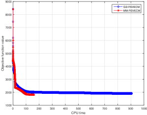
Fig. 2: Convergence comparison for objective function value.

Based on the MM method, MM-RSVECM obtains a faster convergence than GD-RSVECM. This may be because the algorithm based on the MM method better exploits the structure of the original problem.

Then the proposed problem formulation based on Cauchy log-likelihood loss function is further validated by comparing the parameter estimation accuracy under student $t$-distributions with different degree of freedom $p$. The estimation accuracy is measure by the normalized mean squared error (NMSE):

$$\text{NMSE}\left(\boldsymbol{\Pi}\right)=\frac{\mathbb{E}\left[\left\|\hat{\boldsymbol{\Pi}}-\boldsymbol{\Pi}_{\mathrm{true}}\right\|_{F}^{2}\right]}{\left\|\boldsymbol{\Pi}_{\mathrm{true}}\right\|_{F}^{2}}.$$

In Fig. 3, we show the simulation results for $\text{NMSE}\left(\boldsymbol{\Pi}\right)$ by using three estimation methods, which are based on Gaussian innovation assumption, true Student $t$-distribution, and the proposed Cauchy innovation assumption.

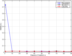
Fig. 3: $\text{NMSE}\left(\boldsymbol{\Pi}\right)$ vs degree of freedom $p$ for $t$-distributions.

From Fig. 3, we can see the parameter estimated from Cauchy assumption using the MM-VECM algorithm consistently has a lower parameter estimation error compared to the estimation results from Gaussian assumption and even using the true Student $t$-distribution. Based on this, the proposed problem formulation is validated.

5 Conclusions

This paper has considered the robust and sparse VECM estimation problem. The problem has been formulated by considering a robust Cauchy log-likelihood loss function and a nonconvex group sparsity regularizer. An efficient algorithm based on the MM method has been proposed with the efficiency of the algorithm and the estimation accuracy validated through numerical simulations.

References

- [1] H. Lütkepohl, New introduction to multiple time series analysis. Springer, 2007.
- [2] C. W. Granger, “Cointegrated variables and error correction models,” unpublished USCD Discussion Paper 83-13a, Tech. Rep., 1983.
- [3] R. F. Engle and C. W. Granger, “Co-integration and error correction: representation, estimation, and testing,” Econometrica: Journal of the Econometric Society, pp. 251–276, 1987.
- [4] S. Johansen, “Statistical analysis of cointegration vectors,” Journal of Economic Dynamics and Control, vol. 12, no. 2, pp. 231–254, 1988.
- [5] ——, “Estimation and hypothesis testing of cointegration vectors in gaussian vector autoregressive models,” Econometrica: Journal of the Econometric Society, pp. 1551–1580, 1991.
- [6] ——, “Identifying restrictions of linear equations with applications to simultaneous equations and cointegration,” Journal of Econometrics, vol. 69, no. 1, pp. 111–132, 1995.
- [7] A. Pole, Statistical arbitrage: algorithmic trading insights and techniques. John Wiley & Sons, 2011, vol. 411.
- [8] S. T. Rachev, C. Menn, and F. J. Fabozzi, Fat-tailed and skewed asset return distributions: implications for risk management, portfolio selection, and option pricing. John Wiley & Sons, 2005, vol. 139.
- [9] P. H. Franses and N. Haldrup, “The effects of additive outliers on tests for unit roots and cointegration,” Journal of Business & Economic Statistics, vol. 12, no. 4, pp. 471–478, 1994.
- [10] P. H. Franses, T. Kloek, and A. Lucas, “Outlier robust analysis of long-run marketing effects for weekly scanning data,” Journal of Econometrics, vol. 89, no. 1, pp. 293–315, 1998.
- [11] H. B. Nielsen, “Cointegration analysis in the presence of outliers,” The Econometrics Journal, vol. 7, no. 1, pp. 249–271, 2004.
- [12] A. Lucas, “Unit root tests based on m estimators,” Econometric Theory, vol. 11, no. 02, pp. 331–346, 1995.
- [13] ——, “An outlier robust unit root test with an application to the extended nelson-plosser data,” Journal of Econometrics, vol. 66, no. 1, pp. 153–173, 1995.
- [14] P. H. Franses and A. Lucas, “Outlier detection in cointegration analysis,” Journal of Business & Economic Statistics, vol. 16, no. 4, pp. 459–468, 1998.
- [15] A. Lucas, “Cointegration testing using pseudolikelihood ratio tests,” Econometric Theory, pp. 149–169, 1997.
- [16] F. Bach, R. Jenatton, J. Mairal, G. Obozinski et al., “Optimization with sparsity-inducing penalties,” Foundations and Trends® in Machine Learning, vol. 4, no. 1, pp. 1–106, 2012.
- [17] R. Tibshirani, “Regression shrinkage and selection via the lasso,” Journal of the Royal Statistical Society. Series B (Methodological), pp. 267–288, 1996.
- [18] I. Wilms and C. Croux, “Forecasting using sparse cointegration,” International Journal of Forecasting, vol. 32, no. 4, pp. 1256–1267, 2016.
- [19] L. Chen and J. Z. Huang, “Sparse reduced-rank regression for simultaneous dimension reduction and variable selection,” Journal of the American Statistical Association, vol. 107, no. 500, pp. 1533–1545, 2012.
- [20] ——, “Sparse reduced-rank regression with covariance estimation,” Statistics and Computing, vol. 26, no. 1-2, pp. 461–470, 2016.
- [21] D. Geman and G. Reynolds, “Constrained restoration and the recovery of discontinuities,” IEEE Transactions on Pattern Analysis and Machine Intelligence, vol. 14, no. 3, pp. 367–383, 1992.
- [22] B. Bosco, L. Parisio, M. Pelagatti, and F. Baldi, “Long-run relations in European electricity prices,” Journal of Applied Econometrics, vol. 25, no. 5, pp. 805–832, 2010.
- [23] M. A. Figueiredo, J. M. Bioucas-Dias, and R. D. Nowak, “Majorization-minimization algorithms for wavelet-based image restoration,” IEEE Transactions on Image Processing, vol. 16, no. 12, pp. 2980–2991, 2007.
- [24] D. R. Hunter and K. Lange, “A tutorial on MM algorithms,” The American Statistician, vol. 58, no. 1, pp. 30–37, 2004.
- [25] M. Razaviyayn, M. Hong, and Z.-Q. Luo, “A unified convergence analysis of block successive minimization methods for nonsmooth optimization,” SIAM Journal on Optimization, vol. 23, no. 2, pp. 1126–1153, 2013.
- [26] Y. Sun, P. Babu, and D. P. Palomar, “Majorization-minimization algorithms in signal processing, communications, and machine learning,” IEEE Transactions on Signal Processing, vol. 65, no. 3, pp. 794–816, 2016.