Study of Spin through Gluon Poles

Abstract

Based on the use of contour gauge and collinear factorization, we propose a new set of single spin asymmetry which can be measured in polarized Drell-Yan process by SPD@NICA. We stress that all of discussed single spin asymmetries exist owing to the gluon poles manifesting in the twist-3 or twist-2$\otimes$twist-3 parton distributions related to the transverse-polarized Drell-Yan process.

1 Introduction

The studies of hadron structure are based on the investigations of both semi-inclusive and exclusive processes which can be described by transverse momentum dependent (TMDs) and generalized parton distributions (GPDs). The duality and matching between different factorization regimes are one of importances for the coherent QCD description of hadron structure. We discuss the manifestation of such effects in the pion-nucleon Drell-Yan process at large $x_{F}$ provided pions are described by wave functions and distribution amplitudes rather than parton distributions.

We calculate the gauge invariant Drell-Yan-like hadron tensors. In connection with new COMPASS results, we predict the new single spin asymmetry which probes gluon poles together with chiral-odd and time-odd functions. The relevant pion production as a particular case of Drell-Yan-like process has been discussed. For the meson-induced Drell-Yan process, we model an analog of the twist three distribution function, which is a collinear function in inclusive channel, by means of two non-collinear distribution amplitudes which are associated with exclusive channel. This modelling demonstrates the fundamental duality between different factorization regimes.

2 Drell-Yan-like processes: new result for pion-nucleon Drell-Yan process

We study the process which has the following schematic representation, see Fig.1

$$A^{(\uparrow\downarrow)}(p_{1})+B(p_{2})\to\gamma^{*}(q)+X(P_{X})\to\ell(l_{1})+\bar{\ell}(l_{2})+X(P_{X}),$$ (1)

where $A$ denotes the (transverse)polarized nucleon, $B$ stands for an arbitrary hadron and $l_{1}+l_{2}=q$ has a large mass squared ($q^{2}=Q^{2}$). The single transverse spin asymmetry (SSA) under our consideration is given by

$${\cal A}=\frac{d\sigma^{(\uparrow)}-d\sigma^{(\downarrow)}}{d\sigma^{(\uparrow)}+d\sigma^{(\downarrow)}},\quad\frac{d\sigma^{(\uparrow\downarrow)}}{d^{4}qd\Omega}=\frac{\alpha^{2}_{em}}{2jq^{4}}{\cal L}_{\mu\nu}\,H_{\mu\nu}\,,$$ (2)

where ${\cal L}_{\mu\nu}$ is a lepton tensor, and $H_{\mu\nu}$ - the QED gauge invariant hadron tensor which corresponds to the difference between direct and mirror channels in the regime of $x_{F}\to 1$.

         

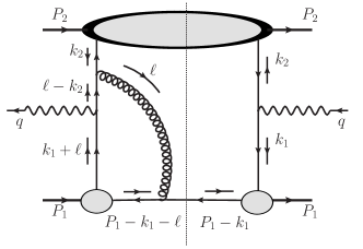
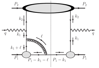
Figure 1: The Feynman diagrams which contribute to the polarized Drell-Yan hadron tensor: the left panel corresponds to the standard diagram while the right panel – to the nonstandard diagram. Note that the standard and nonstandard diagrams differ by the hard parts [1].

In Fig.1, the upper blob with the light-cone minus dominant direction is given by the following hadron matrix element:

$$\langle P_{2},S_{\perp}|\big{[}\bar{\psi}\,\sigma^{-\perp}\,\psi\big{]}^{\text{tw-2}}|S_{\perp},P_{2}\rangle\stackrel{{\scriptstyle{\cal F}}}{{\sim}}\varepsilon^{-\perp S^{\perp}P_{2}}\,\bar{h}_{1}(y)$$ (3)

and the lower blob with the light-cone plus dominant direction corresponds to

$$\langle P_{1},S|\big{[}\bar{\psi}\,\gamma^{+}\,A^{\alpha}_{\perp}\,\psi\big{]}^{\text{tw-3}}|S,P_{1}\rangle\Big{|}_{\text{DY}}\Longrightarrow$$ (4)

$${\cal D}^{\alpha\beta}\,\langle 0|\big{[}\bar{\psi}\gamma^{+}(\gamma_{5})\psi\big{]}^{\text{tw-2}}|S,P_{1}\rangle\,\gamma_{\beta}\,\langle P_{1},S|\big{[}\bar{\psi}\sigma^{-+}(\gamma_{5})\psi\big{]}^{\text{tw-3}}|0\rangle\Big{|}_{\pi N\text{-DY}}$$

which finally leads to (see, [2, 3, 4, 5, 6] for details)

$$\widetilde{B}(x_{1},x_{2})=\frac{1}{2}\frac{\Phi_{(1)}^{\text{tw-3}}(x_{1})\stackrel{{\scriptstyle\hskip 5.69046pt\vec{\bf k}_{1}^{\,\perp}}}{{\circledast}}\Phi_{(2)}^{\text{tw-2}}(x_{2})}{x_{2}-x_{1}-i\epsilon}\,.$$ (5)

where $-i\epsilon$ stems from the contour gauge: $[z^{-},-\infty^{-}]_{A^{+}}=1$.

For the chiral-odd contributions, within our framework, we predict a new SSA which reads

$${\cal A}_{T}=\frac{S_{\perp}}{Q}\,\frac{D_{[\sin 2\theta]}\,\sin\phi_{S}B^{\sin\phi_{S}}_{UT}}{\bar{f}_{1}(y_{B})\,H_{1}(x_{B})},\,D_{[\sin 2\theta]}=\frac{\sin 2\theta}{1+\cos^{2}\theta}$$ (6)

where

$$B^{\sin\phi_{S}}_{UT}=2\bar{h}_{1}(y_{B})\,\Phi_{(1)}^{\text{tw-3}}(x_{B})\stackrel{{\scriptstyle\hskip 5.69046pt\vec{\bf k}_{1}^{\,\perp}}}{{\circledast}}\Phi_{(2)}^{\text{tw-2}}(x_{B})$$ (7)

and $\bar{f}_{1}(y_{B}),\,H_{1}(x_{B})$ emanate from the unpolarized cross-section and they parameterize the following matrix elements. The result is presented in terms of [7]. We want to emphasize that the predicted SSA (6) exists due to the complexity of $\widetilde{B}(x_{1},x_{2})$-function (5), i.e. $\Im\text{m}\widetilde{B}(x_{1},x_{2})\neq 0$.

From comparison with recent COMPASS results on pion-nucleon Drell-Yan process, we can see that our ${\cal A}_{T}$ is completely new one. Indeed, the leading twist Sivers asymmetry $A^{\sin\phi_{S}}_{UT}$ which formally stands at the similar tensor combination $\varepsilon^{l^{\perp}_{1}S^{\perp}P_{1}P_{2}}$, appears only together with the depolarization factor $D_{[1+\cos^{2}\theta]}$. In its turn, the higher twist asymmetries $A^{\sin(\phi_{S}\pm\phi)}_{UT}$ at $D_{[\sin 2\theta]}$ correspond to the different tensor structures, $\varepsilon^{qS^{\perp}P_{1}^{\perp}P_{2}}\sim\sin(\phi_{S}\pm\phi)$.

3 Factorization theorem, in a nutshell

Since the main our tool is the factorization procedure, let us outline the principal items of factorization we adhere. With a help of factorization, a given amplitude of hadron tensor of any hard processes can be estimated, not calculated, by the well-defined procedure within the corresponding asymptotical regime. As a result of this estimation, we arrive at the well-known factorization theorem which states that the short (hard) and long (soft) distance dynamics can be separated out provided $Q^{2}$ is large, i.e.

$${\cal W}_{\mu\nu...}=\int d^{4}k_{1}d^{4}k_{2}...\,\text{tr}\big{[}\Phi_{1}(k_{1})E_{\mu\nu...}(k_{1},k_{2},...)\Phi_{2}(k_{2})...\big{]}\stackrel{{\scriptstyle Q^{2}\to\infty}}{{\Longrightarrow}}$$

$$\int dxdy...\,\text{tr}\big{[}\Phi_{1}(y)E_{\mu\nu}(x,y,...)\,\Phi_{2}(x)...\big{]}+{\cal O}(1/Q^{2})$$ (8)

where $E_{\mu\nu...}(k_{i})$ implies the products of propagators multiplying by the momentum conservation $\delta$-function, and

$$E_{\mu\nu}(x,y,...|{\bf k}^{T}_{i}=0),\quad\Phi(k)\stackrel{{\scriptstyle{\cal F}}}{{=}}\langle{\cal O}^{(\bar{\psi},\psi,A)}(z,0)\rangle\,,$$ (9)

$$\Phi(x_{i})=\int dk^{+}_{i}\,\delta(x_{i}-k^{+}_{i}\cdot n)\,\int dk^{-}_{i}\,d^{2}{\bf k}^{T}_{i}\,\Phi(k_{i})\,.$$ (10)

Besides, both the hard and soft parts should be independent of each other, UV- and IR-renormalizable and, finally, parton distributions must possess the universality property. We notice that the transverse momentum integral in (10) gives us the possibility for the study of TMDs. In the other words, the TMDs can contribute through the corresponding moments. However, if the nontrivial ${\bf k}^{T}_{i}$-dependence has been kept in $E_{\mu\nu}(x,y,...|{\bf k}^{T}_{i})$, the factorization theorem can be in question. It can be happened, for example, in case we want to restore the ${\bf k}^{T}$-dependent Wilson line in the correlators $\Phi(k_{i})$.

4 Contour gauge and complexity of $B(x_{1},x_{2})$-functions

We show that the contour gauges for gluon fields play the crucial role for our study. The contour gauge belongs to the class of non-local gauges that depends on the path connecting two points in the correlators. It turns out, in the cases which we consider, the prescriptions for the gluonic poles in the twist $3$ correlators, see (5), are dictated by the contour gauge $[x,\,\pm\infty]=1$. Indeed, one can easily check that the representation with $x_{1}-x_{2}+i\epsilon$ in the denominator belongs to the gauge $[x,\,-\infty]=1$, while the representation with $x_{1}-x_{2}-i\epsilon$ belongs to the gauge $[+\infty,\,x]=1$.

Thus, we find that the nonstandard new terms, which exist in the case of the complex twist-$3$ $B$-function with the corresponding prescriptions, do contribute to the hadron tensor exactly as the standard term known previously. This is another important result of our work.

In conclusion of this section, let us briefly discuss the main items of the contour gauge conception. To describe this class of gauges, we adhere the geometrical interpretation of gluons where the gluon field is a connection of the principal fiber bundle ${\cal P}(\mathbb{R}^{4},G,\pi)$. Here, $\mathbb{R}^{4}$ is the base where the principal fiber bundle is determined, $G$ denotes the group defined on the given fiber and $\pi$ is a transformation of the base $\mathbb{R}^{4}$ into the fiber bundle ${\cal P}$). The corresponding path-dependent Wilson factor (or line), representing each element $\textbf{g}(x)$ of the fiber, defines the gauge-transformed field:

$$A^{\textbf{g}}_{\mu}(x)=\textbf{g}^{-1}(x)A_{\mu}(x)\textbf{g}(x)+\frac{i}{g}\textbf{g}^{-1}(x)\partial_{\mu}\textbf{g}(x).$$ (11)

The set of these fields for all $\textbf{g}(x)$ forms the gauge orbit. In order to quantize a system of the gauge fields, one chooses the only element of each orbit. In contrast to the standard way, we first fix an arbitrary point $(x_{0},\textbf{g}(x_{0}))$ in the fiber. Then, we define two directions: one of them in the base, the other in the fiber. The direction in the base $\mathbb{R}^{4}$ is the tangent vector of a curve which goes through the given point $x_{0}$. At the same time, the direction in the fiber can be uniquely determined as the tangent subspace related to the parallel transition. Due to this procedure, we uniquely define the point in the fiber bundle.

Having solved the parallel transport equation defined on the fiber as

$$\frac{dx_{\alpha}(v)}{dv}\,{\cal D}_{\alpha}\textbf{g}(x(v))=0\,,$$ (12)

we find the solution in terms of the Wilson line:

$$\textbf{g}(x)=Pexp\Big{\{}ig\int\limits_{\mathbb{P}(x_{0},x)}d\omega\cdot A(\omega)\Big{\}}\textbf{g}(x_{0}),$$ (13)

where the points $x_{0}$ and $x$ are connected by the path $\mathbb{P}$. The starting point $x_{0}$ is usually fixed. Here, $\textbf{g}(x_{0})$ is chosen to be equal to unity. Note that the fixing of $\textbf{g}(x)$ ensures a unique choice of the element in the orbit. We now insert (13) into (11) and can see that the field $A^{\textbf{g}}_{\mu}(x)$ is completely determined by the form of the path which connects the starting and final points. Moreover, using (11) and (13), one obtains the property:

$$Pexp\Big{\{}ig\int\limits_{x_{0}}^{x}d\omega\cdot A^{\textbf{g}}(\omega)\Big{\}}=\textbf{g}^{-1}(x)Pexp\Big{\{}ig\int\limits_{x_{0}}^{x}d\omega\cdot A(\omega)\Big{\}}\textbf{g}(x_{0}).$$ (14)

Then, if we insert (13) into (11), we arrive at

$$A^{\textbf{g}}_{\mu}(x)=\int\limits_{\mathbb{P}(x_{0},x)}dz_{\alpha}\frac{\partial z_{\beta}}{\partial x_{\mu}}\,\textbf{g}^{-1}(z)\,G_{\alpha\beta}(z|A)\,\textbf{g}(z)=\int\limits_{\mathbb{P}(x_{0},x)}dz_{\alpha}\frac{\partial z_{\beta}}{\partial x_{\mu}}\,G_{\alpha\beta}(z|A^{\textbf{g}}),$$ (15)

where

$$G_{\alpha\beta}(z|A^{\textbf{g}})\equiv G_{\alpha\beta}^{\textbf{g}}(z)=\textbf{g}^{-1}(z)\,G_{\alpha\beta}(z|A)\,\textbf{g}(z)$$ (16)

The contour gauge condition demands that $\textbf{g}(x)$ is equal to unity for all $x$ belonging to the base, i.e.

$$[x,\,x_{0}]\stackrel{{\scriptstyle def}}{{=}}Pexp\Big{\{}ig\int\limits_{x_{0}}^{x}d\omega\cdot A(\omega)\Big{\}}=1,\,\,\,\forall x\in\mathbb{R}^{4}.$$ (17)

Therefore, within the contour gauge, the field $A^{\textbf{g}}_{\mu}$ (see, (15)) becomes

$$A^{c.g.}_{\mu}(x)=\int\limits_{\mathbb{P}(x_{0},x)}dz_{\alpha}\frac{\partial z_{\beta}}{\partial x_{\mu}}\,G_{\alpha\beta}(z|A^{c.g.}),$$ (18)

i.e. the gluon field $A^{\textbf{g}}_{\mu}$ is a linear functional of the tensor $G_{\mu\nu}$.

5 Conclusions

To conclude we derive the gauge invariant meson-induced DY hadron tensor with the essential spin transversity and primordial transverse momenta. Our calculation includes both the standard-like, which is well-known, and nonstandard-like diagram, which is first found in [4], contributions. The latter contribution plays a crucial role for the gauge invariance.

We study the case of pion distribution amplitudes which has been projected onto the chiral-odd combination. The latter singles out the chiral-odd parton distribution inside nucleons. The chiral-odd tensor combinations are very relevant for the future experiments implemented by COMPASS [7]. We predict a new single transverse spin asymmetry which can be measured experimentally, for example, by SPD@NICA. The latter asymmetry can eventually be treated as a signal for the transverse “primordial” momentum dependence which probes both gluon poles and time-odd functions.

We thank A.V. Efremov, L. Motyka and A. P. Nagaytsev for useful discussions. The work by I.V.A. was partially supported by the Bogoliubov-Infeld Program and Heisenberg-Landau Program HL-2017. L.Sz. is partly supported by grant No $2015/17/\text{B}/\text{ST}2/01838$ from the National Science Center in Poland.

References

References

• [1] I. V. Anikin and O. V. Teryaev 2009 Phys. Part. Nucl. Lett. 6 3
• [2] I. V. Anikin, L. Szymanowski, O. V. Teryaev and N. Volchanskiy 2017 Phys. Rev. D 95 111501
• [3] I. V. Anikin, I. O. Cherednikov and O. V. Teryaev 2017 Phys. Rev. D 95 034032
• [4] I. V. Anikin and O. V. Teryaev 2010 Phys. Lett. B 690 519
• [5] I. V. Anikin and O. V. Teryaev 2015 Eur. Phys. J. C 75 184
• [6] I. V. Anikin and O. V. Teryaev 2015 Phys. Lett. B 751 495
• [7] M. Aghasyan et al. [COMPASS Collaboration] 2017 arXiv:1704.00488 [hep-ex].