Quenched dynamics of entangled states in correlated quantum dots

Abstract

Time evolution of initially prepared entangled state in the system of coupled quantum dots has been analyzed by means of two different theoretical approaches: equations of motion for the all orders localized electron correlation functions, considering interference effects, and kinetic equations for the pseudo-particle occupation numbers with constraint on the possible physical states. Results obtained by means of different approaches were carefully analyzed and compared with each other. Revealed direct link between concurrence (degree of entanglement) and quantum dots pair correlation functions allowed us to follow the changes of entanglement during time evolution of the coupled quantum dots system. It was demonstrated that the degree of entanglement can be controllably tuned during the time evolution of quantum dots system.

I Introduction

One of the most interesting problems in the present-day nanophysics is the controllable formation of entangled electronic states for use in quantum information processing and cryptography. Coupled quantum dots (QDs) systems recently seem to be promising candidates for quantum information applications as single and two-electronic states can be well initialized, processed and readout in such ultra-small structures Loss ; Imamoglu ; Yao ; Blaauboer ; Robledo ; Nowack ; Schulman ; Maslova .

Properties of entangled states are usually analyzed in the stationary case. However, time evolution of spin and charge configurations, initially prepared in coupled QDs, is also of great interest as non-stationary characteristics could reveal new information about the physical properties of nanoscale systems in addition to the stationary ones Bar-Joseph ; Gurvitz_1 ; Arseyev_1 ; Mantsevich ; Arseyev_2 ; Stafford_1 ; Hazelzet ; Cota . Kinetics of initially prepared charge and spin states in quantum dots systems is strongly governed by the high order localized electrons correlation functions due to the presence of Coulomb interaction Arseyev_3 and is also influenced by the interference effects between electrons traveling through different paths Wiel ; Okazaki ; Amasha .

One of the challenges in the area of non-stationary electron transport through coupled QDs is to prepare interacting few-level systems with different initial states Bayer ; Creatore ; Tsukanov ; Yokoshi - from simple product states to complex entanglements. Various ideas for entangling of spatially separated electrons were proposed, such as, by splitting Cooper pairs Burkard or by spin manipulation in QDs Sanchez ,Ciccarello . In double correlated QDs entangled state can appear as an eigenstate with particular number of electrons Blaauboer ,Burkard_1 or by sending an electrical current through the nano-scale structure Busser . There are a lot of possible applications of entangled states in nano-electronics Dowling , including quantum information processing Nielsen . Most of the proposed schemes for quantum computation deal with the spin control due to the localized spins long decoherence times Hanson . As it was recently shown, entangled states in correlated QDs could reveal long relaxation times due to the particular symmetry of investigated system. Moreover, entangled states in correlated quantum dots can be well controlled by applied bias voltage changing Murgida ,Kataoka or by external laser pulses Putaja ,Saelen .

Recently the potential of quantum information processing and quantum computation results in numerous proposals of specific material systems for creation and manipulation of entanglement in solid state. System based on the coupled quantum dots with Coulomb correlations has several appealing features: 1) single spin is a natural qubit, 2) presence of strong Coulomb interaction within the system creates entanglement even in the most easily experimentally obtained ground state, 3) entangled quantum states in the coupled QDs can be experimentally realized without such restrictions as for two-impurity Kondo model. Moreover, the degree of entanglement can change during the relaxation of initially prepared charge state in double QD coupled to reservoir Maslova .

In the present paper we analyze time evolution of initially prepared entangled state in the correlated double QD due to the interaction with an electronic reservoir. Two different approaches were considered: the first one is based on the equations of motion for all orders localized electron correlation functions and the second one deals with the kinetic equations for pseudo-particle occupation numbers, considering constraint on the possible physical states. Results, obtained by means of these approaches were carefully analyzed and compared with each other. It was demonstrated that both approaches allow one to follow the changes of the system entanglement during time evolution due to the direct link between concurrence and quantum dots pair correlation functions. For different initial mixed states entanglement could reveal non-monotonic behavior and even increase considerably during the relaxation processes in coupled quantum dots in the particular time interval. So, one can tune the degree of entanglement during the time evolution of correlated QDs. Proposed system is a good candidate for quantum information protocol (QIP) realization with the help of scanning tunneling microscopy/spectroscopy technique.

II Theoretical model

We consider a system of two coupled correlated QDs connected to an electronic reservoir. The Hamiltonian $\hat{H_{D}}$, describing interacting quantum dots reads

$$\hat{H}_{D} = \sum_{l=1,2,\sigma}\varepsilon_{l}c^{+}_{l\sigma}c_{l\sigma}+\sum_{l=1,2}U_{l}n_{ll}^{\sigma}n_{ll}^{-\sigma}+$$ (1)

$$+ \sum_{\sigma}T(c_{1\sigma}^{+}c_{2\sigma}+c_{1\sigma}c_{2\sigma}^{+}),$$

where $\varepsilon_{l}$ ($l=1,2$) are the spin-degenerate single-electron energy levels and $U_{l}$ is the on-site Coulomb repulsion for the quantum dots double occupation. Creation/annihilation of an electron with spin $\sigma=\pm 1$ within the dot is denoted by operators $c^{+}_{l\sigma}/c_{l\sigma}$ and $n_{ll}^{\sigma}$ is the corresponding occupation number operator. Coupling between the dots is described by tunneling transfer amplitude $T$ which is considered to be independent on momentum and spin.

Reservoir is modeled by the Hamiltonian:

$$\hat{H}_{res}=\sum_{k\sigma}\varepsilon_{k}c^{+}_{k\sigma}c_{k\sigma},$$ (2)

where operator $c^{+}_{k\sigma}/c_{k\sigma}$ creates/annihilates an electron with spin $\sigma$ and momentum $k$ in the lead. Coupling between both dots and reservoir is described by the Hamiltonian:

$$\hat{H}_{tun}=\sum_{k\sigma}t(c_{k\sigma}^{+}c_{l\sigma}+c_{l\sigma}^{+}c_{k\sigma}).$$ (3)

Tunneling amplitude $t$ is independent on momentum and spin. When coupling between QDs exceeds the value of interaction with the reservoir, one can use the basis of exact eigenfunctions and eigenvalues of coupled QDs without interaction with the leads. In this case all energies of single- and multi-electron states are well known.

Two single electron states are present in the system and can be described by the wave function

$$\Psi_{i}^{\sigma}=\mu_{i}\cdot|0\uparrow\rangle|00\rangle+\nu_{i}\cdot|00\rangle|0\uparrow\rangle,$$ (4)

where basis functions $|0\uparrow\rangle|00\rangle$ and $|00\rangle|0\uparrow\rangle$ describe the existence of single electron with a given spin in each quantum dot. Single electron energies

$$\varepsilon_{a(s)}=\frac{\varepsilon_{1}+\varepsilon_{2}}{2}\pm\sqrt{\frac{(\varepsilon_{1}-\varepsilon_{2})^{2}}{4}+T^{2}}$$ (5)

and coefficients $\mu_{i}$ and $\nu_{i}$ are determined by the eigenstates of matrix:

$$\begin{pmatrix}\varepsilon_{1}&&-T\\ -T&&\varepsilon_{2}\end{pmatrix}.$$ (6)

Six two electron states exist in the system: two states with the same electrons spin in each dot are given by the wave functions $T^{+}=|\uparrow 0\rangle|\uparrow 0\rangle$ and $T^{-}=|\downarrow 0\rangle|\downarrow 0\rangle$. Such states can be formed only by electrons localized in the different dots. Four states with the opposite spins can be described by the wave function

$$\Psi_{j}^{\sigma-\sigma} = \alpha_{j}\cdot|\uparrow\downarrow\rangle|00\rangle+\beta_{j}\cdot|\downarrow 0\rangle|0\uparrow\rangle+$$

$$+ \gamma_{j}\cdot|0\uparrow\rangle|\downarrow 0\rangle+\delta_{j}\cdot|00\rangle|\uparrow\downarrow\rangle,$$

where basis wave functions $|\uparrow\downarrow\rangle|00\rangle$; $|00\rangle|\uparrow\downarrow\rangle$ correspond to electrons localized in the same quantum dot - the first one or the second one and functions $|\downarrow 0\rangle|0\uparrow\rangle$; $|0\uparrow\rangle|\downarrow 0\rangle$ describe the situation when electrons are localized in different dots. Two electron states energies and coefficients $\alpha_{j}$, $\beta_{j}$, $\gamma_{j}$, $\delta_{j}$ are determined by the eigenvalues and eigenvectors of matrix:

$$\begin{pmatrix}2\varepsilon_{1}+U_{1}&&-T&&-T&&0\\ -T&&\varepsilon_{1}+\varepsilon_{2}&&0&&-T\\ -T&&0&&\varepsilon_{1}+\varepsilon_{2}&&0\\ 0&&-T&&-T&&2\varepsilon_{2}+U_{2}\end{pmatrix}.$$ (8)

These are low energy singlet $S^{0}$ and triplet $T^{0}$ states and excited singlet ($S^{0*}$) and triplet states ($T^{0*}$). Low energy triplet state $T^{0}$ with energy $\varepsilon_{1}+\varepsilon_{2}$ exists for any values of QDs energy levels $\varepsilon_{l}$ and Coulomb interaction $U_{l}$. Corresponding coefficients in Eq.(II) are $\alpha=\delta=0$ and $\beta=-\gamma=\frac{1}{\sqrt{2}}$.

Two three electron states with the wave function

$$\Psi_{m}^{\sigma\sigma-\sigma} = p_{m}|\uparrow\downarrow\rangle|\uparrow 0\rangle+q_{m}|\uparrow 0\rangle|\uparrow\downarrow\rangle$$

$$m = \pm 1$$ (9)

are present in the system. In this case basis functions $|\uparrow\downarrow\rangle|\uparrow 0\rangle$ and $|\uparrow 0\rangle|\uparrow\downarrow\rangle$ describe the situation, when one of the dots is fully occupied by two electrons with opposite spins and only single electron with a given spin is present in another dot. Coefficients $p_{m}$, $q_{m}$ and energies are determined by the eigenvectors and eigenvalues of matrix:

$$\begin{pmatrix}2\varepsilon_{1}+\varepsilon_{2}+U_{1}&&-T\\ -T&&2\varepsilon_{2}+\varepsilon_{1}+U_{2}\end{pmatrix}.$$ (10)

Finally, single four-electron state exists in the system with the wave function

$$\Psi_{n}=|\uparrow\downarrow\rangle|\uparrow\downarrow\rangle.$$ (11)

In this case both quantum dots are fully occupied.

II.1 Equations of motion for localized electron correlation functions

Coupling to reservoir leads to the changing of the dots occupation due to the tunneling processes. We now derive kinetic equations for bilinear combinations of the Heisenberg operators $c_{l\sigma}^{+}/c_{l\sigma}$, which allow to analyze the dynamics of localized electron occupation numbers and high order correlation functions due to the coupling to reservoir:

$$c_{1\sigma}^{+}c_{1\sigma}=\hat{n}_{11}^{\sigma}(t);\quad c_{2\sigma}^{+}c_{2\sigma}=\hat{n}_{22}^{\sigma}(t);$$

$$c_{1\sigma}^{+}c_{2\sigma}=\hat{n}_{12}^{\sigma}(t);\quad c_{2\sigma}^{+}c_{1\sigma}=\hat{n}_{21}^{\sigma}(t).$$ (12)

We consider time evolution of initially prepared state in the case of ”empty” reservoir in a wide band limit approximation and for deep energy levels ($\frac{|\varepsilon_{i}-\varepsilon_{F}|}{\Gamma}>>1$, where $\Gamma=\pi\nu_{0}t^{2}$, $\nu_{0}$ - is unperturbated density of states in the reservoir) when applied bias is equal to zero.

By means of Heisenberg equations of motion one can get closed system of equations for localized electrons occupation numbers exactly taking into account correlations of all orders Mantsevich ,Arseyev_2 (for weak tunneling coupling between QDs and reservoir). Kinetic equations describe time evolution of the electron occupation numbers in the proposed system:

$$\frac{\partial}{\partial t}\hat{n}_{11}^{\sigma} = -\Gamma(\hat{n}_{21}^{\sigma}+\hat{n}_{12}^{\sigma})+iT(\hat{n}_{21}^{\sigma}-\hat{n}_{12}^{\sigma})-2\Gamma\hat{n}_{11}^{\sigma},$$

$$\frac{\partial}{\partial t}\hat{n}_{22}^{\sigma} = -\Gamma(\hat{n}_{21}^{\sigma}+\hat{n}_{12}^{\sigma})-iT(\hat{n}_{21}^{\sigma}-\hat{n}_{12}^{\sigma})-2\Gamma\hat{n}_{22}^{\sigma},$$

$$\frac{\partial}{\partial t}\hat{n}_{21}^{\sigma} = -\Gamma(\hat{n}_{11}^{\sigma}+\hat{n}_{22}^{\sigma})+iT(\hat{n}_{11}^{\sigma}-\hat{n}_{22}^{\sigma})-i(\xi-2i\Gamma)\hat{n}_{21}^{\sigma}-$$

$$- iU_{11}n_{21}^{\sigma}n_{11}^{-\sigma}+iU_{22}n_{21}^{\sigma}n_{22}^{-\sigma},$$

$$\frac{\partial}{\partial t}\hat{n}_{12}^{\sigma} = -\Gamma(\hat{n}_{11}^{\sigma}+\hat{n}_{22}^{\sigma})+iT(\hat{n}_{11}^{\sigma}-\hat{n}_{22}^{\sigma})+i(\xi+2i\Gamma)\hat{n}_{12}^{\sigma}+$$ (13)

$$+ iU_{11}n_{12}^{\sigma}n_{11}^{-\sigma}-iU_{22}\hat{n}_{12}^{\sigma}n_{22}^{-\sigma},\$$

where $\xi=\varepsilon_{1}-\varepsilon_{2}$ is the detuning between energy levels in the dots. The first term in each right-hand part of Eqs.(13) [$\Gamma\cdot(\hat{n}_{21}^{\sigma}+\hat{n}_{12}^{\sigma})$ or $\Gamma\cdot(\hat{n}_{11}^{\sigma}+\hat{n}_{22}^{\sigma})$] appears due to the interference effects caused by the charge relaxation to reservoir through different possible channels, similar to the Fano effect. These terms are absent if only one quantum dot is coupled to reservoir. System of Eqs.(13) contains pair correlation operators $\widehat{K}^{\sigma\sigma^{{}^{\prime}}}_{lrl^{{}^{\prime}}r^{{}^{\prime}}}=\widehat{n}^{\sigma}_{lr}\widehat{n}^{\sigma^{{}^{\prime}}}_{l^{{}^{\prime}}r^{{}^{\prime}}}$, which also determine relaxation and, consequently, should be calculated. If one is interested in relaxation dynamics of the two-electron initial state, only pair correlation functions should be retained as the situation of ”empty” reservoir is considered.

Let us introduce the correlations operators $\widehat{K}^{\sigma\sigma^{{}^{\prime}}}_{lrl^{{}^{\prime}}r^{{}^{\prime}}}$ averaged values $K^{\sigma\sigma^{{}^{\prime}}}_{lrl^{{}^{\prime}}r^{{}^{\prime}}}=<c_{l\sigma}^{+}c_{r\sigma}c_{l^{{}^{\prime}}\sigma^{{}^{\prime}}}^{+}c_{r^{{}^{\prime}}\sigma^{{}^{\prime}}}>$ - elements of $\widehat{\textbf{K}}$ $4\times 4$ matrix. System of equations for the pair correlation functions can be written in the compact matrix form (symbol $[\quad]$ means commutation and symbol $\{\quad\}$ - anti-commutation)

$$i\frac{\partial}{\partial t}\widehat{\textbf{K}}=[\widehat{\textbf{K}},\widehat{H}^{{}^{\prime}}]+\{\widehat{\textbf{K}},\widehat{\Gamma}\},$$ (14)

where matrix $\widehat{H}^{{}^{\prime}}$ has the following form

$$\widehat{H}^{{}^{\prime}}=\left(\begin{array}[]{ccccc}0&T+i\Gamma&T-i\Gamma&0\\ T-i\Gamma&\xi+U_{1}&0&T-i\Gamma\\ T+i\Gamma&0&-\xi+U_{2}&T+i\Gamma\\ 0&T+i\Gamma&T-i\Gamma&0\\ \end{array}\right)$$ (19)

and $\widehat{\Gamma}$ is the relaxation diagonal $4\times 4$ matrix with non-zero elements $\Gamma_{nn}=-2i\Gamma$.

System of equations (13)-(14) for the two-electron pure state $|\Psi_{j}^{\sigma-\sigma}\rangle$ time evolution can be solved with the following initial conditions: $n_{11}^{\sigma}(0)=\alpha^{2}+\beta^{2}$; $n_{12}^{\sigma}(0)=n_{21}^{\sigma}(0)=\alpha\gamma+\beta\delta$; $n_{22}^{\sigma}(0)=\delta^{2}+\gamma^{2}$; $K_{1111}^{\sigma-\sigma}=\alpha^{2}$; $K_{2222}^{\sigma-\sigma}=\delta^{2}$; $K_{1122}^{\sigma-\sigma}=\beta^{2}$; $K_{2211}^{\sigma-\sigma}=\gamma^{2}$; $K_{1221}^{\sigma-\sigma}=K_{2112}^{\sigma-\sigma}=\beta\gamma$; $K_{2121}^{\sigma-\sigma}=K_{1212}^{\sigma-\sigma}=\alpha\delta$; $K_{1211}^{\sigma-\sigma}=K_{2111}^{\sigma-\sigma}=\gamma\alpha$; $K_{1112}^{\sigma-\sigma}=K_{1121}^{\sigma-\sigma}=\alpha\beta$; $K_{1222}^{\sigma-\sigma}=K_{2122}^{\sigma-\sigma}=\beta\delta$; $K_{2221}^{\sigma-\sigma}=K_{2212}^{\sigma-\sigma}=\gamma\delta$, where coefficients $\alpha$, $\beta$, $\gamma$ and $\delta$ are given by the eigenvectors of matrix (8).

For initial mixed two-electron state with density matrix $\rho(0)=\sum_{j,\sigma,\sigma^{\prime}}N_{j}^{\sigma\sigma^{\prime}}(0)|\Psi_{j}^{\sigma\sigma^{\prime}}\rangle\langle\Psi_{j}^{\sigma\sigma^{\prime}}|$, where $N_{j}^{\sigma\sigma^{\prime}}(0)$ ($j=S^{0},T^{0},S^{0*},T^{0*},T^{\pm}$) is the occupation number of $j$ two-electron state at $t=0$, initial conditions for second order correlation functions and for first order correlators are

$$K_{lrl^{\prime}r^{\prime}}^{\sigma-\sigma}(0)=Sp[\widehat{\rho}(0)\widehat{K}_{lrl^{\prime}r^{\prime}}^{\sigma-\sigma}]$$ (20)

and

$$n_{lr}^{\sigma}(0)=Sp[\widehat{\rho}(0)\widehat{n}_{lr}^{\sigma}].$$ (21)

We’ll consider time evolution of singlet $S^{0}$ and triplet $T^{0}$ initial states because excited $S^{0*}$ and $T^{0*}$ states are separated by Coulomb gap. One can also exclude states $T^{\pm}$ at low temperature by introducing weak exchange interaction with exchange constant $J_{z}>0$:

$$\hat{H}_{ex}=J_{z}\cdot(n_{11}^{\sigma}-n_{11}^{-\sigma})\cdot(n_{22}^{\sigma}-n_{22}^{-\sigma}).$$ (22)

Consequently, initial two-electron density matrix can be written as:

$$\rho(0)=N_{S^{0}}(0)|S^{0}\rangle\langle S^{0}|+N_{T^{0}}(0)|T^{0}\rangle\langle T^{0}|.$$ (23)

For singlet initial state $S^{0}$ coefficients $\alpha$, $\beta$, $\gamma$ and $\delta$ are determined as an eigenvector of matrix (8) corresponding to its minimal eigenvalue, $N_{S^{0}}(0)=1$ and $N_{T^{0}}(0)=0$. For the triplet initial state $T^{0}$ coefficients $\alpha=\delta=0$ and $\beta=-\gamma=\frac{1}{\sqrt{2}}$, $N_{S^{0}}(0)=0$ and $N_{T^{0}}(0)=1$.

II.2 Entangled states in correlated quantum dots

Electron states in the correlated quantum dots can be entangled. Entangled state is characterized by non-zero value of concurrence $C$ Wootters . Concurrence for pure state $|\Psi_{j}^{\sigma\sigma^{\prime}}\rangle$ is determined as $C=|\langle\Psi_{j}^{\sigma\sigma^{\prime}}|\widetilde{\Psi}_{j}^{\sigma\sigma^{\prime}}\rangle|$, where $|\widetilde{\Psi}_{j}^{\sigma\sigma^{\prime}}\rangle$ is the ”spin flipped” state $|\Psi_{j}^{\sigma\sigma^{\prime}}\rangle$. For mixed state concurrence $C=max\{0,\lambda_{1}-\sum_{i}\lambda_{i}\}$, where $\{\lambda_{i}\}$ are square roots of matrix $\widetilde{\rho}\rho$ ($\widetilde{\rho}$ is the ”spin flipped” matrix $\rho$) eigenvalues arranged in the decreasing order. For the initial two-electron entangled pure state $|\Psi_{j}^{\sigma\sigma^{\prime}}\rangle$ with opposite spins Maslova :

$$C=|\alpha^{2}+\delta^{2}+2\cdot\beta\cdot\gamma|.$$ (24)

During time evolution of initial state system entanglement changes. To follow these changes concurrence could be expressed through the time dependent correlation functions. We’ll demonstrate that for arbitrary mixed state of two correlated quantum dots the concurrence $C$ can be determined through the mean value of particular combination of pair correlation functions $\widehat{K}_{lrl^{{}^{\prime}}r^{{}^{\prime}}}^{\sigma-\sigma}$:

$$C=\langle\widehat{K}_{1111}^{\sigma-\sigma}+\widehat{K}_{1221}^{\sigma-\sigma}+\widehat{K}_{2112}^{\sigma-\sigma}+\widehat{K}_{2222}^{\sigma-\sigma}\rangle.$$ (25)

Let us introduce operator $\widehat{K}^{{}^{\prime}}$, which can be written as a combination of pair correlation functions operators:

$$\widehat{K}^{{}^{\prime}}=\widehat{K}_{1111}^{\sigma-\sigma}+\widehat{K}_{1221}^{\sigma-\sigma}+\widehat{K}_{2112}^{\sigma-\sigma}+\widehat{K}_{2222}^{\sigma-\sigma}.$$ (26)

Acting by the operator $\widehat{K}^{{}^{\prime}}$ on the wave function $|\Psi_{j}^{\sigma\sigma^{\prime}}\rangle$ one obtains ”spin flipped” wave function $|\widetilde{\Psi}_{j}^{\sigma\sigma^{\prime}}\rangle$:

$$\widehat{K}^{{}^{\prime}}|\Psi_{j}^{\sigma\sigma^{\prime}}\rangle=|\widetilde{\Psi}_{j}^{\sigma\sigma^{\prime}}\rangle.$$ (27)

For any wave function $|\Psi_{j}^{\sigma\sigma^{\prime}}\rangle$:

$$|\langle\Psi_{j}^{\sigma\sigma^{\prime}}|\widehat{K}^{{}^{\prime}}|\Psi_{j}^{\sigma\sigma^{\prime}}\rangle|=|\langle\Psi_{j}^{\sigma\sigma^{\prime}}|\widetilde{\Psi}_{j}^{\sigma\sigma^{\prime}}\rangle|=C.$$ (28)

If $\{|\Psi_{j}^{\sigma\sigma^{\prime}}\rangle\}$ are the two-electron eigenfunctions of the Hamiltonian $\widehat{H}$, two particle density matrix can be written as $\rho=\sum_{j}|\Psi_{j}^{\sigma\sigma^{\prime}}\rangle\langle\Psi_{j}^{\sigma\sigma^{\prime}}|N_{j}^{\sigma\sigma^{\prime}}$. For simplicity we’ll further omit spin indexes in $|\Psi_{j}^{\sigma\sigma^{\prime}}\rangle$. The following relations take place: $|\langle\Psi_{j}|\widehat{K}^{{}^{\prime}}|\widetilde{\Psi}_{i}\rangle|=\delta_{ij}$ and $|\langle\Psi_{i^{{}^{\prime}}}|\widehat{K}^{{}^{\prime}2}|\Psi_{i}\rangle|=\delta_{ii^{{}^{\prime}}}=\sum_{j}\langle\Psi_{i^{{}^{\prime}}}|\widehat{K}^{{}^{\prime}}|\widetilde{\Psi}_{j}\rangle\langle\widetilde{\Psi}_{j}|\widehat{K}^{{}^{\prime}}|\Psi_{i}\rangle$.

Let us prove that

$$\langle\Psi_{j}|\widetilde{\rho}\rho|\Psi_{i}\rangle=\langle\Psi_{j}|\widehat{K}^{{}^{\prime}}\rho\widehat{K}^{{}^{\prime}}\rho|\Psi_{i}\rangle.$$ (29)

Really:

$$\langle\Psi_{j}|(\widehat{K}^{{}^{\prime}}\rho)^{2}|\Psi_{i}\rangle = \sum_{i_{1}}\langle\Psi_{j}|\widehat{K}^{{}^{\prime}}|\Psi_{i_{1}}\rangle\langle\Psi_{i_{1}}|\widehat{K}^{{}^{\prime}}|\Psi_{i}\rangle N_{i}N_{i_{1}}=$$ (30)

$$= \sum_{i_{1}}\langle\Psi_{j}|\widetilde{\Psi}_{i_{1}}\rangle\langle\Psi_{i_{1}}|\widetilde{\Psi}_{i}\rangle N_{i}N_{i_{1}}$$

and

$$\langle\Psi_{j}|\widetilde{\rho}\rho|\Psi_{i}\rangle = \sum_{i_{1}}N_{i}N_{i_{1}}\langle\Psi_{j}|\widetilde{\Psi}_{i_{1}}\rangle\langle\widetilde{\Psi}_{i_{1}}|\Psi_{i}\rangle=$$

$$= \delta_{ij}\sum_{i_{1}}N_{i}N_{i_{1}}|\langle\Psi_{j}|\widetilde{\Psi}_{i_{1}}\rangle|^{2}.$$

Comparing expressions (30) and (LABEL:eq2), one can find that statement (29) is valid and matrixes $\|\widetilde{\rho}\rho\|_{ji}$ and $\|(\widehat{K}^{{}^{\prime}}\rho)^{2}\|_{ji^{{}^{\prime}}}$ have the same eigenvalues. If $\widetilde{\lambda}_{p}$ are the eigenvalues of matrix $\|\widetilde{\rho}\rho\|_{ji}$ and $\lambda_{i}$ are the eigenvalues of matrix $\|\widehat{K}^{{}^{\prime}}\rho\|_{ji^{{}^{\prime}}}$, then $\lambda^{2}_{i}=\widetilde{\lambda}_{p}$. So,

$$\langle\widehat{K}^{{}^{\prime}}\rangle=Tr(\widehat{K}^{{}^{\prime}}\rho) = \sum_{ij}\langle j|\widehat{K}^{{}^{\prime}}|i\rangle\langle i|j\rangle\lambda_{i}=\sum_{i}\lambda_{i}\langle i|\widetilde{i}\rangle.$$

Relative sign of $\lambda_{i}=\pm\sqrt{\widetilde{\lambda}_{p}}$ is determined by the sign of $\langle i|\widetilde{i}\rangle=\pm 1$ for singlet and triplet state.

Moreover, for the eigenstates:

$$|\langle S^{0}|\widetilde{S^{0}}\rangle|=|\langle T^{0}|\widetilde{T^{0}}\rangle|=|\langle T^{\mp}|\widetilde{T}^{\pm}\rangle|=1.$$ (33)

Thus $\langle\widehat{K}^{{}^{\prime}}\rangle$ can be expressed through $\widetilde{\lambda}_{p}$, arranged in decreasing order: $\langle\widehat{K}^{{}^{\prime}}\rangle=(\sqrt{\widetilde{\lambda}_{1}}-\sum_{i>1}\sqrt{\widetilde{\lambda}_{i}})$. So, the common definition of concurrence $C$ (see Ref. Wootters, ) can be rewritten as

$$C=max\{0,\langle\widehat{K}^{{}^{\prime}}\rangle\}.$$ (34)

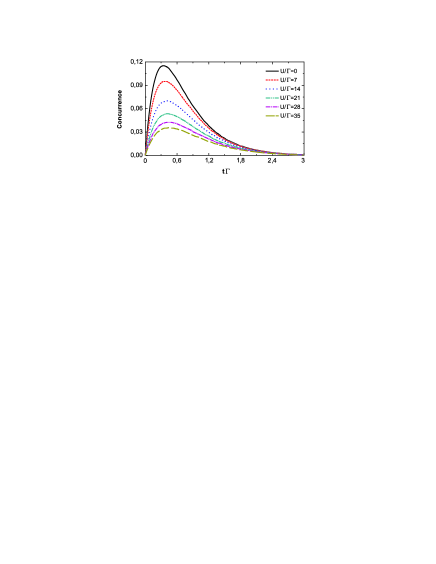
Figure 1: (Color online) Concurrence time evolution for different values of Coulomb interaction $U_{1}/\Gamma=U_{2}/\Gamma=U/\Gamma$. $\varepsilon_{1}/\Gamma=\varepsilon_{1}/\Gamma=7$, $T/\Gamma=2$, and $\Gamma=1$. Initial conditions are: $N_{S}(0)=0.5$, $N_{T}(0)=0.5$.

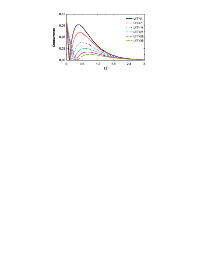
Figure 2: (Color online) Concurrence time evolution for different values of Coulomb interaction $U_{1}/\Gamma=U_{2}/\Gamma=U/\Gamma$. $\varepsilon_{1}/\Gamma=\varepsilon_{1}/\Gamma=7$, $T/\Gamma=2$, and $\Gamma=1$. Initial conditions are: $N_{S}(0)=0.55$, $N_{T}(0)=0.45$.

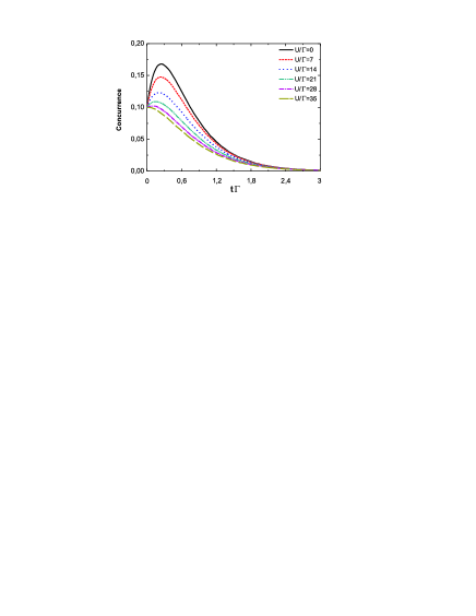
Figure 3: (Color online) Concurrence time evolution for different values of Coulomb interaction $U_{1}/\Gamma=U_{2}/\Gamma=U/\Gamma$. $\varepsilon_{1}/\Gamma=\varepsilon_{1}/\Gamma=7$, $T/\Gamma=2$, and $\Gamma=1$. Initial conditions are: $N_{S}(0)=0.45$, $N_{T}(0)=0.55$.

The behavior of time dependent quantum-dot system concurrence calculated by means of Eqs. (13), (25), (34) for different initial conditions is demonstrated in Figs.1-3. Figs.1, 2 demonstrate an important fact, that concurrence - the degree of entanglement, can increase during the relaxation processes in the system of coupled QDs, caused by the presence of on-site Coulomb correlations and interaction with the reservoir. Results depicted in Fig.3 reveal the possibility of system switching between entangled and unentangled (concurrence is equal to zero) states during the relaxation process.

II.3 Kinetic equations in pseudo-particle formalism

Another method of quantum-dot system dynamics analysis is based on the pseudo-particles formalism Coleman . Each pseudo-particle corresponds to particular eigenstate of the system. Transitions between the states with different number of electrons caused by coupling to reservoir can be analyzed in terms of pseudo-particle operators with constraint on the possible physical states (the number of pseudo-particles). Consequently, electron operator $c_{l\sigma}^{+}$ $(l=1,2)$ can be written in terms of pseudo-particle operators Maslova :

$$c_{l\sigma}^{+} = \sum_{i}X_{i}^{\sigma l}f_{i\sigma}^{+}b+\sum_{j,i}Y_{ji}^{\sigma-\sigma l}d_{j}^{+\sigma-\sigma}f_{i-\sigma}+$$

$$+ \sum_{i}Y_{i}^{\sigma\sigma l}d^{+\sigma\sigma}f_{i\sigma}+\sum_{m,j}Z_{mj}^{\sigma\sigma-\sigma l}\psi_{m-\sigma}^{+}d_{j}^{\sigma-\sigma}+$$

$$+ \sum_{m}Z_{m}^{\sigma-\sigma-\sigma l}\psi_{m\sigma}^{+}d^{-\sigma-\sigma}+\sum_{m}W_{m}^{\sigma-\sigma-\sigma l}\varphi^{+}\psi_{m\sigma}\$$

with constraint on the possible physical states

$$\widehat{n}_{b}+\sum_{i\sigma}\widehat{n}_{fi\sigma}+\sum_{j\sigma\sigma^{{}^{\prime}}}\widehat{n}_{dj}^{\sigma\sigma^{{}^{\prime}}}+\sum_{m\sigma}\widehat{n}_{\psi m\sigma}+\widehat{n}_{\varphi}=1,$$ (36)

where $f_{\sigma}^{+}(f_{\sigma})$ and $\psi_{\sigma}^{+}(\psi_{\sigma})$ - are pseudo-fermion creation (annihilation) operators for the electronic states with one and three electrons correspondingly. $b^{+}(b)$, $d_{\sigma}^{+}(d_{\sigma})$ and $\varphi^{+}(\varphi)$ - are slave boson operators, which correspond to the states without any electrons, with two electrons or four electrons. Operators $\psi_{m-\sigma}^{+}$ - describe system configuration with two spin up electrons $\sigma$ and one spin down electron $-\sigma$ in the symmetric and asymmetric states.

Further we’ll consider only single- and low energy double-occupied states, because the excited double-occupied states, three- and four- particle states are separated by the Coulomb gap. Consequently, all the terms containing $\varphi^{+}$ and $\psi_{m-\sigma}^{+}$ in expression (II.3) are omitted. Matrix elements $X_{i}^{\sigma l}$, $Y_{ji}^{\sigma-\sigma l}$ and $Y_{ji}^{\sigma\sigma l}$ can be defined as:

$$X_{i}^{\sigma l} = \langle\Psi_{i}^{\sigma}|c_{l\sigma}^{+}|0\rangle,$$

$$Y_{ji}^{\sigma-\sigma l} = \langle\Psi_{j}^{\sigma-\sigma}|c_{l\sigma}^{+}|\Psi_{i}^{-\sigma}\rangle,$$

$$Y_{ji}^{\sigma\sigma l} = \langle\Psi_{j}^{\sigma\sigma}|c_{l\sigma}^{+}|\Psi_{i}^{\sigma}\rangle.$$

So, taking into account constraint on the possible physical states the following non-stationary system of equations can be obtained for the pseudo-particle occupation numbers $N_{i}^{\sigma}$, $N_{j}^{\sigma-\sigma}$, $N_{j}^{\sigma\sigma}$ and $N_{b}$ by means of Heisenberg equations:

$$\frac{\partial N_{j}^{\sigma-\sigma}}{\partial t} = -2\Gamma\sum_{i\sigma}|Y_{ji}^{\sigma-\sigma}|^{2}\cdot N_{j}^{\sigma-\sigma},$$

$$\frac{\partial N_{i}^{\sigma}}{\partial t} = 2\Gamma\sum_{j}|Y_{ji}^{\sigma-\sigma}|^{2}N_{j}^{\sigma-\sigma}-$$

$$- 2\Gamma|X_{i}^{\sigma}|^{2}N_{i}^{\sigma}+2\Gamma\sum_{j}|Y_{ji}^{\sigma\sigma}|^{2}\cdot N_{j}^{\sigma\sigma},$$

$$\frac{\partial N_{b}}{\partial t} = 2\Gamma\sum_{i\sigma}|X_{i}^{\sigma}|^{2}\cdot N_{i}^{\sigma},$$

$$\frac{\partial N_{j}^{\sigma\sigma}}{\partial t} = -2\Gamma\sum_{i}|Y_{ji}^{\sigma\sigma}|^{2}\cdot N_{j}^{\sigma\sigma},$$ (38)

where matrix elements can be easily expressed through the elements of matrixes (6), (8) and (10) eigenvectors:

$$|X_{i}^{\sigma}|^{2} = |\nu_{i}+\mu_{i}|^{2},$$

$$|Y_{ji}^{\sigma-\sigma}|^{2} = |\alpha_{j}\mu_{i}+\beta_{j}\nu_{i}+\gamma_{j}\mu_{i}+\delta_{j}\nu_{i}|^{2},$$

$$|Y_{ji}^{\sigma\sigma}|^{2} = |\nu_{i}+\mu_{i}|^{2}.$$ (39)

Depending on the tunneling barrier width and height typical tunneling rate $\Gamma$ can vary from $10\mu eV$ Amaha to $1\div 5$ meVFransson . These equations conserve the total number of pseudo-particles:

$$N_{b}+\sum_{i\sigma}N_{i}^{\sigma}+\sum_{j\sigma\sigma^{{}^{\prime}}}N_{j}^{\sigma\sigma^{{}^{\prime}}}=const.$$ (40)

So, Eqs.(38) provide the fulfilment of constraint

$$N_{b}+\sum_{i\sigma}N_{i}^{\sigma}+\sum_{j\sigma\sigma^{{}^{\prime}}}N_{j}^{\sigma\sigma^{{}^{\prime}}}=1$$ (41)

during time evolution, if it occurs at the initial time moment.

System of Eqs.(38) can be solved analytically with initial conditions $N_{j}^{\sigma\sigma^{{}^{\prime}}}(0)=N_{j}$, $N_{a}^{\sigma}(0)=0$, $N_{s}^{\sigma}(0)=0$ and $N_{b}(0)=0$ ($\sum_{j}N_{j}=1$). For initial generally mixed singlet-triplet state (23):

$$N_{j}^{\sigma-\sigma}(t) = N_{j}\cdot e^{-2\lambda_{j}t},$$

$$N_{a}^{\sigma}(t) = \sum_{j}[\frac{\lambda_{ja}}{2\lambda_{j}-\lambda_{a}}\cdot(e^{-\lambda_{a}t}-e^{-2\lambda_{j}t})]\cdot N_{j},$$

$$N_{s}^{\sigma}(t) = \sum_{j}[\frac{\lambda_{js}}{2\lambda_{j}-\lambda_{s}}\cdot(e^{-\lambda_{s}t}-e^{-2\lambda_{j}t})]\cdot N_{j},$$

$$N_{b}(t) = 1-N_{dj}^{\sigma-\sigma}(t)-\sum_{\sigma}N_{a}^{\sigma}(t)-\sum_{\sigma}N_{s}^{\sigma}(t),$$

where

$$\lambda_{a(s)} = 2\Gamma\cdot|\mu_{a(s)}+\nu_{a(s)}|^{2},$$

$$\lambda_{ja(s)} = 2\Gamma\cdot|\alpha_{j}\mu_{a(s)}+\beta_{j}\nu_{a(s)}+\delta_{j}\nu_{a(s)}+\gamma_{j}\mu_{a(s)}|^{2},$$

$$\lambda_{j} = \sum_{i=a,s}\lambda_{ji}.$$ (43)

Electron occupation numbers $N_{el}$ can be determined through the pseudo-particle occupation numbers considering spin degrees of freedom by the following expression:

$$N_{el}(t)=\sum_{j}N_{j}\cdot[2e^{-2\lambda_{j}t}+2\sum_{i=a,s}\frac{\lambda_{ij}}{2\lambda_{j}-\lambda_{i}}(e^{-\lambda_{i}t}-e^{2\lambda_{j}t})].$$

According to concurrence definition through the eigenvalues of matrix $\widetilde{\rho}\rho$ for initial state (23):

$$C(t)=max(0,|N_{S^{0}}(t)-N_{T^{0}}(t)|),$$ (45)

where

$$N_{S^{0}}(t) = N_{S^{0}}(0)\cdot e^{-2\lambda_{S^{0}}t},$$

$$N_{T^{0}}(t) = N_{T^{0}}(0)\cdot e^{-2\lambda_{T^{0}}t},$$

$$\lambda_{S^{0}} = |\alpha+\beta|^{2}\cdot(\lambda_{s}+\lambda_{a}),$$

$$\lambda_{T^{0}} = \frac{1}{2}\cdot(\lambda_{s}+\lambda_{a}).$$ (46)

Concurrence time evolution for different initial conditions and values of Coulomb correlations is shown in Figs.1-3. Results obtained by both approaches exactly coincide for the same system parameters.

If at the initial time moment concurrence is not equal to zero [$C(0)\neq 0$] there can exist a time moment $t=t_{0}$, when concurrence turns to zero [$C(t_{0})=0$] (see Fig.2).

$$t_{0}=\frac{1}{2(\lambda_{S^{0}}-\lambda_{T^{0}})}\cdot ln(\frac{N_{S^{0}}}{N_{T^{0}}}).$$ (47)

Further system time evolution leads to the concurrence increasing reaching its maximum value

$$C(t_{max}) = N_{T^{0}}\cdot e^{\frac{-\lambda_{T^{0}}}{\lambda_{S^{0}}-\lambda_{T^{0}}}\cdot ln(\frac{N_{S^{0}}\cdot\lambda_{S^{0}}}{N_{T^{0}}\cdot\lambda_{T^{0}}})}-$$ (48)

$$- N_{S^{0}}\cdot e^{\frac{-\lambda_{S^{0}}}{\lambda_{S^{0}}-\lambda_{T^{0}}}\cdot ln(\frac{N_{S^{0}}\cdot\lambda_{S^{0}}}{N_{T^{0}}\cdot\lambda_{T^{0}}})}$$

at time moment

$$t_{max}=t_{0}+\frac{1}{2(\lambda_{S^{0}}-\lambda_{T^{0}})}\cdot ln(\frac{\lambda_{S^{0}}}{\lambda_{T^{0}}}).$$ (49)

So, concurrence could reveal non-monotonic behavior for mixed two-electronic initial state with opposite spins. We would like to mention that despite the fact that both theoretical approaches give the same result for the considered system of two coupled quantum dots with Coulomb correlations there is some difference between them. Theoretical approach based on the equations of motion for localized electrons occupation numbers (see Section A) provides possibility for the analysis of concurrence and spin correlations time dependent behavior in the complicated systems of many correlated coupled quantum dots taking into account all orders localized electron correlation functions and considering interference effects. A closed system of equations can be obtained for an arbitrary number of quantum dots in the situation of weak coupling to reservoir, but these equations will have a rather cumbersome form and can be hardly solved analytically. Theoretical approach based on the pseudo-particles formalism (see Section C) is more straightforward and provides the possibility to analyze analytically time evolution of the degree of entanglement in the system of quantum dots with a small number of available electronic states in the case of weak interaction between correlated quantum dots and reservoir. To conclude, both methods can be applied for the localized charge and spin kinetics analysis in coupled quantum dots with Coulomb correlations, but for the complicated systems method based on the equations of motion for localized electrons occupation numbers is more preferable. However, systems with a small number of available electronic states could be better analyzed by means of pseudo-particles formalism as it provides the possibility to obtain explicit expressions for the time evolution of system characteristics.

III Conclusion

Time evolution of initially prepared entangled state in the system of correlated coupled quantum dots has been analyzed by means of two different approaches. The first one is based on the equations of motion for all orders localized electron correlation functions taking into account interference effects. The second approach deals with the kinetic equations for pseudo-particle occupation numbers considering constraint on the possible physical states. Both approaches allow us to follow the changes of the entanglement during time evolution of the two coupled quantum dots system due to the concurrence direct link with quantum dots pair correlation functions. For different initial mixed states the concurrence (degree of entanglement) could reveal non-monotonic behavior and even considerably increase during the time evolution of quantum dots system. Obtained results reveal the possibility of system switching between entangled and unentangled (concurrence is equal to zero) states during the relaxation process. This fact provides the method of controllable tuning of the degree of entanglement for the electronic quantum dots systems based on the analysis of its non-stationary characteristics.

This work was supported by Russian Science Foundation (project no. $16-12-00072$). V.N.M. also acknowledge the support by the RFBR grant $16-32-60024$ $mol-a-dk$.

References

• (1) D. Loss, D.P. DiVincenzo, (Phys. Rev. A, 57, 120 (1998).
• (2) A. Imamoglu, D.D. Awschalom, G. Burkard, D.P. DiVincenzo, D. Loss, M. Sherwin, A. Small, (Phys. Rev. Lett., 83, 4204 (1999).
• (3) W. Yao, R.-B. Liu, L.J. Sham, (Phys. Rev. Lett., 95, 030504 (2005).
• (4) M. Blaauboer, D.P. DiVincenzo, (Phys. Rev. Lett., 95, 160402 (2005).
• (5) L. Robledo, J. Elzerman, G. Jundt, M. Atature, A. Hogele, S. Falt, A. Imamoglu, (Science, 320, 772 (2008).
• (6) K.C. Nowack, M. Shafiei, M. Laforest, G.E.D.K. Prawiroatmodjo, L.R. Schreiber, C. Reichl, W. Wegscheider, L.M.K. Vandersypen, (Science, 333, 1269 (2011).
• (7) M.D. Schulman, O.E. Dial, S.P. Harvey, H. Bluhm, V. Umansky, A. Yakobi, (Science, 336, 202 (2012).
• (8) N.S. Maslova, V.N. Mantsevich, P.I. Arseyev, (European Phys. J. B, 88, 40 (2015).
• (9) I. Bar-Joseph, S.A. Gurvitz, Phys.Rev B, 44, 3332, (1991).
• (10) S.A. Gurvitz, M.S. Marinov, Phys.Rev A, 40, 2166, (1989).
• (11) V.N. Mantsevich, N.S. Maslova, P.I. Arseyev, Solid State Comm., 152, 1545, (2012).
• (12) V.N. Mantsevich, N.S. Maslova,P.I. Arseyev, Solid State Comm., 168, 36, (2013).
• (13) P.I. Arseyev, N.S. Maslova, V.N. Mantsevich, JETP Lett., 95(10), 521, (2012).
• (14) C.A. Stafford, N.S. Wingreen, Phys. Rev. Lett., 76, 1916, (1996).
• (15) B.L. Hazelzet, M.R. Wegewijs, T. H. Stoof, Y.V. Nazarov, Phys. Rev. B, 63, 165313, (2001).
• (16) E. Cota, R. Aguado, G. Platero, Phys. Rev. Lett., 94, 107202, (2005).
• (17) P.I. Arseyev, N.S. Maslova, V.N. Mantsevich, JETP, 115(1), 141, (2012).
• (18) W.G. van der Wiel, Y.V. Nazarov, S. DeFranceschi, T. Fujisawa, J.M. Elzerman, E.W.G.M. Huizeling, S. Tarucha, L.P. Kouwenhoven, Phys. Rev. B, 67, 033307, (2003).
• (19) Y. Okazaki, S. Sasaki, K. Muraki, Phys. Rev. B, 84, 161305(R), (2011).
• (20) S. Amasha, A.J. Keller, I.G. Rau, A. Carmi, J.A. Katine, H. Shtrikman, Y. Oreg, D. Goldhaber-Gordon, Phys. Rev. Lett., 110, 046604, (2013).
• (21) M. Bayer, P. Hawrylak, K. Hinzer, S. Fafard, M. Korkusinski, Z.R. Wasilevski, O. Stern, A. Forchel, Science, 291, 451 (2001).
• (22) C. Creatore, R.T. Brierley, R.T. Phillips, P.B. Littlewood, P.R. Eastham, Phys. Rev. B, 86, 155442 (2012).
• (23) A.V. Tsukanov, Phys. Rev. A, 72, 022344 (2005).
• (24) N. Yokoshi, H. Imamura, H. Kosaka, Phys. Rev. B, 88, 155321 (2013)
• (25) G. Burkard, D. Loss, E.V. Sukhorukov, Phys. Rev. B, 61, R16303 (2000)
• (26) R. Sanchez, G. Platero, Phys. Rev. B, 87, 081305 (2013)
• (27) F. Cicarello, G. Palma, M. Zarcone, Y. Omar, V. Vicira, J. Phys. A, 40, 7993 (2007)
• (28) G. Burkard, D. Loss, D.P. DiVincenzo, Phys. Rev. B, 59, 2070 (1999)
• (29) C.A. Busser, F. Heidrich-Meisner, Phys. Rev. Lett., 111, 246807 (2013)
• (30) J.P. Dowling, G.J. Milburn, arXiv:quant-ph/0206091v1.
• (31) M.A. Nielsen, I.L. Chuang, Quantum Computation and Quantum Information, (Cambridge University Press, Cambridge, England, 2000).
• (32) R. Hanson, L.P. Kouwenhoven, J.R. Petta, S. Tarucha, L.M.K. Vandersypen, Rev. Mod. Phys., 79, 1217 (2007).
• (33) G.E. Murgida, D.A. Wisniacki, P.I. Tamborenea, Phys. Rev. Lett., 99, 036806 (2007).
• (34) M. Kataoka, M.R. Astley, A.L. Thorn, D.K.L. Oi, C.H.W. Barnes, C.J.B. Ford, D. Anderson, G.A.C. Jones, I. Farrer, D.A. Ritchie, and M. Pepper, Phys. Rev. Lett., 102, 156801 (2009).
• (35) A. Putaja, E. Rasanen, Phys. Rev. B, 82, 165336 (2010).
• (36) L. Saelen, R. Nepstad, I. Degani, J.P. Hansen, Phys. Rev. Lett., 100, 046805 (2008).
• (37) W.K. Wootters, Phys. Rev. Lett., 80, 2245 (1998)
• (38) Piers Coleman, Phys. Rev. B, 29, (1984), 3035.
• (39) S. Amaha, W. Izumida, T. Hatano, S. Teraoka, S. Tarucha, J. A. Gupta, and D. G. Austing, Phys. Rev. Lett., 110, (2013), 016803.
• (40) J. Fransson Phys. Rev. B, 69, 201304, (2004).