Learning to Warm-Start
Bayesian Hyperparameter Optimization

Abstract

Hyperparameter optimization aims to find the optimal hyperparameter configuration of a machine learning model, which provides the best performance on a validation dataset. Manual search usually leads to get stuck in a local hyperparameter configuration, and heavily depends on human intuition and experience. A simple alternative of manual search is random/grid search on a space of hyperparameters, which still undergoes extensive evaluations of validation errors in order to find its best configuration. Bayesian optimization that is a global optimization method for black-box functions is now popular for hyperparameter optimization, since it greatly reduces the number of validation error evaluations required, compared to random/grid search. Bayesian optimization generally finds the best hyperparameter configuration from random initialization without any prior knowledge. This motivates us to let Bayesian optimization start from the configurations that were successful on similar datasets, which are able to remarkably minimize the number of evaluations. In this paper, we propose deep metric learning to learn meta-features over datasets such that the similarity over them is effectively measured by Euclidean distance between their associated meta-features. To this end, we introduce a Siamese network composed of deep feature and meta-feature extractors, where deep feature extractor provides a semantic representation of each instance in a dataset and meta-feature extractor aggregates a set of deep features to encode a single representation over a dataset. Then, our learned meta-features are used to select a few datasets similar to the new dataset, so that hyperparameters in similar datasets are adopted as initializations to warm-start Bayesian hyperparameter optimization. Empirical experiments on various image datasets (i.e., AwA2, Caltech-101, Caltech-256, CIFAR-10, CIFAR-100, CUB-200-2011, MNIST, and VOC2012) demonstrate our meta-features are useful in optimizing hyperparameters of convolutional neural networks for an image classification task.

1 Introduction

Machine learning model ${{\mathcal{M}}}$ requires a choice of hyperparameter vector ${{\boldsymbol{\theta}}}$. This hyperparameter vector ${{\boldsymbol{\theta}}}$ is chosen in the Cartesian product space of hyperparameter vectors ${\boldsymbol{\Theta}}=\Theta_{1}\times\cdots\times\Theta_{d}$ where ${\boldsymbol{\theta}}=\left[\theta_{1},\ldots,\theta_{d}\right]^{\top}$ and ${\theta_{i}\in\Theta_{i}}$ for ${1\leq i\leq d}$. The vectors selected by machine learning experts using diverse experience and human intuition have guaranteed to find one of the best hyperparameter vectors which might show the best performance measure (e.g., classification error and mean squared error). However, such a naïve hyperparameter search is not enough to find the hyperparameter vector that shows the best performance, even though we utilized the experience and intuition. For this reason, many structured methods to find the better vector, such as random search, grid search (Bergstra and Bengio, 2012), improvement-based search (Kushner, 1964; Moćkus et al., 1978), and entropy search (Hennig and Schuler, 2012) have been proposed. In particular, various works (Hutter et al., 2011; Bergstra et al., 2011; Snoek et al., 2012; Kim et al., 2016) which repeat the following steps: (i) predicting function estimates and their uncertainty estimates by a surrogate function model ${{\mathcal{M}}_{\textrm{surrogate}}}$, (ii) evaluating domain space ${{\boldsymbol{\Theta}}}$ using outcomes of ${{\mathcal{M}}_{\textrm{surrogate}}}$, and (iii) acquiring a new vector ${{\boldsymbol{\theta}}^{\dagger}}$, have been employed into hyperparameter optimization.

To measure which vector will be the best hyperparameter vector, the space needs to be either exploited or explored. That trade-off of exploitation and exploration can be balanced by performance measure estimate and its uncertainty estimate, predicted by Bayesian regression models (e.g., Gaussian process regression (Jones et al., 1998) and Bayesian neural networks (Springenberg et al., 2016)). Such hyperparameter optimization that follows a framework of Bayesian optimization, referred to as Bayesian hyperparameter optimization (BHO) finds the vector to maximize an acquisition function ${a(\cdot)}$:

$${\boldsymbol{\theta}}^{\dagger}=\operatornamewithlimits{\arg\max}_{{\boldsymbol{\theta}}}a({\boldsymbol{\theta}}|\mathcal{M}_{\textrm{surrogate}}).$$

The details of BHO will be described in Section 2.1.

As summarized in Algorithm 1, ${k}$ initial vectors should be given in order to build a regression model. Generally, random sampling methods such as naïve uniform random sampling, Latin hypercube sampling (McKay et al., 1979), and quasi-Monte Carlo sampling are used to choose the initial vectors. However, from exploitation and exploration trade-off perspective, initial vectors should be selected carefully, since better initial hyperparameter vectors encourage BHO to prevent exploration and focus on exploitation. To find the better vectors, several works (Bonilla et al., 2008; Bardenet et al., 2013; Swersky et al., 2013; Yogatama and Mann, 2014) have proposed the methods to share and transfer prior knowledge using block covariance matrices. Moreover, hand-crafted and simply adjusted meta-features over datasets, measured by dataset similarity (Michie et al., 1994) have been proposed to transfer the prior knowledge to BHO (Pfahringer et al., 2000; Feurer et al., 2015; Wistuba et al., 2015). The details of related works are described in Section 3.

Algorithm 1 Bayesian Hyperparameter Optimization

1:Target function ${\mathcal{J}}(\cdot)$, $k$ initial hyperparameter vectors $\{{\boldsymbol{\theta}}_{1}^{\dagger},\ldots,{\boldsymbol{\theta}}_{k}^{\dagger}\}\subset{\boldsymbol{\Theta}}$, limit $T\in\mathbb{N}>k$

2:Best hyperparameter vector ${\boldsymbol{\theta}}^{\ast}\in{\boldsymbol{\Theta}}$

3:Initialize an acquired set as an empty set

4:for $i=1,2,\ldots,k$ do

5:     Evaluate ${\mathcal{J}}_{i}\coloneqq{\mathcal{J}}({\boldsymbol{\theta}}_{i}^{\dagger})$

6:     Accumulate $({\boldsymbol{\theta}}_{i}^{\dagger},{\mathcal{J}}_{i})$ into the acquired set

7:end for

8:for $j=k+1,k+2,\ldots,T$ do

9:     Estimate a surrogate function ${\mathcal{M}}_{\textrm{surrogate}}$ with the acquired set $\{({\boldsymbol{\theta}}_{i}^{\dagger},{\mathcal{J}}_{i})\}_{i=1}^{j-1}$

10:     Find ${\boldsymbol{\theta}}_{j}^{\dagger}=\operatornamewithlimits{\arg\max}_{{\boldsymbol{\theta}}}a(\boldsymbol{\theta}|\mathcal{M}_{\textrm{surrogate}})$

11:     Evaluate ${\mathcal{J}}_{j}\coloneqq{\mathcal{J}}({\boldsymbol{\theta}}_{j}^{\dagger})$

12:     Accumulate $({\boldsymbol{\theta}}_{j}^{\dagger},{\mathcal{J}}_{j})$ into the acquired set

13:end for

14:return ${\boldsymbol{\theta}}^{\ast}=\operatornamewithlimits{\arg\min}_{{\boldsymbol{\theta}}_{j}^{\dagger}\in\{{\boldsymbol{\theta}}_{1}^{\dagger},\ldots,{\boldsymbol{\theta}}_{T}^{\dagger}\}}\mathcal{J}_{j}$

In this paper, we propose the metric learning architecture to learn meta-features over datasets ${{\mathbf{m}}}$, and apply the learned meta-features in BHO. We train deep feature extractor and meta-feature extractor over datasets via Siamese network (Bromley et al., 1994), matching meta-feature distance function ${d_{\textrm{mf}}(\cdot,\cdot)}$ with target distance function ${d_{\textrm{target}}(\cdot,\cdot)}$ (see Section 2.2). After training the architecture, we determine $k$ datasets, comparing new test dataset with the datasets used in training the architecture. Finally, the configurations of $k$-nearest datasets, which are previously measured, are used to initialize BHO. To our best knowledge, this paper is the first work which proposes the method to warm-start BHO using the learned meta-features over datasets.

Before starting the main section, we summarize our contributions:

• we visualize the effects of hyperparameters and datasets with respect to performance measure in order to reveal why we need to learn a meta-feature,

• we introduce a meta-feature extractor, trained by historical prior knowledge from the subsampled datasets obtained from various image datasets (i.e., AwA2, Caltech-101, Caltech-256, CIFAR-10, CIFAR-100, CUB-200-2011, MNIST, and VOC2012),

• we initialize BHO with ${k}$-nearest datasets, which the learned meta-features of new dataset decide on, and find the best hyperparameter vector following BHO steps.

2 Background

In this section, we present Bayesian hyperparameter optimization and the reason why meta-features over datasets should be learned. In addition, we describe some definitions, distance matching and target distance, used to learn meta-features.

2.1 Bayesian Hyperparameter Optimization

Bayesian hyperparameter optimization (BHO), an application of Bayesian optimization (Brochu et al., 2010) searches the best hyperparameter vector on the domain space ${{\boldsymbol{\Theta}}}$. Suppose that we are given a dataset of training set and validation set ${\mathcal{D}}=\{{\mathcal{D}}_{\textrm{train}},{\mathcal{D}}_{\textrm{val}}\}$ with which we train a model involving hyperparameter vector ${{\boldsymbol{\theta}}}$. Given a dataset ${\mathcal{D}}$, the best hyperparameter vector is determined by minimizing the validation error ${\mathcal{J}}({\boldsymbol{\theta}},{\mathcal{D}}_{\textrm{train}},{\mathcal{D}}_{\textrm{val}})$. As described in Algorithm 1, inputs to BHO are: (i) a target function ${\mathcal{J}}({\boldsymbol{\theta}},{\mathcal{D}}_{\textrm{train}},{\mathcal{D}}_{\textrm{val}})$ (whose functional form is not known in most of cases) which returns validation error or classification performance given hyperparameter vector and training/validation datasets, (ii) $k$ different hyperparameter vectors at initial design $\{{\boldsymbol{\theta}}_{1}^{\dagger},\ldots,{\boldsymbol{\theta}}_{k}^{\dagger}\}$, and (iii) a limit $T$ which pre-specifies the number of candidates of hyperparameter vectors over which the best configuration is searched. Then, the BHO undergoes the procedures which are explained below to return the best configuration of hyperparameters ${\boldsymbol{\theta}}^{\ast}$.

The BHO searches a minimum, gradually accumulating $({\boldsymbol{\theta}}_{j}^{\dagger},{\mathcal{J}}({\boldsymbol{\theta}}_{j}^{\dagger}))$ with $j$ increasing. Starting with a set of initial design $\{({\boldsymbol{\theta}}_{1}^{\dagger},{\mathcal{J}}_{1}),\ldots,({\boldsymbol{\theta}}_{k}^{\dagger},{\mathcal{J}}_{k})\}$, a surrogate function model ${\mathcal{M}}_{\textrm{surrogate}}$ is fit with the accumulated set of hyperparameter vector and its corresponding validation error. In this paper, the Gaussian process (GP) regression model ${\mathcal{M}}_{\textrm{GP}}$ serves as a surrogate function which approximates the landscape of ${\mathcal{J}}$ over the space ${\boldsymbol{\Theta}}$. The surrogate function well approximates the regions exploited so far, but has high uncertainty about the regions which are not yet explored. Thus, rather than optimizing the surrogate function itself, the acquisition function $a({\boldsymbol{\theta}}|{\mathcal{M}}_{\textrm{GP}})$, which is constructed to balance a trade-off between exploitation and exploration, is optimized to select the next hyperparameter vector at which the validation error ${\mathcal{J}}$ is evaluated. Assuming that the current GP has posterior mean $\mu({\boldsymbol{\theta}})$ and posterior variance $\sigma^{2}({\boldsymbol{\theta}})$, two popular acquisition functions that we use in this paper are:

• expected improvement (EI) (Moćkus et al., 1978)

  $$a({\boldsymbol{\theta}}|\mathcal{M}_{\textrm{GP}}) =\mathbb{E}_{p\left(\mu\left({\boldsymbol{\theta}}\right)|{\boldsymbol{\theta}}\right)}\left[\max\{0,\mathcal{J}({\boldsymbol{\theta}}^{\ddagger})-\mu({\boldsymbol{\theta}})\}\right]$$

  $$=(\mathcal{J}({\boldsymbol{\theta}}^{\ddagger})-\mu({\boldsymbol{\theta}}))\Phi\left(z({\boldsymbol{\theta}})\right)+\sigma({\boldsymbol{\theta}})\phi\left(z({\boldsymbol{\theta}})\right),$$

  where ${z({\boldsymbol{\theta}})=(\mathcal{J}({\boldsymbol{\theta}}^{\ddagger})-\mu({\boldsymbol{\theta}}))/\sigma({\boldsymbol{\theta}})}$, ${\boldsymbol{\theta}}^{\ddagger}$ is the best point known thus far, $\Phi(\cdot)$ denotes the cumulative distribution function of the standard normal distribution, and $\phi(\cdot)$ represents the probability density function of the standard normal distribution,

• GP upper confidence bound (GP-UCB) (Srinivas et al., 2010)

  $$a({\boldsymbol{\theta}}|\mathcal{M}_{\textrm{GP}})=-\mu({\boldsymbol{\theta}})+\kappa\sigma({\boldsymbol{\theta}}),$$

  where $\kappa$ is a hyperparameter that balances exploitation and exploration to control the tightness of the confidence bounds.

2.2 Distance Matching and Target Distance for Metric Learning

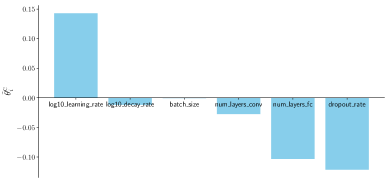
(a) Caltech-256 (90%)

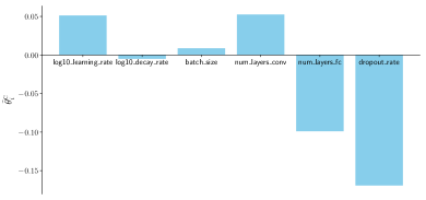
(b) CUB-200-2011 (80%)

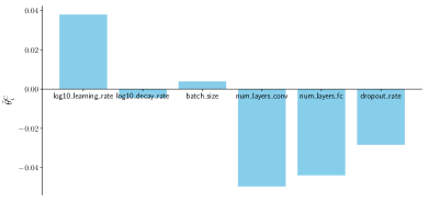
(c) MNIST (70%)

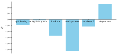
(d) VOC2012 (10%)

Figure 1: Subtracted CCoVs ${\tilde{\theta}_{i}^{c}}$ over hyperparameters for each dataset. ${i}$ in the subtracted CCoV indicates each hyperparameter dimension such as log10_learning_rate, log10_decay_rate, batch_size, num_layers_conv, num_layers_fc, and dropout_rate. Figures 1(a) to 1(d) show the subtracted CCoVs of each dataset. The details of datasets and hyperparameters are described in Section 5.1.

Meta-feature vector ${{\mathbf{m}}}$ produced by a meta-feature extractor ${{\mathcal{M}}_{\textrm{mf}}}$ is used to measure meta-feature distance, which is matched to a target distance. The model ${{\mathcal{M}}_{\textrm{mf}}}$ is learned by minimizing a residual of target distance function ${d_{\textrm{target}}(\cdot,\cdot)}$ and meta-feature distance function ${d_{\textrm{mf}}(\cdot,\cdot)}$:

$${\mathcal{M}}_{\textrm{mf}}^{\ast}=\operatornamewithlimits{\arg\min}_{{\mathcal{M}}_{\textrm{mf}}}\left\|d_{\textrm{target}}({\mathcal{D}}_{i},{\mathcal{D}}_{j})-d_{\textrm{mf}}\left(\mathbf{m}({\mathcal{D}}_{i}|{\mathcal{M}}_{\textrm{mf}}),{\mathbf{m}}({\mathcal{D}}_{j}|{\mathcal{M}}_{\textrm{mf}})\right)\right\|_{2}$$ (1)

where ${{\mathcal{D}}_{i}}$ and ${{\mathcal{D}}_{j}}$ denote datasets compared, defined in Section 2.1. ${{\mathcal{M}}_{\textrm{mf}}}$, which will be described in the subsequent section predicts the meta-feature vectors ${{\mathbf{m}}_{i}\coloneqq\mathbf{m}({\mathcal{D}}_{i}|{\mathcal{M}}_{\textrm{mf}})}$ and ${{\mathbf{m}}_{j}\coloneqq{\mathbf{m}}({\mathcal{D}}_{j}|{\mathcal{M}}_{\textrm{mf}})}$, which indicate the outputs of ${{\mathcal{M}}_{\textrm{mf}}}$ with respect to datasets ${{\mathcal{D}}_{i}}$ and ${{\mathcal{D}}_{j}}$, respectively.

Before introducing our deep meta-feature extractor ${{\mathcal{M}}_{\textrm{mf}}}$, we first explain how target distance is measured and why meta-feature distance function is effective. To measure target distance over datasets for metric learning, we need to collect prior knowledge from historical hyperparameter optimization. Assuming that there are ${\{({\boldsymbol{\theta}}_{s},{\mathcal{J}}_{s}^{(t)})\}_{s=1}^{n}}$ for ${1\leq t\leq K}$, where ${n}$ is the number of historical tuple of hyperparameter vector and validation error for each dataset, and ${K}$ is the number of the datasets which we have prior knowledge, we define a target distance function between two validation error vectors for the datasets ${{\mathcal{D}}_{i}}$ and ${{\mathcal{D}}_{j}}$, defined as ${L_{1}}$ distance:

$$d_{\textrm{target}}({\mathcal{D}}_{i},{\mathcal{D}}_{j}) =\left\|\left[{\mathcal{J}}_{1}^{(i)}\cdots{\mathcal{J}}_{n}^{(i)}\right]-\left[{\mathcal{J}}_{1}^{(j)}\cdots{\mathcal{J}}_{n}^{(j)}\right]\right\|_{1}$$

$$=\sum_{s=1}^{n}|{\mathcal{J}}_{s}^{(i)}-{\mathcal{J}}_{s}^{(j)}|$$ (2)

where ${1\leq i,j\leq K}$.

The target distance function, computed by historical validation errors, represents how different two datasets are. For this implication, we can understand the target distance (computed by Equation 2) as the ground-truth pairwise distance. However, there are two reasons why the target distance cannot be employed as the ground-truth distance directly: (i) a distance for new dataset without prior knowledge cannot be measured, and (ii) a distance function, which can be interpreted as a mapping from hyperparameter space to validation error has a different multi-modal distribution with other mappings for different datasets. The first reason is truly obvious, but we do not know yet whether or not a mapping from hyperparameter space to the error over datasets is multi-modal.

Since the dimension of hyperparameter space is higher than three-dimensional space, the mapping is difficult to visualize. Thus, instead of visualizing directly, we adapt a concept of center of mass. We compute a coordinate of center of validation error (CCoV) ${\theta_{i}^{\textrm{c}}}$ for a dimension $i$:

$$\theta^{\textrm{c}}_{i}=\frac{\sum_{s=1}^{n}{\tilde{\theta}}_{si}{\mathcal{J}}_{s}}{\sum_{s=1}^{n}{{\mathcal{J}}}_{s}}$$ (3)

where a normalized hyperparameter

$${\tilde{\theta}}_{si}=\frac{\theta_{si}-\min_{s=1,\dots,n}\theta_{si}}{\max_{s=1,\dots,n}\theta_{si}-\min_{s=1,\dots,n}\theta_{si}}$$

for ${1\leq i\leq d}$ is provided. Note that the superscript of ${{\mathcal{J}}_{s}^{(i)}}$ in Equation 2 are dropped to simplify Equation 3. Because Equation 3 individually represents one dataset, it can be dropped. As shown in Figure 1, each hyperparameter has different CCoV and those trends for each dataset are also different. It implies that locations of modes are different over datasets. To show the differences for all dimensions ${1\leq i\leq d}$ clearly, we subtract ${0.5}$ from CCoV:

$${\tilde{\theta}}_{i}^{\textrm{c}}=\theta_{i}^{\textrm{c}}-0.5.$$

Given the subtracted CCoV ${\tilde{\theta}_{i}^{\textrm{c}}}$ such as Figure 1, the cases of which ${\tilde{\theta}_{i}^{\textrm{c}}}$ is larger than zero imply mode might be located in the region which has large absolute value (e.g., log10_learning_rate in Figures 1(a) to 1(c)). If the original domain (e.g., log10_learning_rate and log10_decay_rate, see Table 2) is negative, that means the location of mode is on the region which has small value. On the other hand, if ${\tilde{\theta}_{i}^{\textrm{c}}}$ is smaller than zero, it implies mode might be located in the region that has small absolute value (e.g., num_layers_conv in Figures 1(c) and 1(d) and num_layers_fc in Figures 1(a) to 1(d)). As shown in Figure 1, some trends of ${\tilde{\theta}_{i}^{\textrm{c}}}$ are different over datasets. Furthermore, there are the cases which have different plus or negative sign (i.e., log10_learning_rate, num_layers_conv, and dropout_rate). Finally, based on these observations, we can argue the mappings from hyperparameter space to validation error have multi-modal distributions over datasets.

3 Related Work

Hyperparameter optimization based on grid search or random search has been proposed (Bergstra and Bengio, 2012). Recently, various hyperparameter optimization methods based on Bayesian optimization or sequential model-based optimization have been proposed, and they demonstrate that Bayesian optimization or sequential model-based optimization performs better than grid search and random search with a small number of evaluations of validation error. Hutter et al. (2011) suggest sequential model-based algorithm configuration method that models surrogate function as random forests. Snoek et al. (2012) propose the integrated acquisition function, computed by Markov chain Monte Carlo estimation over acquisition functions varied by hyperparameters of GP regression. Bergstra et al. (2011) present Bayesian optimization which uses tree-structured Parzen estimator as a surrogate function modeling method.

Also, several works to meta-learn, transfer, or warm-start Bayesian optimization have been proposed. A meta-learning (Schmidhuber, 1987; Thrun and Pratt, 1998) method for Bayesian optimization is recently proposed (Chen et al., 2017). Some works (Bonilla et al., 2008; Bardenet et al., 2013; Swersky et al., 2013; Yogatama and Mann, 2014; Poloczek et al., 2016) capture and transfer the shared information between tasks using covariance functions in the context of GP regression. In addition, the dataset similarity introduced in the literature (Michie et al., 1994) is used in transferring a prior knowledge to BHO (Pfahringer et al., 2000; Feurer et al., 2015; Wistuba et al., 2015). However, most of works, especially the methods based on the dataset similarity (Pfahringer et al., 2000; Feurer et al., 2015; Wistuba et al., 2015) are not suitable to measure similarity between image datasets, because they measure the similarity with respect to hand-crafted statistics and simply learned landmark information.

From now on, we introduce the works related to our Siamese network with meta-feature extractors. Various models with Siamese architecture, including CNNs (Bromley et al., 1994), MLPs (Chen and Salman, 2011) and RNNs (Mueller and Thyagarajan, 2016), have been developed for deep metric learning since its first appearance in the work (Bromley et al., 1994). All models have identical wings which extract meaningful features, and they are used to measure a distance between the inputs of wings.

Since in this paper we use two designs as a wing of Siamese network: (i) feature aggregation and (ii) bi-directional long short-term memory network (LSTM) (see Section 4), we attend to two structure of which the inputs are a set. Feature aggregation method appeared in several works (Edwards and Storkey, 2016; Qi et al., 2017; Zaheer et al., 2017) takes a linear combination of feature vectors derived from instances in a set, and bi-directional LSTM for a set (Vinyals et al., 2016) is also proposed. They argue the tasks which take a set can be learned using such structures. Moreover, Zaheer et al. (2017) show that aggregation of feature vectors transformed by instances is invariant to the permutation of instances in a set.

4 Proposed Model

We introduce our architecture composed of Siamese networks with deep feature and meta-feature extractors, as shown in Figure 2. Our network generates a deep feature of each instance in the dataset, and a set of deep features are fed into the meta-feature extractor to generate a meta-feature of dataset.

4.1 Overall Structure of Siamese Network

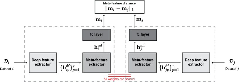
Figure 2: An illustration to show our Siamese network with deep feature extractor and meta-feature extractor. Deep feature extractor produces ${\{\mathbf{h}_{ip}^{\textrm{df}}\}_{p=1}^{\tau}}$ and ${\{\mathbf{h}_{jp}^{\textrm{df}}\}_{p=1}^{\tau}}$ for datasets ${{\mathcal{D}}_{i}}$ and ${{\mathcal{D}}_{j}}$, respectively. Next, meta-feature extractor produces ${\mathbf{h}_{i}^{\textrm{mf}}}$ and ${\mathbf{h}_{j}^{\textrm{mf}}}$, and the hindmost fully-connected layer (denoted as fc layer) produces ${\mathbf{m}_{i}}$ and ${\mathbf{m}_{j}}$. All shared weights are updated via minimizing the difference between meta-feature distance and target distance.

Algorithm 2 Learning a Siamese Network over Datasets

1:A set of $n$ datasets ${\{{\mathcal{D}}_{1},\ldots,{\mathcal{D}}_{n}\}}$, target distance function ${d_{\textrm{target}}(\cdot,\cdot)}$, number of subsamples in a dataset ${\tau\in\mathbb{N}}$, number of iterations $T\in\mathbb{N}$

2:Deep feature extractor and meta-feature extractor (${{\mathcal{M}}_{\textrm{df}}}$, ${{\mathcal{M}}_{\textrm{mf}}}$) trained over ${\{{\mathcal{D}}_{1},\ldots,{\mathcal{D}}_{n}\}}$

3:Initialize ${{\mathcal{M}}_{\textrm{df}}}$ and ${{\mathcal{M}}_{\textrm{mf}}}$

4:for $t=1,2,\ldots,T$ do

5:     Sample a pair of datasets, i.e., $({\mathcal{D}}_{i},{\mathcal{D}}_{j})$ for ${i\neq j}$, ${i,j=1,\ldots,n}$

6:     Sample $\tau$ instances from each dataset in the pair $({\mathcal{D}}_{i},{\mathcal{D}}_{j})$ selected above, to make ${|{\mathcal{D}}_{i}|=|{\mathcal{D}}_{j}|=\tau}$

7:     Update weights in ${\mathcal{M}}_{\textrm{df}}$ and ${\mathcal{M}}_{\textrm{mf}}$ using ${d_{\textrm{target}}({\mathcal{D}}_{i},{\mathcal{D}}_{j})}$ via optimizing Equation 1

8:end for

9:return $({\mathcal{M}}_{\textrm{df}},{\mathcal{M}}_{\textrm{mf}})$

A Siamese network is used to learn a metric such that distance between meta-features of datasets is well matched to the target distance. Our Siamese network has two identical wings each of which is composed of deep feature and meta-feature extractors (denoted as ${\mathcal{M}}_{\textrm{df}}$ and ${\mathcal{M}}_{\textrm{mf}}$, respectively). Specifically, the deep feature extractor transforms an instance of ${\mathcal{D}}_{i}$ into ${\mathbf{h}}^{\textrm{df}}_{ip}$ for $p=1,\ldots,n_{i}$, where $n_{i}$ is the number of instances in the dataset ${{\mathcal{D}}_{i}}$. The meta-feature extractor transforms a set of deep features $\{{\mathbf{h}}^{\textrm{df}}_{ip}\}_{p=1}^{n_{i}}$ into a meta-feature of ${\mathcal{D}}_{i}$, denoted as ${\mathbf{m}}_{i}$.

Learning the proposed network requires the following inputs: (i) a set of ${n}$ datasets ${\{{\mathcal{D}}_{1},\ldots,{\mathcal{D}}_{n}\}}$, (ii) target distance function ${d_{\textrm{target}}(\cdot,\cdot)}$, (iii) the number of samples ${\tau}$ in a dataset, and (iv) the iteration number ${T}$. Algorithm 2 shows the procedure where deep feature and meta-feature extractors are iteratively trained by minimizing Equation 1. Specifically, we follow three steps in the iteration: (i) a pair of datasets is sampled from a collection of datasets (see Section 5.1), (ii) ${\tau}$ instances are sampled from each dataset in the pair, and (iii) weights in ${\mathcal{M}}_{\textrm{df}}$ and ${{\mathcal{M}}_{\textrm{mf}}}$ are updated via optimizing Equation 1.

Large $\tau$ (e.g., ${\tau\coloneqq n_{i}}$) makes learning procedure unstable and diverged. However, simultaneously learning the networks with small $\tau$ seems to be converged to a local solution that poorly generalizes unseen instances. Therefore, Algorithm 2 should be expanded to the mini-batch version that updates weights via mini-batch gradient descent. The mini-batch version collects a set of ${\tau}$ instances by repeating Line 4 of Algorithm 2, and updates weights via mini-batch gradient descent.

4.2 Meta-Feature Extractor

Before explaining the details of meta-feature extractors, we first introduce the issues about handling instances of datasets. Dataset is a set of instances (i.e., images in this paper) which is invariant to the order of instances and varies the number of instances for each dataset. Therefore, it is difficult to feed in deep neural networks as well as common shallow classifiers, which have fixed input size. To resolve these problems, we consider two designs into meta-feature extractor:

• aggregation of deep features (ADF): deep features ${{\mathbf{h}}^{\textrm{df}}}$, derived from deep neural networks (e.g., convolutional layers and fully-connected layers) are aggregated as summation or arithmetic mean of them:

  $${\mathbf{h}}^{\textrm{mf}}\coloneqq{\mathbf{h}}_{\textrm{ADF}}=\sum_{p=1}^{\tau}{\mathbf{h}}^{\textrm{df}}_{p}\quad\textrm{or}\quad\frac{1}{\tau}\sum_{p=1}^{\tau}{\mathbf{h}}^{\textrm{df}}_{p},$$

• bi-directional long short-term memory network (Bi-LSTM): the deep features ${{\mathbf{h}}^{\textrm{df}}}$ are fed into Bi-LSTM. Bi-LSTM can be written as

  $${\mathbf{h}}^{\textrm{mf}}\coloneqq{\mathbf{h}}_{\textrm{Bi-LSTM}}=\textrm{Bi-LSTM}({\mathbf{h}}^{\textrm{df}}_{1:\tau}),$$

  where ${{\mathbf{h}}^{\textrm{df}}_{1:\tau}}$ denotes ${[{\mathbf{h}}^{\textrm{df}}_{1},{\mathbf{h}}^{\textrm{df}}_{2},\ldots,{\mathbf{h}}^{\textrm{df}}_{\tau-1},{\mathbf{h}}^{\textrm{df}}_{\tau}]}$.

As we mentioned in Section 3, they do not depend on the number of instances, and also they tend not to be affected by the order of instances. In order to learn a meaningful weights of meta-feature extractor, we input deep features ${{\mathbf{h}}^{\textrm{df}}}$ into meta-feature extractor (e.g., ADF or Bi-LSTM). The deep features obtained after passing convolutional and fully-connected layers with non-linear activation function can be used. Finally, fully-connected layer, followed by the output of meta-feature extractor produces a meta-feature vector, as shown in Figure 2. The details and practical configuration of meta-feature extractors will be described in the subsequent section.

5 Experiments

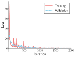
(a) ADF

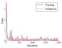
(b) Bi-LSTM

Figure 3: Training and validation losses of ADF and Bi-LSTM for 2,000 iterations.

We conducted experiments on learning our models and warm-starting BHO with the following experiment setups. In the end of this section, we will show learned meta-features are helpful to initialize BHO, as shown in Figure 4.

5.1 Experiment Setup

5.1.1 Collection of Datasets Processing

We created a collection of datasets for training our model, using eight image datasets:

1. Animals with Attributes 2 (AwA2) (Xian et al., 2017): 37,322 images of 50 classes,

2. Caltech-101: 9,146 images of 101 classes,

3. Caltech-256 (Griffin et al., 2007): 30,607 images of 256 classes,

4. CIFAR-10: 50,000 training images and 10,000 test images of 10 classes,

5. CIFAR-100: 50,000 training images and 10,000 test images of 100 classes,

6. Caltech-UCSD Birds-200-2011 (CUB-200-2011) (Wah et al., 2011): 11,788 images of 200 classes,

7. MNIST: 60,000 training images and 10,000 test images of 10 classes,

8. PASCAL Visual Objective Classes Challenge 2012 (VOC2012) (Everingham et al., 2012): 5,717 training images and 5,823 test images of 20 classes. Since VOC2012 is a multi-label dataset, we randomly select one of true labels.

We split each dataset to training, validation and test datasets. We trained a target model (see the subsequent section) using training datasets, and validation datasets are used to measure validation errors for the target model. Hyperparameter vectors and their validation errors measured by the trained target model are used to train our deep feature and meta-feature extractors. Moreover, test datasets are considered as new datasets.

If a dataset has a test dataset, we kept it and split training dataset to training and validation datasets. On the contrary, if a dataset does not include a test dataset, we split the dataset to training, validation, and test datasets. To magnify the datasets and vary ${\tilde{\theta}_{i}^{\textrm{c}}}$, we subsampled stratified ${\{10\%}$, ${20\%}$, ${\ldots}$, ${90\%}$, ${100\%\}}$ portions of original datasets from the training datasets. In this paper, we had a collection of 80 datasets, 10 subsampled datasets of 8 image datasets.

5.1.2 Target Model Setup

Table 1: Explanation and range of six-dimensional hyperparameter space. Each space ${\Theta}$ is closed-interval real number space or set. Especially, because a large number of elements in the set cause to generate high-dimensional space internally, batch_size is on the real number space. To convert a real number to integer, batch_size is wrapped by integer casting function when the selected hyperparameters are set up to the target model in practice.

Hyperparameter	Explanation	Range	Type
log10_learning_rate	${\log_{10}}$-scaled initial learning rate	${[-5.0,0.0]}$	Real
log10_decay_rate	${\log_{10}}$-scaled exponential decay	${[-8.0,-4.0]}$	Real
	for learning rate
batch_size	batch size	${[100,400]}$	Real
	(wrapped by integer casting)		(casted to Integer)
num_layers_conv	# of convolutional layers	${\{1,2,\ldots,9\}}$	Integer
num_layers_fc	# of fully-connected layers	${\{1,2,3\}}$	Integer
dropout_rate	dropout rate for dropout layer	${[0.0,0.9]}$	Real

Table 2: Detailed designs of feature extractor and meta-feature extractor. ADF and Bi-LSTM have the following structures. Output channels of convolutional layer, output dimensions of fully-connected layer, and hidden node size of Bi-LSTM are described in parentheses.

	Aggregation of deep features	Bi-directional LSTM
Deep feature extractor	3 ${\times}$ convolutional layer with ReLU (32, 64, 32 channels)
	-	fully-connected layer with ReLU
		(128 dims)
	flattening (+ labels)
Meta-feature extractor	Arithmetic mean aggregation	Bi-LSTM (128 dims)
After extractors	2 ${\times}$ fully-connected layer with ReLU (256, 256 dims)
	fully-connected layer (256 dims)

In this paper we optimized and warm-started convolutional neural network (CNN), created by six-dimensional hyperparameter vector ${(\textsf{log10\_learning\_rate},}$ ${\textsf{log10\_decay\_rate},}$ ${\textsf{batch\_size},}$ ${\textsf{num\_layers\_conv},}$ ${\textsf{num\_layers\_fc},}$ ${\textsf{dropout\_rate})}$, as shown in Table 1. Assuming that we are given the number of convolutional and fully-connected layers, num_layers_conv and num_layers_fc, we construct CNN with initial number 32 of ${3\times 3}$ convolutional filters, max-pooling layers with ${2\times 2}$ filters, and the fixed node number 256 of fully-connected layers. The number of convolutional filters are automatically increased and decreased. For example, if we have five convolutional layers, the number of the filters is ${(32,64,128,64,32)}$. All convolutional layers have batch normalization and dropout layer with dropout_rate is applied in fully-connected layers. CNN is trained by Adam optimizer with given batch_size and learning rate. We scheduled learning rate with exponential decay policy: ${l=10^{l_{0}}\exp(-10^{\eta}t)}$, where ${l_{0}}$ is log10_learning_rate, ${\eta}$ is log10_decay_rate, and ${t}$ is the iteration number.

5.1.3 Feature Extractors Setup

Algorithm 3 Bayesian Hyperparameter Optimization with Warm-Starting

1:Learned deep feature and meta-feature extractors ${({\mathcal{M}}_{\textrm{df}},{\mathcal{M}}_{\textrm{mf}})}$, target function ${\mathcal{J}}(\cdot)$, limit $T\in\mathbb{N}$, number of initial vectors $k<T$

2:Best hyperparameter vector ${\boldsymbol{\theta}}^{\ast}$

3:Find ${k}$-nearest neighbors using the learned deep feature and meta-feature extractors, ${({\mathcal{M}}_{\textrm{df}},{\mathcal{M}}_{\textrm{mf}})}$

4:Obtain ${k}$ historical sets of tuples ${\{\{({\boldsymbol{\theta}}_{s},{\mathcal{J}}_{s}^{(1)})\}_{s=1}^{n},\ldots,\{({\boldsymbol{\theta}}_{s},{\mathcal{J}}_{s}^{(k)})\}_{s=1}^{n}\}}$

5:Initialize an acquired set as an empty set

6:for $i=1,2,\ldots,k$ do

7:     Find the best vector ${{\boldsymbol{\theta}}_{i}^{\dagger}}$ on grid of the ${i}$-th set of tuples ${\{({\boldsymbol{\theta}}_{s},{\mathcal{J}}_{s}^{(i)})\}_{s=1}^{n}}$

8:     Evaluate ${\mathcal{J}}_{i}\coloneqq{\mathcal{J}}({\boldsymbol{\theta}}_{i}^{\dagger})$

9:     Accumulate $({\boldsymbol{\theta}}_{i}^{\dagger},{\mathcal{J}}_{i})$ into the acquired set

10:end for

11:for $j=k+1,k+2,\ldots,T$ do

12:     Estimate a surrogate function ${\mathcal{M}}_{\textrm{surrogate}}$ with the acquired set $\{({\boldsymbol{\theta}}_{i}^{\dagger},{\mathcal{J}}_{i})\}_{i=1}^{j-1}$

13:     Find ${\boldsymbol{\theta}}_{j}^{\dagger}=\operatornamewithlimits{\arg\max}_{{\boldsymbol{\theta}}}a({\boldsymbol{\theta}}|{\mathcal{M}}_{\textrm{surrogate}})$.

14:     Evaluate ${\mathcal{J}}_{j}\coloneqq{\mathcal{J}}({\boldsymbol{\theta}}_{j}^{\dagger})$

15:     Accumulate $({\boldsymbol{\theta}}_{j}^{\dagger},{\mathcal{J}}_{j})$ into the acquired set

16:end for

17:return ${\boldsymbol{\theta}}^{\ast}=\operatornamewithlimits{\arg\min}_{{\boldsymbol{\theta}}_{j}^{\dagger}\in\{{\boldsymbol{\theta}}_{1}^{\dagger},\ldots,{\boldsymbol{\theta}}_{T}^{\dagger}\}}{\mathcal{J}}_{j}$

To learn a distance function using Siamese network, the network composed of deep feature extractor and meta-feature extractor are used as a wing of Siamese network. As shown in Table 2, ADF has three convolutional layers with ReLU as deep feature extractor and arithmetic mean aggregation as meta-feature extractor, and Bi-LSTM has three convolutional layers with ReLU, which follows fully-connected layer with ReLU as deep feature extractor and Bi-LSTM as meta-feature extractor. Inputs of both ADF and Bi-LSTM have additional dimension for label information as well as the outputs of deep feature extractors, in order to feed useful information which is available to the meta-feature extractor. And also, they follow two fully-connected layers with ReLU and one fully-connected layer. As a result, the last output of the last fully-connected layer is used as meta-feature vector.

5.1.4 Bayesian Optimization Setup

We employed Bayesian optimization package, GPyOpt (The GPyOpt authors, 2016) in BHO. GP regression with automatic relevance determination (ARD) Matérn 5/2 kernel is used as surrogate function, and EI and GP-UCB are used as acquisition functions. All experiments are repeated five times.

5.2 Siamese Network Training

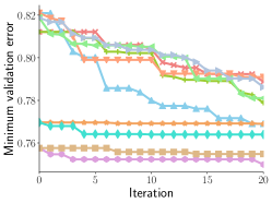
(a) AwA2

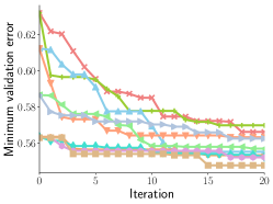
(b) Caltech-101

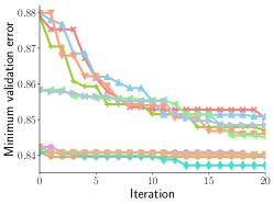
(c) Caltech-256

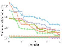
(d) CIFAR-10

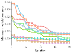
(e) CIFAR-100

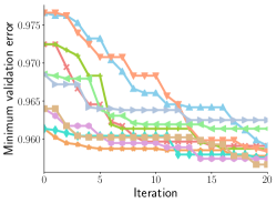
(f) CUB-200-2011

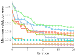
(g) MNIST

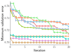
(h) VOC2012

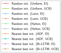
Figure 4: BHO for eight test datasets: AwA2, Caltech-101, Caltech-256, CIFAR-10, CIFAR-100, CUB-200-2011, MNIST, and VOC2012. Uniform, Latin, and Halton stand for näive uniform random sampling, Latin hypercube sampling, and quasi-Monte Carlo sampling with Halton sequence, respectively. Standard deviations are not depicted for clarity of figures.

We trained Siamese networks with ADF and Siamese networks with Bi-LSTM, the structures of which are defined in Table 2. They are optimized with Adam optimizer with the number of subsamples 200 and the exponentially decaying learning rate, which has initial learning rate ${10^{-4}}$ and exponential decay rate of learning rate ${10^{-3}}$.

Figure 3 shows validation loss as well as training loss are converged to almost zero, and it means our networks can be trained and meta-feature extractor produces an appropriate meta-feature vector that has small loss between target distance and meta-feature distance (see the argument for ${\operatornamewithlimits{\arg\min}}$ in Equation 1). Learned meta-feature extractor is used in Section 5.3.

5.3 Bayesian Hyperparameter Optimization with Warm-Starting

The learned meta-feature extractor which is trained by Algorithm 2 is employed in BHO. BHO with warm-starting, described in Algorithm 3 has inputs: (i) learned deep feature and meta-feature extractors ${({\mathcal{M}}_{\textrm{df}},{\mathcal{M}}_{\textrm{mf}})}$, (ii) target function ${{\mathcal{J}}(\cdot)}$, (iii) limit ${T}$, and (iv) the number of initial vectors ${k<T}$. It follows the similar steps (Lines 9 to 14 of Algorithm 3) in Algorithm 1, but initialization steps (Lines 1 to 8 of Algorithm 3) is different. Thus, in this section we focus on the initialization step.

As shown in Line 1 of Algorithm 3, we find ${k}$-nearest datasets using the meta-feature vectors derived from ${({\mathcal{M}}_{\textrm{df}},{\mathcal{M}}_{\textrm{mf}})}$. More precisely, we compute the meta-feature vector of new dataset ${{\mathbf{m}}_{\textrm{new}}}$ as well as the meta-feature of the datasets in a collection of datasets ${\{{\mathbf{m}}_{c}\}_{c=1}^{\gamma}}$ where ${\gamma}$ is the number of datasets in the collection of datasets. As mentioned in Section 5.1, ${\gamma=80}$ in this paper. Comparing ${{\mathbf{m}}_{\textrm{new}}}$ to ${\{{\mathbf{m}}_{c}\}_{c=1}^{\gamma}}$, we can find ${k}$-nearest datasets. For ${k}$-nearest datasets, we can select the best hyperparameter vector of dataset ${{\mathcal{D}}_{i}}$ from the historical tuple ${\{({\boldsymbol{\theta}}_{s},{\mathcal{J}}_{s}^{(i)})\}_{s=1}^{n}}$ for all ${1\leq i\leq k}$. Those ${k}$ initial hyperparameter vectors are used to initialize BHO. In this paper, we used ${3}$ initial hyperparameter vectors for all experiments.

As shown in Figure 4, we conducted 10 experiments for each test dataset. To compare our two methods: 3-nearest best vector initialization predicted by ADF and Bi-LSTM, we used three initialization techniques: (i) naïve uniform random sampling (denoted as uniform), (ii) Latin hypercube sampling (denoted as Latin), (iii) quasi-Monte Carlo sampling with one of low discrepancy sequences, Halton sequence (denoted as Halton). Moreover, we tested two acquisition functions: EI and GP-UCB (denoted as UCB) for five initialization methods.

The compared initialization methods are widely used in initializing BHO. In particular, because naïve uniform sampling leads to overlapped sampling for each dimension, Latin hypercube sampling and quasi-Monte Carlo sampling are often used. Two methods sample random vectors that have low overlapped region for each dimension, and they are effective in sampling on high-dimensional space.

All experiments show our methods perform better than other initialization methods. In addition, Bi-LSTM shows better performance than ADF in most of the experiments. It implies that Bi-LSTM can learn and extract meta-features well, rather than ADF.

6 Conclusion

In this paper we learned meta-feature over datasets using Siamese network with deep feature extractor and meta-feature extractor, in order to warm-start BHO. We considered identical wings of Siamese network as either ADF or Bi-LSTM, and each design shows the network can match pairwise meta-feature distance over datasets with pairwise target distance over them. Finally, the learned meta-features are used to find a few nearest datasets, and their historical best hyperparameter vectors are utilized in initializing BHO. Our experiment results for CNNs created by six-dimensional hyperparameter vectors demonstrate that learned meta-features are effective to warm-start BHO.

References

- Bardenet et al. [2013] R. Bardenet, M. Brendel, B. Kégl, and M. Sebag. Collaborative hyperparameter tuning. In Proceedings of the International Conference on Machine Learning (ICML), pages 199–207, Atlanta, Georgia, USA, 2013.
- Bergstra and Bengio [2012] J. Bergstra and Y. Bengio. Random search for hyper-parameter optimization. Journal of Machine Learning Research, 13:281–305, 2012.
- Bergstra et al. [2011] J. Bergstra, R. Bardenet, Y. Bengio, and B. Kégl. Algorithms for hyper-parameter optimization. In Advances in Neural Information Processing Systems (NIPS), volume 24, pages 2546–2554, Granada, Spain, 2011.
- Bonilla et al. [2008] E. V. Bonilla, K. M. A. Chai, and C. K. I. Williams. Multi-task Gaussian process prediction. In Advances in Neural Information Processing Systems (NIPS), volume 21, pages 153–160, Vancouver, British Columbia, Canada, 2008.
- Brochu et al. [2010] E. Brochu, V. M. Cora, and N. de Freitas. A tutorial on Bayesian optimization of expensive cost functions, with application to active user modeling and hierarchical reinforcement learning. arXiv preprint arXiv:1012.2599, 2010.
- Bromley et al. [1994] J. Bromley, I. Guyon, Y. LeCun, E. Säckinger, and R. Shah. Signature verification using a “Siamese” time delay neural network. In Advances in Neural Information Processing Systems (NIPS), volume 7, pages 737–744, Denver, Colorado, USA, 1994.
- Chen and Salman [2011] K. Chen and A. Salman. Extracting speaker-specific information with a regularized Siamese deep network. In Advances in Neural Information Processing Systems (NIPS), volume 24, pages 298–306, Granada, Spain, 2011.
- Chen et al. [2017] Y. Chen, M. W. Hoffman, S. G. Colmenarejo, M. Denil, T. P. Lillicrap, M. Botvinick, and N. de Freitas. Learning to learn without gradient descent by gradient descent. In Proceedings of the International Conference on Machine Learning (ICML), pages 748–756, Sydney, Austrailia, 2017.
- Edwards and Storkey [2016] H. Edwards and A. Storkey. Towards a neural statistician. In Proceedings of the International Conference on Learning Representations (ICLR), Toulon, France, 2016.
- Everingham et al. [2012] M. Everingham, L. V. Gool, C. K. I. Williams, J. Winn, and A. Zisserman. The PASCAL Visual Object Classes Challenge 2012 (VOC2012) Results, 2012. http://www.pascal-network.org/challenges/VOC/voc2012/workshop/index.html.
- Feurer et al. [2015] M. Feurer, J. T. Springerberg, and F. Hutter. Initializing Bayesian hyperparameter optimization via meta-learning. In Proceedings of the AAAI Conference on Artificial Intelligence (AAAI), pages 1128–1135, Austin, Texas, USA, 2015.
- Griffin et al. [2007] G. Griffin, A. Holub, and P. Perona. Caltech-256 Object Category Dataset. Technical Report CNS-TR-2007-001, California Institute of Technology, 2007.
- Hennig and Schuler [2012] P. Hennig and C. J. Schuler. Entropy search for information-efficient global optimization. Journal of Machine Learning Research, 13:1809–1837, 2012.
- Hutter et al. [2011] F. Hutter, H. H. Hoos, and K. Leyton-Brown. Sequential model-based optimization for general algorithm configuration. In Proceedings of the International Conference on Learning and Intelligent Optimization, pages 507–523, Rome, Italy, 2011.
- Jones et al. [1998] D. R. Jones, M. Schonlau, and W. J. Welch. Efficient global optimization of expensive black-box functions. Journal of Global Optimization, 13:455–492, 1998.
- Kim et al. [2016] J. Kim, J. Jeong, and S. Choi. AutoML Challenge: AutoML framework using random space partitioning optimizer. In International Conference on Machine Learning Workshop on Automatic Machine Learning, New York, New York, USA, 2016.
- Kushner [1964] H. J. Kushner. A new method of locating the maximum point of an arbitrary multipeak curve in the presence of noise. Journal of Basic Engineering, 86(1):97–106, 1964.
- McKay et al. [1979] M. D. McKay, R. J. Beckman, and W. J. Conover. Comparison of three methods for selecting values of input variables in the analysis of output from a computer code. Technometrics, 21(2):239–245, 1979.
- Michie et al. [1994] D. Michie, D. J. Spiegelhalter, and C. C. Taylor. Machine learning, neural and statistical classification. Ellis Horwood, 1994.
- Moćkus et al. [1978] J. Moćkus, V. Tiesis, and A. Źilinskas. The application of Bayesian methods for seeking the extremum. Towards Global Optimization, 2:117–129, 1978.
- Mueller and Thyagarajan [2016] J. Mueller and A. Thyagarajan. Siamese recurrent architectures for learning sentence simiarity. In Proceedings of the AAAI Conference on Artificial Intelligence (AAAI), pages 2786–2792, Phoenix, Arizona, USA, 2016.
- Pfahringer et al. [2000] B. Pfahringer, H. Bensusan, and C. Giraud-Carrier. Meta-learning by landmarking various learning algorithms. In Proceedings of the International Conference on Machine Learning (ICML), pages 743–750, Stanford, California, USA, 2000.
- Poloczek et al. [2016] M. Poloczek, J. Wang, and P. I. Frazier. Warm starting Bayesian optimization. In Proceedings of the 2016 Winter Simulation Conference, pages 770–781, Piscataway, New Jersey, USA, 2016.
- Qi et al. [2017] C. R. Qi, H. Su, K. Mo, and L. J. Guibas. PointNet: Deep learning on point sets for 3D classification and segmentation. In Proceedings of the IEEE International Conference on Computer Vision and Pattern Recognition (CVPR), pages 77–85, Honolulu, Hawaii, USA, 2017.
- Schmidhuber [1987] J. Schmidhuber. Evolutionary Principles in Self-Referential Learning. PhD thesis, Technical University of Munich, 1987.
- Snoek et al. [2012] J. Snoek, H. Larochelle, and R. P. Adams. Practical Bayesian optimization of machine learning algorithms. In Advances in Neural Information Processing Systems (NIPS), volume 25, pages 2951–2959, Lake Tahoe, Nevada, USA, 2012.
- Springenberg et al. [2016] J. T. Springenberg, A. Klein, S. Falkner, and F. Hutter. Bayesian optimization with robust Bayesian neural networks. In Advances in Neural Information Processing Systems (NIPS), volume 29, pages 4134–4142, Barcelona, Spain, 2016.
- Srinivas et al. [2010] N. Srinivas, A. Krause, S. Kakade, and M. Seeger. Gaussian process optimization in the bandit setting: No regret and experimental design. In Proceedings of the International Conference on Machine Learning (ICML), pages 1015–1022, Haifa, Israel, 2010.
- Swersky et al. [2013] K. Swersky, J. Snoek, and R. P. Adams. Multi-task Bayesian optimization. In Advances in Neural Information Processing Systems (NIPS), volume 26, pages 2004–2012, Lake Tahoe, Nevada, USA, 2013.
- The GPyOpt authors [2016] The GPyOpt authors. GPyOpt: A Bayesian optimization framework in Python, 2016. https://github.com/SheffieldML/GPyOpt.
- Thrun and Pratt [1998] S. Thrun and L. Pratt. Learning to Learn. Kluwer Academic Publishers, 1998.
- Vinyals et al. [2016] O. Vinyals, C. Blundell, T. Lillicrap, and D. Wierstra. Matching networks for one shot learning. In Advances in Neural Information Processing Systems (NIPS), volume 29, Barcelona, Spain, 2016.
- Wah et al. [2011] C. Wah, S. Branson, P. Welinder, P. Perona, and S. Belongie. The Caltech-UCSD Birds-200-2011 Dataset. Technical Report CNS-TR-2011-001, California Institute of Technology, 2011.
- Wistuba et al. [2015] M. Wistuba, N. Schilling, and L. Schmidt-Thieme. Learning hyperparameter optimization initializations. In IEEE International Conference on Data Science and Advanced Analytics (DSAA), pages 1–10, Paris, France, 2015.
- Xian et al. [2017] Y. Xian, C. H. Lampert, B. Schiele, and Z. Akata. Zero-shot learning - A comprehensive evaluation of the good, the bad and the ugly. arXiv preprint arXiv:1707.00600, 2017.
- Yogatama and Mann [2014] D. Yogatama and G. Mann. Efficient transfer learning method for automatic hyperparameter tuning. In Proceedings of the International Conference on Artificial Intelligence and Statistics (AISTATS), pages 1077–1085, Reykjavik, Iceland, 2014.
- Zaheer et al. [2017] M. Zaheer, S. Kottur, S. Ravanbakhsh, B. Poczos, R. R. Salakhutdinov, and A. J. Smola. Deep sets. arXiv preprint arXiv:1703.06114, 2017.