Abstract

A neural-network-based approach is presented to efficiently implement digital backpropagation (DBP). For a 32$\,\times$100  km fiber-optic link, the resulting “learned” DBP significantly reduces the complexity compared to conventional DBP implementations.

OCIS codes:  (060.0060) Fiber optics and optical communications, (060.2330) Fiber optics communications.

1 Introduction

Nonlinear interference (NLI) is a significant challenge in high-speed fiber-optic communication systems. One approach to mitigate NLI is by solving the nonlinear Schrödinger equation (NLSE) with negated fiber parameters as part of the receiver processing. This is commonly referred to as digital backpropagation (DBP) [2]. Several authors have highlighted the large computational burden associated with DBP and proposed various techniques to reduce its complexity [3, 4, 5, 6, 7, 8]. In essence, the task is to approximate the solution of a partial differential equation using as few computational resources as possible. We approach this problem from a machine-learning perspective. Compared to previous work in [6, 7, 8], we focus on deep neural networks (NNs), which have attracted tremendous interest in recent years [9].

One issue with standard deep NNs is the absence of clear guidelines for the network design, e.g., choosing the number of network layers. This issue can be addressed by using an existing algorithm for the considered task and interpreting its associated computation graph as a blueprint for the NN. Since many algorithms are iterative, this procedure often entails “unrolling” the iterations which then form the layers in the ensuing network. This approach has been proposed for sparse signal recovery [10] and also applied in other areas, e.g., decoding linear codes via belief propagation [11]. In this paper, we show that similar ideas can be applied to the NLI mitigation problem. In particular, we exploit the fact that the unrolled split-step Fourier method (SSFM) has essentially the same functional form as a deep NN.

2 System model

The data is pulse modulated to get $x(t)=\sum_{k=1}^{m}x_{k}p(t-k/f_{\text{symb}})$, where $x_{1},\dots,x_{m}\in\mathcal{X}$ are symbols from a complex signal constellation $\mathcal{X}$, $p(t)$ is the pulse shape, and $f_{\text{symb}}$ is the symbol rate. The signal $x(t)$ is launched into an optical fiber and propagates according to the NLSE $\frac{\partial u(t,z)}{\partial z}=(-\frac{\alpha}{2}-j\frac{\beta_{2}}{2}\frac{\partial^{2}}{\partial t^{2}})u(t,z)+j\gamma|u(t,z)|^{2}u(t,z)$, where $u(t,0)=x(t)$ and $\alpha,\beta_{2},\gamma$ are the attenuation, dispersion, and nonlinearity parameters, respectively. After distance $z=L$, the signal $u(t,L)$ is low-pass (LP) filtered and sampled at $t=k/f_{\text{samp}}$ to give the observation vector $\mathbf{y}=(y_{1},\dots,y_{n})^{\intercal}\in\mathbb{C}^{n}$.

2.1 Digital backpropagation

In the absence of noise, the symbol vector $\mathbf{x}\triangleq(x_{1},\dots,x_{m})^{\intercal}$ can be recovered by solving the NLSE with negated fiber parameters $\alpha,\beta_{2},\gamma$, followed by a digital matched filter (MF). In the following, we use the time-discretized NLSE

$$\frac{\mathrm{d}\mathbf{u}(z)}{\mathrm{d}z}=\mathbf{A}\mathbf{u}(z)-j\gamma|\mathbf{u}(z)|^{2}\circ\mathbf{u}(z),$$ (1)

where $\mathbf{A}=\mathbf{W}^{-1}\operatorname{\text{diag}}(H_{1},\dots,H_{n})\mathbf{W}$, $\mathbf{W}$ is the $n\times n$ discrete Fourier transform (DFT) matrix, $H_{k}=\frac{\alpha}{2}+j\frac{\beta_{2}}{2}(2\pi f_{k})^{2}$, $f_{k}$ is the $k$-th DFT frequency, and $\circ$ denotes element-wise vector multiplication. Consider now the initial value problem defined by (1) and $\mathbf{u}_{0}\triangleq\mathbf{u}(0)=\mathbf{y}$. In particular, let the mapping $\text{DBP}:\mathbb{C}^{n}\to\mathbb{C}^{n}$ be such that $\mathbf{u}(L)=\text{DBP}(\mathbf{y})$. Our goal is to implement this mapping in a computationally efficient way.

2.2 Split-step Fourier method

A popular numerical method to implement DBP is the SSFM. Note that for $\gamma=0$, (1) is linear with $\mathbf{u}(z)=\mathbf{A}_{z}\mathbf{u}_{0}$, where $\mathbf{A}_{z}\triangleq e^{z\mathbf{A}}=\mathbf{W}^{-1}\operatorname{\text{diag}}(e^{zH_{1}},\dots,e^{zH_{n}})\mathbf{W}$. Moreover, for $\beta_{2}=0$ and $\alpha=0$, the solution is $\mathbf{u}(z)=\bm{\sigma}_{z}(\mathbf{u}_{0})$, where $\bm{\sigma}_{z}:\mathbb{C}^{n}\to\mathbb{C}^{n}$ is defined as the element-wise application of $\sigma_{z}(x)=xe^{-j\gamma z|x|^{2}}$. After conceptually dividing the fiber into $M$ segments of length $\delta=L/M$, the (symmetric) SSFM is defined by $\mathbf{u}_{k}=\mathbf{A}_{\delta/2}\bm{\sigma}_{\delta}\left(\mathbf{A}_{\delta/2}\mathbf{u}_{k-1}\right)$ for $k=1,\dots,M$, where $\mathbf{u}_{M}$ serves as an estimate $\mathbf{u}_{M}\approx\mathbf{u}(M\delta)=\text{DBP}(\mathbf{y})$ for the backpropagated signal vector. Unrolling all iterations gives

$$\mathbf{u}_{M}=\mathbf{A}_{\delta/2}\bm{\sigma}_{\delta}(\mathbf{A}_{\delta}\dots\bm{\sigma}_{\delta}(\mathbf{A}_{\delta}\bm{\sigma}_{\delta}(\mathbf{A}_{\delta/2}\mathbf{u}_{0}))),$$ (2)

where we used $\mathbf{A}_{\delta/2}\mathbf{A}_{\delta/2}=\mathbf{A}_{\delta}$. The accuracy of (2) can be increased by decreasing the step size $\delta$. However, this also increases the complexity by increasing the number of steps $M$, which may be prohibitive for practical implementations.

3 Deep neural networks

Deep (feed-forward) NNs map an input vector $\mathbf{a}$ to an output vector $\mathbf{b}=\bm{\rho}^{(\ell)}(\mathbf{B}^{(\ell)}(\dots\bm{\rho}^{(1)}(\mathbf{B}^{(1)}(\mathbf{a}))))$, where $\ell$ is the number of layers, $\mathbf{B}^{(1)},\dots,\mathbf{B}^{(\ell)}$ are linear (or affine) functions, and $\bm{\rho}^{(1)},\dots,\bm{\rho}^{(\ell)}$ are nonlinear functions [9]. The linear functions are given by $\mathbf{B}^{(k)}(\mathbf{c})=\mathbf{W}^{(k)}\mathbf{c}+\mathbf{b}^{(k)}$ for all $k$, where the matrices $\mathbf{W}^{(1)},\dots,\mathbf{W}^{(\ell)}$ and vectors $\mathbf{b}^{(1)},\dots,\mathbf{b}^{(\ell)}$ are referred to as the network weights and biases, respectively. The nonlinear functions typically correspond to the element-wise application of some smooth (i.e., differentiable) function $\rho(x)$, e.g., the logistic or sigmoid function.

For NNs, all involved quantities (i.e., the network input, output, weights, and biases) are typically real-valued rather than complex-valued. Moreover, the dimension of the weight matrices and bias vectors may vary across layers. Besides these differences, deep NNs and the SSFM in (2) have essentially the same functional form: in both cases one alternates between the application of linear operators and simple element-wise nonlinear operators.

Deep NNs have achieved record-breaking performance for various machine learning tasks such as speech or object recognition [9]. Such tasks are seemingly unrelated to nonlinear signal propagation and one may wonder if the similarity to the SSFM is merely a coincidence. In that regard, some authors argue that deep NNs perform well because their functional form matches the hierarchical or Markovian structure that is present in most real-world data [12]. Indeed, the SSFM can be seen as an example where such a structure arises, i.e., by decomposing the physical process described by (1) into a hierarchy of elementary steps.

4 Learned digital backpropagation

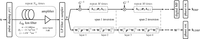
Fig. 1: Block diagram showing the end-to-end system model (LP: low-pass, MF: matched filter). The top processing branch corresponds to DBP via the SSFM and the bottom branch to the proposed learned DBP (LDBP), obtained by “unrolling” the SSFM. Prior to the parameter optimization via deep learning, LDBP has the same performance as DBP assuming the same number of steps/layers per span.

The main idea in this paper is to interpret the SSFM in (2) as a blueprint for a complex-valued deep NN and optimize the network parameters using machine learning tools. We refer to the resulting method as learned DBP (LDBP).

In the following, we consider a multi-span system where the optical link consists of $N_{\text{sp}}$ spans of length $L_{\text{sp}}$, as shown in Fig. 1. An optical amplifier is inserted after each span to compensate for the signal attenuation. In the SSFM, this is accounted for by including multiplicative factors $G^{-1}=e^{-\frac{\alpha}{2}L_{\text{sp}}}$ as shown in the top processing branch in Fig. 1. The estimated symbol vector $\hat{\mathbf{x}}_{\text{DBP}}\in\mathbb{C}^{m}$ is obtained by applying a digital MF followed by a phase-offset rotation.

4.1 Neural network parameters

The bottom branch in Fig. 1 shows an example for the NN in LDBP based on unrolling the SSFM with $M=2$ steps per span (StPS). Each network layer comprises two weight matrices $\smash{\mathbf{W}^{(i)}_{1},\mathbf{W}^{(i)}_{2}\in\mathbb{C}^{n\times n}}$ (no bias vectors are used). For the $i$-th layer, the nonlinearity $\smash{\bm{\rho}^{(i)}:\mathbb{C}^{n}\to\mathbb{C}^{n}}$ acts element-wise using $\rho^{(i)}(x)=xe^{-j\alpha_{i}|x|^{2}}$ in each dimension, where $\alpha_{i},x\in\mathbb{C}$. The function $\rho^{(i)}$ is differentiable and can thus be used with standard gradient-based optimization algorithms for deep learning. The MF is accounted for by inserting an additional linear layer with weight matrix $\mathbf{W}^{(\ell)}\in\mathbb{C}^{n\times m}$, where $\ell=MN_{\text{sp}}+1$ is the total number of network layers.

The network parameters are $\theta=\{\smash{\mathbf{W}^{(1)}_{1},\dots,\mathbf{W}^{(\ell-1)}_{1},\mathbf{W}^{(1)}_{2},\dots,\mathbf{W}^{(\ell-1)}_{2},\mathbf{W}^{(\ell)}},\alpha_{1},\dots,\alpha_{\ell-1}\}$. For the optimization, all weight matrices are restricted to an equivalent circular convolution with a symmetric filter of length $2K+1$. That is, the matrix rows are circularly shifted versions of $(h_{-K},\dots,h_{-1},h_{0},h_{1},\dots,h_{K},0,\dots,0)$, where $h_{i}\in\mathbb{C}$ and $h_{-i}=h_{i}$ for $i=1,2,\dots,K$. This reduces the number of free (complex-valued) parameters per weight matrix from $n^{2}$ to $K+1$, where $K\ll n$. This restriction also implies that LDBP is fully compatible with a potential time-domain filter implementation [13]. The weight matrices are initialized by using the appropriately zeroed versions of $\smash{\mathbf{A}_{\delta/2}}$, multiplied by $G^{-1}$ for $\smash{\mathbf{W}_{1}^{(i)}}$ in the first layer of each span. Furthermore, we initialize $\alpha_{i}=\gamma\delta$ and set $\smash{\mathbf{W}^{(\ell)}}$ to the MF. Thus, prior to the parameter optimization, LDBP has the same performance as DBP with the same number of StPS (assuming sufficiently large $K$).

4.2 Objective function and optimization procedure

NNs are trained by using many pairs of input and desired–output examples and adjusting the network parameters $\theta$ such that some predefined loss function between the network output and the desired output decreases. For LDBP, the network input is $\mathbf{y}\in\mathbb{C}^{n}$ and the desired output is the transmitted symbol vector $\mathbf{x}\in\mathcal{X}^{m}$. As a loss function, we use the mean squared error $\|\mathbf{x}-\hat{\mathbf{x}}_{\text{LDBP}}\|$, where $\|\mathbf{x}\|\triangleq\sum_{i=1}^{m}|x_{i}|^{2}$ and $\hat{\mathbf{x}}_{\text{LDBP}}\in\mathbb{C}^{m}$ denotes the NN output of LDBP. Assuming that $\|\mathbf{x}\|$ is constant for all $\mathbf{x}$, this is equivalent to maximizing the Q-factor $\|\mathbf{x}\|/\|\mathbf{x}-\hat{\mathbf{x}}_{\text{LDBP}}\|$. We used TensorFlow to implement the NN and optimize the network parameters. For the optimization, we use the built-in Adam optimizer, which performs stochastic gradient descent with 30 input–output pairs $(\mathbf{y},\mathbf{x})$ (i.e., mini-batches) per optimization step.

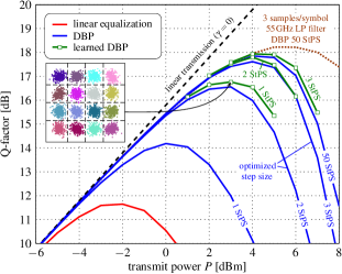
Fig. 2: Results

Our system setup is such that the training data is generated on-the-fly utilizing all CPU cores, whereas the gradient-descent optimization is performed in parallel on the same machine using an NVIDIA Tesla K40c GPU.

5 Numerical results

We assume $16$-QAM transmission at $20\,$Gbaud using root-raised cosine pulses (roll-off factor 0.1). For the optical link, we set $N_{\text{sp}}=32$ and $L_{\text{sp}}=100\,$km with fiber parameters shown in Fig. 1. Brick-wall LP filtering with $35\,$GHz bandwidth is applied before sampling at $f_{\text{samp}}=40\,$GHz, i.e., 2 samples/symbol are used for the receiver processing. Forward propagation is simulated using 6 samples/symbol and $50$ StPS in the SSFM (increasing either value did not affect the results). We consider LDBP with 1, 2, and 3 StPS, where the filter memory $K$ is set to $12$, $8$, and $6$, respectively. The resulting Q-factor is shown in Fig. 2. During the optimization, the transmit power for a particular input–output pair is chosen randomly from the set of powers that is shown by the markers in Fig. 2, e.g., $P\in\{1,2,3,4,5\}$ dBm for LDBP with 1 StPS. As a comparison, we show the performance of DBP via the SSFM with 1, 2, 3, and 50 StPS. For 2 and 3 StPS, we used an optimized (non-uniform) step size per span. At the optimal transmit power, LDBP with 1 StPS provides a Q-factor of $16.8\,$dB compared to $16.6\,$dB for DBP with 2 StPS. Taking the number of StPS as a rough measure of complexity, LDBP thus gives a 50% complexity reduction over DBP for comparable performance. Moreover, due to the relatively short filter memory $K$, a time-domain implementation may be preferred over the use of Fourier transforms to implement the linear convolutions [13]. As seen in Fig. 2, using more StPS gives diminishing returns in terms of the achievable Q-factor for both LDBP and DBP. However, it is noteworthy that LDBP with 3 StPS slightly outperforms DBP with 50 StPS in the nonlinear regime (although the optimal Q-factor is essentially the same). This is likely due to the fact that a significant part of the broadened spectrum of the received waveform is filtered out before processing. While LDBP compensates somewhat for this effect, the missing spectrum is not backpropagated correctly when using DBP. In that case, a larger receiver bandwidth is necessary as shown in Fig. 2 by the dotted line.

6 Conclusion and future work

We have proposed an approach for NLI mitigation using deep NNs, where the network design is based on unrolling the SSFM. Compared to standard “black-box” deep NNs, this approach leads to clear hyperparameter choices (e.g., number of network layers, type of nonlinearity, etc.) and also provides a good initialization for the gradient-based optimization. The resulting learned DBP significantly reduces the complexity compared to conventional DBP implementations.

One of the most appealing features of NNs is that they can adapt to real-world imperfections that are not included in analytical models such as (1). For future work, it would therefore be interesting to perform the parameter optimization based on experimental data. It could also be viable to explore NN designs for LDBP that include modified nonlinear functions, e.g., with additional filtering steps [3], in order to further improve the performance–complexity trade-off.

References

- [1]
- [2] E. Ip and J. M. Kahn, “Compensation of dispersion and nonlinear impairments using digital backpropagation,” J. Lightw. Technol. 26, 3416–3425 (2008).
- [3] L. B. Du and A. J. Lowery, “Improved single channel backpropagation for intra-channel fiber nonlinearity compensation in long-haul optical communication systems.” Opt. Express 18, 17,075–17,088 (2010).
- [4] Z. Tao et al., “Multiplier-free intrachannel nonlinearity compensating algorithm operating at symbol rate,” J. Lightw. Technol. 29, 2570–2576 (2011).
- [5] L. Li et al., “Implementation efficient nonlinear equalizer based on correlated digital backpropagation,” in “Proc. OFC,” (Los Angeles, CA, 2011).
- [6] T. Shen and A. Lau, “Fiber nonlinearity compensation using extreme learning machine for DSP-based coherent communication systems,” in “Proc. OECC,” (Kaohsiung, Taiwan, 2011).
- [7] A. M. Jarajreh et al., “Artificial neural network nonlinear equalizer for coherent optical OFDM,” IEEE Photon. Technol. Lett. 27, 387–390 (2015).
- [8] E. Giacoumidis et al., “Fiber nonlinearity-induced penalty reduction in CO-OFDM by ANN-based nonlinear equalization,” Opt. Lett. 40, 5113–5116 (2015).
- [9] Y. LeCun et al., “Deep learning,” Nature 521, 436–444 (2015).
- [10] K. Gregor and Y. Lecun, “Learning fast approximations of sparse coding,” in “Proc. ICML,” (Haifa, Israel, 2010).
- [11] E. Nachmani et al., “Learning to decode linear codes using deep learning,” in “Proc. Allerton Conf.,” (Illinois, USA, 2016).
- [12] H. W. Lin et al., “Why does deep and cheap learning work so well?” J. Stat. Phys. 168, 1223–1247 (2017).
- [13] C. Fougstedt et al., “Time-domain digital back propagation: Algorithm and finite-precision implementation aspects,” in “Proc. OFC,” (Los Angeles, USA, 2017).