Minimax Estimation of Bandable Precision Matrices

Abstract

The inverse covariance matrix provides considerable insight for understanding statistical models in the multivariate setting. In particular, when the distribution over variables is assumed to be multivariate normal, the sparsity pattern in the inverse covariance matrix, commonly referred to as the precision matrix, corresponds to the adjacency matrix representation of the Gauss-Markov graph, which encodes conditional independence statements between variables. Minimax results under the spectral norm have previously been established for covariance matrices, both sparse and banded, and for sparse precision matrices. We establish minimax estimation bounds for estimating banded precision matrices under the spectral norm. Our results greatly improve upon the existing bounds; in particular, we find that the minimax rate for estimating banded precision matrices matches that of estimating banded covariance matrices. The key insight in our analysis is that we are able to obtain barely-noisy estimates of $k\times k$ subblocks of the precision matrix by inverting slightly wider blocks of the empirical covariance matrix along the diagonal. Our theoretical results are complemented by experiments demonstrating the sharpness of our bounds.

1 Introduction

Imposing structure is crucial to performing statistical estimation in the high-dimensional regime where the number of observations can be much smaller than the number of parameters. In estimating graphical models, a long line of work has focused on understanding how to impose sparsity on the underlying graph structure.

Sparse edge recovery is generally not easy for an arbitrary distribution. However, for Gaussian graphical models, it is well-known that the graphical structure is encoded in the inverse of the covariance matrix $\Sigma^{-1}=\Omega$, commonly referred to as the precision matrix [12, 14, 3]. Therefore, accurate recovery of the precision matrix is paramount to understanding the structure of the graphical model. As a consequence, a great deal of work has focused on sparse recovery of precision matrices under the multivariate normal assumption [8, 4, 5, 17, 16]. Beyond revealing the graph structure, the precision matrix also turns out to be highly useful in a variety of applications, including portfolio optimization, speech recognition, and genomics [12, 23, 18].

Although there has been a rich literature exploring the sparse precision matrix setting for Gaussian graphical models, less work has emphasized understanding the estimation of precision matrices under additional structural assumptions, with some exceptions for block structured sparsity [11] or bandability [1]. One would hope that extra structure should allow us to obtain more statistically efficient solutions. In this work, we focus on the case of bandable precision matrices, which capture a sense of locality between variables. Bandable matrices arise in a number of time-series contexts and have applications in climatology, spectroscopy, fMRI analysis, and astronomy [9, 20, 15]. For example, in the time-series setting, we may assume that edges between variables $X_{i},X_{j}$ are more likely when $i$ is temporally close to $j$, as is the case in an auto-regressive process. The precision and covariance matrices corresponding to distributions with this property are referred to as bandable, or tapering. We will discuss the details of this model in the sequel.

Past work:

Previous work has explored the estimation of both bandable covariance and precision matrices [6, 15]. Closely related work includes the estimation of sparse precision and covariance matrices [3, 17, 4]. Asymptotically-normal entrywise precision estimates as well as minimax rates for operator norm recovery of sparse precision matrices have also been established [16]. A line of work developed concurrently to our own establishes a matching minimax lower bound [13].

When considering an estimation technique, a powerful criterion for evaluating whether the technique performs optimally in terms of convergence rate is minimaxity. Past work has established minimax rates of convergence for sparse covariance matrices, bandable covariance matrices, and sparse precision matrices [7, 6, 4, 17].

The technique for estimating bandable covariance matrices proposed in [6] is shown to achieve the optimal rate of convergence. However, no such theoretical guarantees have been shown for the bandable precision estimator proposed in recent work for estimating sparse and smooth precision matrices that arise from cosmological data [15].

Of note is the fact that the minimax rate of convergence for estimating sparse covariance matrices matches the minimax rate of convergence of estimating sparse precision matrices. In this paper, we introduce an adaptive estimator and show that it achieves the optimal rate of convergence when estimating bandable precision matrices from the banded parameter space (3). We find, satisfyingly, that analogous to the sparse case, in which the minimax rate of convergence enjoys the same rate for both precision and covariance matrices, the minimax rate of convergence for estimating bandable precision matrices matches the minimax rate of convergence for estimating bandable covariance matrices that has been established in the literature [6].

Our contributions:

Our goal is to estimate a banded precision matrix based on $n$ i.i.d. observations. We consider a parameter space of precision matrices $\Omega$ with a power law decay structure nearly identical to the bandable covariance matrices considered for covariance matrix estimation [6]. We present a simple-to-implement algorithm for estimating the precision matrix. Furthermore, we show that the algorithm is minimax optimal with respect to the spectral norm. The upper and lower bounds given in Section 3 together imply the following optimal rate of convergence for estimating bandable precision matrices under the spectral norm. Informally, our results show the following bound for recovering a banded precision matrix with bandwidth $k$.

Theorem 1.1 (Informal).

The minimax risk for estimating the precision matrix $\Omega$ over the class $\mathcal{P}_{\alpha}$ given in (3) satisfies:

$$\inf_{\hat{\Omega}}\sup_{\mathcal{P}_{\alpha}}\operatorname{\mathbf{E}}\left\lVert\hat{\Omega}-\Omega\right\rVert^{2}\approx\frac{k+\log p}{n}$$ (1)

where this bound is achieved by the tapering estimator $\hat{\Omega}_{k}$ as defined in Equation (7).

An important point to note, which is shown more precisely in the sequel, is that the rate of convergence as compared to sparse precision matrix recovery is improved by a factor of $\min(k\log(p),k^{2})$.

We establish a minimax upper bound by detailing an algorithm for obtaining an estimator given observations $\mathbf{x}_{1},\dotsc,\mathbf{x}_{n}$ and a pre-specified bandwidth $k$, and studying the resultant estimator’s risk properties under the spectral norm. We show that an estimator using our algorithm with the optimal choice of bandwidth attains the minimax rate of convergence with high probability.

To establish the optimality of our estimation routine, we derive a minimax lower bound to show that the rate of convergence cannot be improved beyond that of our estimator. The lower bound is established by constructing subparameter spaces of (3) and applying testing arguments through Le Cam’s method and Assouad’s Lemma [22, 6].

To supplement our analysis, we conduct numerical experiments to explore the performance of our estimator in the finite sample setting. The numerical experiments confirm that even in the finite sample case, our proposed estimator exhibits the minimax rate of convergence.

The remainder of the paper is organized as follows. In Section 2, we detail the exact model setting and introduce a blockwise inversion technique for precision matrix estimation. In Section 3, theorems establishing the minimaxity of our estimator under the spectral norm are presented. An upper bound on the estimator’s risk is given in high probability with the help of a result from set packing. The minimax lower bound is derived by way of a testing argument. Both bounds are accompanied by their proofs. Finally, in Section 4, our estimator is subjected to numerical experiments. Owing to space constraints, proofs for auxiliary lemmas may be found in Appendix A.

Notation:

We will now collect notation that will be used throughout the remaining sections. Vectors will be denoted as lower-case $\mathbf{x}$ while matrices are upper-case $A$. The spectral or operator norm of a matrix is defined to be $\left\lVert A\right\rVert=\sup_{\mathbf{x}\neq 0,\mathbf{y}\neq 0}\langle A\mathbf{x},\mathbf{y}\rangle$ while the matrix $\ell_{1}$ norm of a symmetric matrix $A\in\mathbf{R}^{m\times m}$ is defined to be $\left\lVert A\right\rVert_{1}=\max_{j}\sum_{i=1}^{m}|A_{ij}|$.

2 Background and problem set-up

In this section we present details of our model and the estimation procedure. If one considers observations of the form $\mathbf{x}_{1},\dotsc,\mathbf{x}_{n}\in\mathbf{R}^{p}$ drawn from a distribution with precision matrix $\Omega_{p\times p}$ and zero mean, the goal then is to estimate the unknown matrix $\Omega_{p\times p}$ based on the observations $\{\mathbf{x}_{i}\}_{i=1}^{n}$. Given a random sample of $p$-variate observations $\mathbf{x}_{1},\dotsc,\mathbf{x}_{n}$ drawn from a multivariate distribution with population covariance $\Sigma=\Sigma_{p\times p}$, our procedure is based on a tapering estimator derived from blockwise estimates for estimating the precision matrix $\Omega_{p\times p}=\Sigma^{-1}$.

The maximum likelihood estimator of $\Sigma$ is

$$\hat{\Sigma}=(\hat{\sigma}_{ij})_{1\leq i,j\leq p}=\frac{1}{n}\sum_{l=1}^{n}(\mathbf{x}_{l}-\bar{\mathbf{x}})(\mathbf{x}_{l}-\bar{\mathbf{x}})^{\top}$$ (2)

where $\bar{\mathbf{x}}$ is the empirical mean of the vectors $\mathbf{x}_{i}$. We will construct estimators of the precision matrix $\Omega=\Sigma^{-1}$ by inverting blocks of $\hat{\Sigma}$ along the diagonal, and averaging over the resultant subblocks.

Throughout this paper we adhere to the convention that $\omega_{ij}$ refers to the $ij^{\text{th}}$ element in a matrix $\Omega$. Consider the parameter space $\mathcal{F}_{\alpha}$, with associated probability measure $\mathcal{P}_{\alpha}$, given by:

$$\mathcal{F}_{\alpha}=\mathcal{F}_{\alpha}(M_{0},M)=\Bigg{\{}\Omega:\max_{j}\sum_{i}\left\{|\omega_{ij}|:|i-j|\geq k\right\}\leq Mk^{-\alpha}\text{ for all }k,\lambda_{i}(\Omega)\in[M_{0}^{-1},M_{0}]\Bigg{\}}$$ (3)

where $\lambda_{i}(\Omega)$ denotes the $i$th eigenvalue of $\Omega$, with $\lambda_{i}\geq\lambda_{j}$ for all $i\leq j$. We also constrain $\alpha>0,M>0,M_{0}>0$. Observe that this parameter space is nearly identical to that given in Equation (3) of [6]. We take on an additional assumption on the minimum eigenvalue of $\Omega\in\mathcal{F}_{\alpha}$, which is used in the technical arguments where the risk of estimating $\Omega$ under the spectral norm is bounded in terms of the error of estimating $\Sigma=\Omega^{-1}$.

Observe that the parameter space intuitively dictates that the magnitude of the entries of $\Omega$ decays in power law as we move away from the diagonal. As with the parameter space for bandable covariance matrices given in [6], we may understand $\alpha$ in (3) as a rate of decay for the precision entries $\omega_{ij}$ as they move away from the diagonal; it can also be understood in terms of the smoothness parameter in nonparametric estimation [19]. As will be discussed in Section 3, the optimal choice of $k$ depends on both $n$ and the decay rate $\alpha$.

2.1 Estimation procedure

We now detail the algorithm for obtaining minimax estimates for bandable $\Omega$, which is also given as pseudo-code in Algorithm 1.

The algorithm is inspired by the tapering procedure introduced by Cai, Zhang, and Zhou [6] in the case of covariance matrices, with modifications in order to estimate the precision matrix. Estimating the precision matrix introduces new difficulties as we do not have direct access to the estimates of elements of the precision matrix. For a given integer $k,1\leq k\leq p$, we construct a tapering estimator as follows. First, we calculate the maximum likelihood estimator for the covariance, as given in Equation (2). Then, for all integers $1-m\leq l\leq p$ and $m\geq 1$, we define the matrices with square blocks of size at most $3m$ along the diagonal:

$$\hat{\Sigma}_{l-m}^{(3m)}=(\hat{\sigma}_{ij}\mathbf{1}\{l-m\leq i<l+2m,l-m\leq j<l+2m\})_{p\times p}$$ (4)

For each $\hat{\Sigma}_{l-m}^{(3m)}$, we replace the nonzero block with its inverse to obtain $\breve{\Omega}_{l-m}^{(3m)}$. For a given $l$, we refer to the individual entries of this intermediate matrix as follows:

$$\breve{\Omega}_{l-m}^{(3m)}=(\breve{\omega}^{l}_{ij}\mathbf{1}\{l-m\leq i<l+2m,l-m\leq j<l+2m\})_{p\times p}$$ (5)

For each $l$, we then keep only the central $m\times m$ subblock of $\breve{\Omega}_{l-m}^{(3m)}$ to obtain the blockwise estimate $\hat{\Omega}_{l}^{(m)}$:

$$\hat{\Omega}_{l}^{(m)}=(\breve{\omega}^{l}_{ij}\mathbf{1}\{l\leq i<l+m,l\leq j<l+m\})_{p\times p}$$ (6)

Note that this notation allows for $l<0$ and $l+m>p$; in each case, this out-of-bounds indexing allows us to cleanly handle corner cases where the subblocks are smaller than $m\times m$.

For a given bandwidth $k$ (assume $k$ is divisible by 2), we calculate these blockwise estimates for both $m=k$ and $m=\frac{k}{2}$. Finally, we construct our estimator by averaging over the block matrices:

$$\hat{\Omega}_{k}=\frac{2}{k}\cdot\left(\sum_{l=1-k}^{p}\hat{\Omega}_{l}^{(k)}-\sum_{l=1-\nicefrac{{k}}{{2}}}^{p}\hat{\Omega}_{l}^{(\nicefrac{{k}}{{2}})}\right)$$ (7)

We note that within $\frac{k}{2}$ entries of the diagonal, each entry is effectively the sum of $\frac{k}{2}$ estimates, and as we move from $\frac{k}{2}$ to $k$ from the diagonal, each entry is progressively the sum of one fewer entry.

Therefore, within $\frac{k}{2}$ of the diagonal, the entries are not tapered; and from $\frac{k}{2}$ to $k$ of the diagonal, the entries are linearly tapered to zero. The analysis of this estimator makes careful use of this tapering schedule and the fact that our estimator is constructed through the average of block matrices of size at most $k\times k$.

function FitBlockwise($\hat{\Sigma}$, k)

     $\hat{\Omega}\leftarrow\mathbf{0}_{p\times p}$

     for $l\in[1-k,p)$ do

         $\hat{\Omega}\leftarrow\hat{\Omega}+\textsc{BlockInverse}(\hat{\Sigma},k,l)$

     end for

     for $l\in[1-\lfloor\nicefrac{{k}}{{2}}\rfloor,p)$ do

         $\hat{\Omega}\leftarrow\hat{\Omega}-\textsc{BlockInverse}(\hat{\Sigma},\lfloor\nicefrac{{k}}{{2}}\rfloor,l)$

     end for

     return $\hat{\Omega}$

end function

function BlockInverse($\hat{\Sigma}$, m, l)

     $\triangleright$ Obtain $3m\times 3m$ block inverse.

     $s\leftarrow\max\{l-m,0\}$

     $f\leftarrow\min\{p,l+2m\}$

     $M\leftarrow\left(\hat{\Sigma}\texttt{[s:f, s:f]}\right)^{-1}$

     $\triangleright$ Preserve central $m\times m$ block of inverse.

     $s\leftarrow m+\min\{l-m,0\}$

     $N\leftarrow M\texttt{[s:s+m, s:s+m]}$

     $\triangleright$ Restore block inverse to appropriate indices.

     $s\leftarrow\max\{l,0\}$

     $f\leftarrow\min\{l+m,p\}$

     $P\texttt{[s:f, s:f]}=N$

     return $P$

end function

Algorithm 1 Blockwise Inversion Technique

2.2 Implementation details

The naive algorithm performs $O(p+k)$ inversions of square matrices with size at most $3k$. This method can be sped up considerably through an application of the Woodbury matrix identity and the Schur complement relation [21, 2]. Doing so reduces the computational complexity of the algorithm from $O(pk^{3})$ to $O(pk^{2})$. We discuss the details of modified algorithm and its computational complexity below.

Suppose we have $\breve{\Omega}_{l-m}^{(3m)}$ and are interested in obtaining $\breve{\Omega}_{l-m+1}^{(3m)}$. We observe that the nonzero block of $\breve{\Omega}_{l-m+1}^{(3m)}$ corresponds to the inverse of the nonzero block of $\hat{\Sigma}_{l-m+1}^{(3m)}$, which only differs by one row and one column from $\hat{\Sigma}_{l-m}^{(3m)}$, the matrix for which the inverse of the nonzero block corresponds to $\breve{\Omega}_{l-m}^{(3m)}$, which we have already computed. We may understand the movement from $\hat{\Sigma}_{l-m}^{(3m)},\breve{\Omega}_{l-m}^{(3m)}$ to $\hat{\Sigma}_{l-m+1}^{(3m)}$ (to which we already have direct access) and $\breve{\Omega}_{l-m+1}^{(3m)}$ as two rank-1 updates. Let us view the nonzero blocks of $\hat{\Sigma}_{l-m}^{(3m)},\breve{\Omega}_{l-m}^{(3m)}$ as the block matrices:

$$\mathrm{NonZero}(\hat{\Sigma}_{l-m}^{3m}) =\begin{bmatrix}A\in\mathbf{R}^{1\times 1}&B\in\mathbf{R}^{1\times(3m-1)}\\ B^{\top}\in\mathbf{R}^{(3m-1)\times 1}&C\in\mathbf{R}^{(3m-1)\times(3m-1)}\end{bmatrix}$$

$$\mathrm{NonZero}(\breve{\Omega}_{l-m}^{(3m)}) =\begin{bmatrix}\tilde{A}\in\mathbf{R}^{1\times 1}&\tilde{B}\in\mathbf{R}^{1\times(3m-1)}\\ \tilde{B}^{\top}\in\mathbf{R}^{(3m-1)\times 1}&\tilde{C}\in\mathbf{R}^{(3m-1)\times(3m-1)}\end{bmatrix}$$

The Schur complement relation tells us that given $\hat{\Sigma}_{l-m}^{3m},\breve{\Omega}_{l-m}^{(3m)}$, we may trivially compute $C^{-1}$ as follows:

$$C^{-1}=\left(\tilde{C}^{-1}+B^{\top}A^{-1}B\right)^{-1}=\tilde{C}-\frac{\tilde{C}B^{\top}B\tilde{C}}{A+B\tilde{C}B^{\top}}$$ (8)

by the Woodbury matrix identity, which gives an efficient algorithm for computing the inverse of a matrix subject to a low-rank (in this case, rank-1) perturbation. This allows us to move from the inverse of a matrix in $\mathbf{R}^{3m\times 3m}$ to the inverse of a matrix in $\mathbf{R}^{(3m-1)\times(3m-1)}$ where a row and column have been removed. A nearly identical argument allows us to move from the $\mathbf{R}^{(3m-1)\times(3m-1)}$ matrix to an $\mathbf{R}^{3m\times 3m}$ matrix where a row and column have been appended, which gives us the desired block of $\breve{\Omega}_{l-m+1}^{(3m)}$.

With this modification to the algorithm, we need only compute the inverse of a square matrix of width $2m$ at the beginning of the routine; thereafter, every subsequent block inverse may be computed through simple rank one matrix updates.

2.3 Complexity details

We now detail the factor of $k$ improvement in computational complexity provided through the application of the Woodbury matrix identity and the Schur complement relation introduced in Section 2.2. Recall that the naive implementation of Algorithm 1 involves $O(p+k)$ inversions of square matrices of size at most $3k$, each of which cost $O(k^{3})$. Therefore, the overall complexity of the naive algorithm is $O(pk^{3})$, as $k<p$.

Now, consider the Woodbury-Schur-improved algorithm. The initial single inversion of a $2k\times 2k$ matrix costs $O(k^{3})$. Thereafter, we perform $O(p+k)$ updates of the form given in Equation (8). These updates simply require vector matrix operations. Therefore, the update complexity on each iteration is $O(k^{2})$. It follows that the overall complexity of the amended algorithm is $O(pk^{2})$.

3 Rate optimality under the spectral norm

Here we present the results that establish the rate optimality of the above estimator under the spectral norm. For symmetric matrices $A$, the spectral norm, which corresponds to the largest singular value of $A$, coincides with the $\ell_{2}$-operator norm. We establish optimality by first deriving an upper bound in high probability using the blockwise inversion estimator defined in Section 2.1. We then give a matching lower bound in expectation by carefully constructing two sets of multivariate normal distributions and then applying Assouad’s Lemma and Le Cam’s method.

3.1 Upper bound under the spectral norm

In this section we derive a risk upper bound for the tapering estimator defined in (7) under the operator norm. We assume the distribution of the $\mathbf{x}_{i}$’s is subgaussian; that is, there exists $\rho>0$ such that:

$$\mathbf{P}\left\{|\mathbf{v}^{\top}(\mathbf{x}_{i}-\operatorname{\mathbf{E}}\mathbf{x}_{i})|>t\right\}\leq e^{-\frac{t^{2}\rho}{2}}$$ (9)

for all $t>0$ and $\left\lVert\mathbf{v}\right\rVert_{2}=1$. Let $\mathcal{P}_{\alpha}=\mathcal{P}_{\alpha}(M_{0},M,\rho)$ denote the set of distributions of $\mathbf{x}_{i}$ that satisfy (3) and (9).

Theorem 3.1.

The tapering estimator $\hat{\Omega}_{k}$, defined in (7), of the precision matrix $\Omega_{p\times p}$ with $p>n^{\frac{1}{2\alpha+1}}$ satisfies:

$$\sup_{\mathcal{P}_{\alpha}}\mathbf{P}\left\{\left\lVert\hat{\Omega}_{k}-\Omega\right\rVert^{2}\geq C\frac{k+\log p}{n}+Ck^{-2\alpha}\right\}=O\left(p^{-15}\right)$$ (10)

with $k=o(n)$, $\log p=o(n)$, and a universal constant $C>0$.

In particular, the estimator $\hat{\Omega}=\hat{\Omega}_{k}$ with $k=n^{\frac{1}{2\alpha+1}}$ satisfies:

$$\sup_{\mathcal{P}_{\alpha}}\mathbf{P}\left\{\left\lVert\hat{\Omega}_{k}-\Omega\right\rVert^{2}\geq Cn^{-\frac{2\alpha}{2\alpha+1}}+C\frac{\log p}{n}\right\}=O\left(p^{-15}\right)$$ (11)

Given the result in Equation (10), it is easy to show that setting $k=n^{\frac{1}{2\alpha+1}}$ yields the optimal rate by balancing the size of the inside-taper and outside-taper terms, which gives Equation (11).

The proof of this theorem, which is given next, relies on the fact that when we invert a $3k\times 3k$ block, the difference between the central $k\times k$ block and the corresponding $k\times k$ block which would have been obtained by inverting the full matrix has a negligible contribution to the risk. As a result, we are able to take concentration bounds on the operator norm of subgaussian matrices, customarily used for bounding the norm of the difference of covariance matrices, and apply them instead to differences of precision matrices to obtain our result.

The key insight is that we can relate the spectral norm of a $k\times k$ subblock produced by our estimator to the spectral norm of the corresponding $k\times k$ subblock of the covariance matrix, which allows us to apply concentration bounds from classical random matrix theory. Moreover, it turns out that if we apply the tapering schedule induced by the construction of our estimator to the population parameter $\Omega\in\mathcal{F}_{\alpha}$, we may express the tapered population $\Omega$ as a sum of block matrices in exactly the same way that our estimator is expressed as a sum of block matrices.

In particular, the tapering schedule is presented next. Suppose a population precision matrix $\Omega\in\mathcal{F}_{\alpha}$. Then, we denote the tapered version of $\Omega$ by $\Omega_{A}$, and construct:

$$\Omega_{A} =\left(\omega_{ij}\cdot v_{ij}\right)_{p\times p}$$

$$\Omega_{B} =\left(\omega_{ij}\cdot(1-v_{ij}\right))_{p\times p}$$

where the tapering coefficients are given by:

$$v_{ij}=\begin{cases}1&\text{ for }|i-j|<\frac{k}{2}\\ \frac{|i-j|}{\nicefrac{{k}}{{2}}}&\text{ for }\frac{k}{2}\leq|i-j|<k\\ 0&\text{ for }|i-j|\geq k\\ \end{cases}$$

We then handle the risk of estimating the inside-taper $\Omega_{A}$ and the risk of estimating the outside-taper $\Omega_{B}$ separately.

Because our estimator and the population parameter are both averages over $k\times k$ block matrices along the diagonal, we may then take a union bound over the high probability bounds on the spectral norm deviation for the $k\times k$ subblocks to obtain a high probability bound on the risk of our estimator.

3.1.1 Proof of Theorem 3.1

The main step in proving the upper bound on the estimation rate is bounding the error for a tapered version of the truth and its complement separately. Let us denote a tapering coefficient:

$$v_{ij}=\begin{cases}1&\text{ for }|i-j|<\frac{k}{2}\\ \frac{|i-j|}{\nicefrac{{k}}{{2}}}&\text{ for }\frac{k}{2}\leq|i-j|<k\\ 0&\text{ for }|i-j|\geq k\\ \end{cases}$$ (12)

Let us denote:

$$\Omega_{A} =\left(\omega_{ij}\cdot v_{ij}\right)_{p\times p}$$

$$\Omega_{B} =\left(\omega_{ij}\cdot(1-v_{ij}\right))_{p\times p}$$

We similarly decompose:

$$\hat{\Omega}_{A} =\left(\hat{\omega}_{ij}\cdot\mathbf{1}\{|i-j|<k\}\right)_{p\times p}$$

$$\hat{\Omega}_{B} =\left(\hat{\omega}_{ij}\cdot\mathbf{1}\{|i-j|\geq k\}\right)_{p\times p}$$

We will first show that the error against the tapered truth satisfies:

$$\mathbf{P}\left\{\left\lVert\hat{\Omega}_{A}-\Omega_{A}\right\rVert^{2}\geq C\left(\frac{k+\log p}{n}\right)+Ck^{-4a}\right\}=O\left(p^{-15}\right)$$ (13)

and that the error outside the taper satisfies the deterministic bound:

$$\left\lVert\hat{\Omega}_{B}-\Omega_{B}\right\rVert^{2}\leq Ck^{-2\alpha}$$ (14)

It then follows that:

$$\mathbf{P} \left\{\left\lVert\hat{\Omega}-\Omega\right\rVert^{2}\geq C\frac{k+\log p}{n}+Ck^{-2\alpha}\right\}$$

$$\leq\mathbf{P}\left\{2\left\lVert\hat{\Omega}_{A}-\Omega_{A}\right\rVert^{2}+2\left\lVert\hat{\Omega}_{B}-\Omega_{B}\right\rVert^{2}\geq C\frac{k+\log p}{n}+Ck^{-4\alpha}+Ck^{-2\alpha}\right\}$$

$$\leq\mathbf{P}\left\{\left\lVert\hat{\Omega}_{A}-\Omega_{A}\right\rVert^{2}\geq C\frac{k+\log p}{n}+Ck^{-4\alpha}\right\}+\mathbf{P}\left\{\left\lVert\hat{\Omega}_{B}-\Omega_{B}\right\rVert^{2}\geq Ck^{-2\alpha}\right\}$$

$$=O\left(p^{-15}\right)$$

This proves (10), from which follows (11). Therefore, the estimator $\hat{\Omega}$ with $k=n^{\frac{1}{2\alpha+1}}$ satisfies:

$$\mathbf{P}\left\{\left\lVert\hat{\Omega}-\Omega\right\rVert^{2}\leq 2C\left(n^{-\frac{2\alpha}{2\alpha+1}}+\frac{\log p}{n}\right)\right\} =O\left(p^{-15}\right)$$

This proves Theorem 3.1.

We first establish (14), which is relatively simple. Observe that by definition, $\hat{\Omega}_{B}$ is the zero matrix, as $\hat{\Omega}$ already sets all entries outside the band to zero. Therefore:

$$\left\lVert\hat{\Omega}_{B}-\Omega_{B}\right\rVert^{2} =\left\lVert\Omega_{B}\right\rVert^{2}$$

$$\leq\left\lVert\Omega_{B}\right\rVert_{1}^{2}$$

$$=\left[\max_{j}\sum_{i}|\omega_{ij}\cdot(1-v_{ij})|\right]^{2}$$

$$\leq\left[\max_{j}\sum_{|i-j|>\frac{k}{2}}|\omega_{ij}|\right]^{2}$$

$$\leq\left[M2^{\alpha}k^{-\alpha}\right]^{2}$$

$$=Ck^{-2\alpha}$$

We now show (13). Let $\Omega_{l}^{(m)}=(\omega_{ij}\mathbf{1}\{l\leq i<l+m,l\leq j<l+m\})_{p\times p}$.

Lemma 1.

We may express the tapered population parameter as:

$$\Omega_{A}=\frac{2}{k}\cdot\left(\sum_{l=1-k}^{p}\Omega_{l}^{(k)}-\sum_{l=1-\nicefrac{{k}}{{2}}}^{p}\Omega_{l}^{(\nicefrac{{k}}{{2}})}\right)$$ (15)

Then define:

$$N^{(m)}=\max_{1-m\leq l\leq p}\left\lVert\hat{\Omega}_{l}^{(m)}-\Omega_{l}^{(m)}\right\rVert$$ (16)

Lemma 2.

Let $\hat{\Omega}=\hat{\Omega}_{m}$ be defined as in (7). Then

$$\left\lVert\hat{\Omega}-\Omega_{A}\right\rVert\leq C\cdot N^{(m)}$$

We then show that our estimation technique approximates each block of the true precision matrix up to a lower order correction.

Lemma 3.

The $m\times m$ block of $\Omega$ starting at the $l$th diagonal entry may be expressed as an approximation $\tilde{\Omega}_{l}^{(m)}$ from inverting blocks of the covariance matrix $\Sigma$ plus a correction term $W_{l}^{(m)}$.

$$\Omega_{l}^{(m)}=\tilde{\Omega}_{l}^{(m)}+W_{l}^{(m)}$$ (17)

In particular, $W_{l}^{(m)}$ takes the form:

$$W_{l}^{(m)}=\Omega_{B_{2}}\Omega_{C}^{-1}\Omega_{B_{2}}^{\top}$$

with:

$$\Omega_{B_{2}} =\begin{bmatrix}\Omega_{\alpha}&\Omega_{\beta}\end{bmatrix}$$

$$\Omega_{C} =\begin{bmatrix}\Omega_{\gamma}&\Omega_{\delta}^{\top}\\ \Omega_{\delta}&\Omega_{\epsilon}\end{bmatrix}$$

where we define the block matrices:

$$\Omega_{\alpha} =\Omega_{l\leq i<l+m,l+2m\leq j\leq p}$$

$$\Omega_{\beta} =\Omega_{l\leq i<l+m,1\leq j<l-m}$$

$$\Omega_{\gamma} =\Omega_{l+2m\leq i,j\leq p}$$

$$\Omega_{\delta} =\Omega_{l-m\leq i<l+2m,1\leq j<l-m}$$

$$\Omega_{\epsilon} =\Omega_{1\leq i,j<l-m}$$

and $\tilde{\Omega}_{l}^{(m)}$ is given by the central $m\times m$ block of $\Sigma_{l-m}^{(3m)^{-1}}$.

Lemma 4.

The correction factor $W$ in Lemma 3 is bounded in spectral norm:

$$\left\lVert W_{l}^{(m)}\right\rVert\leq Cm^{-2\alpha}$$ (18)

We may then control the operator norm of each $m\times m$ random matrix with $m=k$ as follows. First, we bound $N^{(m)}$ from above by two terms:

$$N^{(m)} =\max_{1-m\leq l\leq p}\left\lVert\hat{\Omega}_{l}^{(m)}-\Omega_{l}^{(m)}\right\rVert$$

$$\leq\underbrace{\max_{1-m\leq l\leq p}\left\lVert\hat{\Omega}_{l}^{(m)}-\tilde{\Omega}_{l}^{(m)}\right\rVert}_{N_{1}^{(m)}}+\underbrace{\max_{1-m\leq l\leq p}\left\lVert\tilde{\Omega}_{l}^{(m)}-\Omega_{l}^{(m)}\right\rVert}_{N_{2}^{(m)}}$$

Note that $N_{2}^{(m)}=\max_{l}\left\lVert W_{l}^{(m)}\right\rVert$. Therefore, we already have a deterministic bound on $N_{2}^{(m)}$ from Lemma 4.

Using standard results from random matrix theory we may bound $N_{1}^{(m)}$ with high probability in the following lemma. We defer the proof to the Appendix.

Lemma 5.

There exists a constant $\rho_{1}>0$ such that:

$$\mathbf{P}\left\{N_{1}^{(m)}>x\right\}\leq 2p\cdot 25^{3m}\exp\left\{-nx^{2}\rho_{1}\right\}$$ (19)

for all $0<x<\rho_{1}$ and $1-m\leq l\leq p$.

We now prove the upper bound in high probability on the within-band error in Equation (13). First, by setting $x=4\sqrt{\frac{\log p+m}{n\rho_{1}}}$, and recalling Lemma 5, we have:

$$\mathbf{P}\left\{\left(N_{1}^{(m)}\right)^{2}\geq 16\frac{\log p+m}{n\rho_{1}}\right\} \leq 2p\cdot 25^{3m}\exp\left\{-16\log p-16m\right\}$$

This immediately implies that:

$$\mathbf{P}\left\{\left(N_{1}^{(m)}\right)^{2}\geq C\frac{\log p+m}{n}\right\} =O\left(p^{-15}\right)$$

Finally, we apply Lemmas 2 and 4:

$$\mathbf{P} \left\{\left\lVert\hat{\Omega}_{A}-\Omega_{A}\right\rVert^{2}\geq C\left(\frac{k+\log p}{n}\right)+Ck^{-4a}\right\}$$

$$\leq\mathbf{P}\left\{\left(N^{(m)}\right)^{2}\geq C\left(\frac{k+\log p}{n}\right)+Ck^{-4a}\right\}$$

$$\leq\mathbf{P}\left\{2\left(N_{1}^{(m)}\right)^{2}+2\left(N_{2}^{(m)}\right)^{2}\geq C\left(\frac{k+\log p}{n}\right)+Ck^{-4a}\right\}$$

$$\leq\mathbf{P}\left\{2\left(N_{1}^{(m)}\right)^{2}\geq C\left(\frac{k+\log p}{n}\right)\right\}+\mathbf{P}\left\{2\left(N_{2}^{(m)}\right)^{2}\geq Ck^{-4a}\right\}$$

$$=\mathbf{P}\left\{2\left(N_{1}^{(m)}\right)^{2}\geq C\left(\frac{k+\log p}{n}\right)\right\}$$

$$=O\left(p^{-15}\right)$$

which shows (13). ∎

3.2 Lower bound under the spectral norm

In Section 3.1, we established Theorem 3.1, which states that our estimator achieves the rate of convergence $n^{-\frac{2\alpha}{2\alpha+1}}$ under the spectral norm by using the optimal choice of $k=n^{\frac{1}{2\alpha+1}}$. Next we demonstrate a matching lower bound, which implies that the upper bound established in Equation (11) is tight up to constant factors.

Specifically, for the estimation of precision matrices in the parameter space given by Equation (3), the following minimax lower bound holds.

Theorem 3.2.

The minimax risk for estimating the precision matrix $\Omega$ over $\mathcal{P}_{\alpha}$ under the operator norm satisfies:

$$\inf_{\hat{\Omega}}\sup_{\mathcal{P}_{\alpha}}\operatorname{\mathbf{E}}\left\lVert\hat{\Omega}-\Omega\right\rVert^{2}\geq cn^{-\frac{2\alpha}{2\alpha+1}}+c\frac{\log p}{n}$$ (20)

As in many information theoretic lower bounds, our first step is to construct a set of multivariate normal distributions; then we compute the total variation affinity between pairs of probability measures in the set.

We will now select a subset of our parameter space that captures most of the complexity of the full space. We then establish an information theoretic limit on estimating parameters from this subspace, which yields a valid minimax lower bound over the original set. Therefore, to establish the lower bound given in Theorem 3.2, we construct two subparameter spaces, $\mathcal{F}_{11}$ and $\mathcal{F}_{12}$, and derive a lower bound on the estimation of precision matrices in each set separately. We then take the union $\mathcal{F}_{1}=\mathcal{F}_{11}\cup\mathcal{F}_{12}$ of the two subparameter spaces, and Equation (20) follows.

Subparameter space construction:

We apply a similar technique as in the work for bounding the spectral norm error for estimating covariance matrices [6], with adaptations for the precision matrix setting.

Given positive integers $k$ and $m$ such that $2k\leq p$ and $1\leq m\leq k$, we parameterize a set of matrices $B(m,k)=(b_{ij})_{p\times p}$ as:

$$b_{ij}=\mathbf{1}\left\{i=m\text{ and }m+1\leq j\leq 2k,\text{ or }j=m\text{ and }m+1\leq i\leq 2k\right\}$$

Let $k=n^{\frac{1}{2\alpha+1}}$ and $a=k^{-\alpha-1}$. Then, we define the following set of $2^{k}$ precision matrices, each parameterized by $\theta\in\{0,1\}^{k}$:

$$\mathcal{F}_{11}=\left\{\Omega(\theta):\Omega(\theta)=\mathbf{I}_{p\times p}+\tau\alpha\sum_{m=1}^{k}\theta_{m}B(m,k)\right\}$$

with $0<\tau<2^{-\alpha-1}M$. To this parameter space $\mathcal{F}_{11}$, we apply Assouad’s Lemma to obtain a lower bound with rate $n^{-\frac{2\alpha}{2\alpha+1}}$.

Separately, we construct the subparameter space $\mathcal{F}_{12}$ consisting of diagonal matrices:

$$\mathcal{F}_{12}=\left\{\Omega_{m}=\omega_{ij}=\mathbf{1}\{i=j\}\left(1+\mathbf{1}\{i=j=m\}\sqrt{\frac{\tau}{n}\log p_{1}}\right)^{-1},0\leq m\leq p_{1}\right\}$$

where $p_{1}=\min\{p,\exp\{\frac{n}{2}\}\}$ and $0<\tau<\min\{(M_{0}-1)^{2},(\rho-1)^{2},1\}$. To $\mathcal{F}_{12}$, we apply Le Cam’s method to obtain a lower bound with rate $\frac{\log p}{n}$.

3.2.1 Proof of Theorem 3.2

Our proof strategy is as follows. We will define two subparameter spaces $\mathcal{F}_{11},\mathcal{F}_{12}\subset\mathcal{F}_{\alpha}$, and prove a lower bound on the estimation rate for each one. More specifically, we will show that:

$$\inf_{\hat{\Omega}}\sup_{\mathcal{F}_{11}}\operatorname{\mathbf{E}}\left\lVert\hat{\Omega}-\Omega\right\rVert^{2}\geq cn^{-\frac{2\alpha}{2\alpha+1}}$$ (21)

and

$$\inf_{\hat{\Omega}}\sup_{\mathcal{F}_{12}}\operatorname{\mathbf{E}}\left\lVert\hat{\Omega}-\Omega\right\rVert^{2}\geq c\frac{\log p}{n}$$ (22)

for some constant $c>0$. Let $\mathcal{F}_{1}=\mathcal{F}_{11}\cup\mathcal{F}_{12}\subset\mathcal{F}_{\alpha}$. Equations (21) and (22) then together imply:

$$\inf_{\hat{\Omega}}\sup_{\mathcal{F}_{1}}\operatorname{\mathbf{E}}\left\lVert\hat{\Omega}-\Omega\right\rVert^{2}\geq\frac{c}{2}\left(n^{-\frac{2\alpha}{2\alpha+1}}+\frac{\log p}{n}\right)$$ (23)

3.2.2 Lower bound by Assouad’s Lemma

We first establish a lower bound on the minimax risk of estimating $\Omega\in\mathcal{F}_{11}$. We define the subparameter space as follows. Given positive integers $k$ and $m$ such that $2k\leq p$ and $1\leq m\leq k$, we parameterize a set of matrices $B(m,k)=(b_{ij})_{p\times p}$ as follows:

$$b_{ij}=\mathbf{1}\left\{i=m\text{ and }m+1\leq j\leq 2k,\text{ or }j=m\text{ and }m+1\leq i\leq 2k\right\}$$

Let $k=n^{\frac{1}{2\alpha+1}}$ and $a=k^{-\alpha-1}$. Then, we define the following set of $2^{k}$ precision matrices, each parameterized by $\theta\in\{0,1\}^{k}$:

$$\mathcal{F}_{11}=\left\{\Omega(\theta):\Omega(\theta)=\mathbf{I}_{p\times p}+\tau\alpha\sum_{m=1}^{k}\theta_{m}B(m,k)\right\}$$ (24)

with $0<\tau<2^{-\alpha-1}M$. We may assume without loss of generality that $M_{0}>1$ and $\rho>1$. If that is not the case, we may shrink the eigenvalues by replacing $\mathbf{I}_{p\times p}$ with $\varepsilon\mathbf{I}_{p\times p}$, $0<\varepsilon<\min\{M_{0},\rho\}$ as necessary.

We now prove the lower bound in (21). Suppose $\mathbf{x}_{1},\dotsc,\mathbf{x}_{n}\stackrel{{\scriptstyle\mathrm{iid}}}{{\sim}}\mathcal{N}(0,\Omega(\theta)^{-1})$ with $\Omega\in\mathcal{F}_{11}$ and joint distribution $P_{\theta}$. An application of Assouad’s Lemma to $\mathcal{F}_{11}$ yields the bound:

$$\inf_{\hat{\Omega}}\max_{\theta\in\{0,1\}^{k}}2^{2}\operatorname{\mathbf{E}}_{\theta}\left\lVert\hat{\Omega}-\Omega(\theta)\right\rVert^{2}\geq\min_{H(\theta,\theta^{\prime})\geq 1}\frac{\left\lVert\Omega(\theta)-\Omega(\theta^{\prime})\right\rVert^{2}}{H(\theta,\theta^{\prime})}\cdot\frac{k}{2}\cdot\min_{H(\theta,\theta^{\prime})=1}\left\lVert\mathbf{P}_{\theta}\wedge\mathbf{P}_{\theta^{\prime}}\right\rVert$$ (25)

Lemmas 6 and 7 give bounds on the first and third terms in Equation (25). The proof of these lemmas may be found in Appendix A.

Lemma 6.

Let $\Omega(\theta)$ be defined as in Equation (24). Then for some constant $c>0$

$$\min_{H(\theta,\theta^{\prime})\geq 1}\frac{\left\lVert\Omega(\theta)-\Omega(\theta^{\prime})\right\rVert^{2}}{H(\theta,\theta^{\prime})}\geq cka^{2}$$

Lemma 7.

Let $\mathbf{x}_{1},\dotsc,\mathbf{x}_{n}\stackrel{{\scriptstyle\mathrm{iid}}}{{\sim}}\mathcal{N}(0,\Omega(\theta)^{-1})$ with $\Omega(\theta)\in\mathcal{F}_{11}$, with the joint distribution denoted by $P_{\theta}$. Then:

$$\min_{H(\theta,\theta^{\prime})=1}\left\lVert\mathbf{P}_{\theta}\wedge\mathbf{P}_{\theta^{\prime}}\right\rVert\geq c>0$$

for some constant $c>0$.

From Lemmas 6 and 7 and the fact that $k=n^{\frac{1}{2\alpha+1}}$ we may conclude that:

$$\max_{\Omega(\theta)\in\mathcal{F}_{11}}2^{2}\operatorname{\mathbf{E}}_{\theta}\left\lVert\hat{\Omega}-\Omega(\theta)\right\rVert^{2} \geq\frac{c^{2}}{2}k^{2}a^{2}$$

$$\geq c_{1}n^{-\frac{2\alpha}{2\alpha+1}}$$

∎

3.2.3 Lower bound by Le Cam’s Method

To establish a lower bound on the minimax risk of estimating $\Omega\in\mathcal{F}_{12}$, we first define the subparameter space $\mathcal{F}_{12}$ consisting of diagonal matrices as follows:

$$\mathcal{F}_{12}=\left\{\Omega_{m}=\omega_{ij}=\mathbf{1}\{i=j\}\left(1+\mathbf{1}\{i=j=m\}\sqrt{\frac{\tau}{n}\log p_{1}}\right)^{-1},0\leq m\leq p_{1}\right\}$$ (26)

where $p_{1}=\min\{p,\exp\{\frac{n}{2}\}\}$ and $0<\tau<\min\{(M_{0}-1)^{2},(\rho-1)^{2},1\}$.

We establish this lower bound using Le Cam’s method. Denote a set of distributions $\{\mathbf{P}_{\theta}:\theta\in\Theta\}$ where $\Theta=\{\theta_{0},\theta_{1},\dotsc,\theta_{p_{1}}\}$. Le Cam’s method gives a lower bound on the maximum estimation risk over the parameter set $\Theta$.

Suppose a loss function $L(t,\theta)$ of an estimator $t$ and distribution parameter $\theta$. Define $r(\theta_{0},\theta_{m})=\inf_{t}\left[L(t,\theta)+L(t,\theta_{m})\right]$ and $r_{\mathrm{min}}=\inf_{1\leq m\leq p_{1}}r(\theta_{0},\theta_{m})$. Finally, denote $\bar{\mathbf{P}}=\frac{1}{p_{1}}\sum_{m=1}^{p_{1}}\mathbf{P}_{\theta_{m}}$. By Le Cam’s method, bounding the total variation affinity is sufficient to provide a lower bound over the parameter space:

$$\sup_{\theta}L(T,\theta)\geq\frac{1}{2}r_{\mathrm{min}}\left\lVert\mathbf{P}_{\theta_{0}}\wedge\bar{\mathbf{P}}\right\rVert$$ (27)

We now apply Le Cam’s method to the bandable precision matrix estimation problem. For $0\leq m\leq p_{1}$, let $\Omega_{m}$ be as defined in $\mathcal{F}_{12}$ in Equation (26). For ease of analysis, we invert each member of the set $\mathcal{F}_{12}$ to create:

$$\mathcal{F}_{12}^{\prime}=\left\{\Sigma_{m}:\Sigma_{m}=\Omega_{m}^{-1},\Omega\in\mathcal{F}_{12}\right\}$$ (28)

The inversion may be performed trivially as every member of $\mathcal{F}_{12}$ is diagonal. Then, for $1\leq i\leq m$, $\Sigma_{m}$ is a diagonal matrix with:

$$\sigma_{ii}=\begin{cases}1+\sqrt{\tau\frac{\log p_{1}}{n}}&\text{ for }i=m\\ 1&\text{ for }i\neq m\end{cases}$$

Suppose we draw $\mathbf{R}^{p}\ni\mathbf{x}_{1},\dotsc,\mathbf{x}_{n}\stackrel{{\scriptstyle\mathrm{iid}}}{{\sim}}\mathcal{N}(0,\Sigma_{m})$, with joint density $f_{m}$, $0\leq m\leq p_{1}$. The joint density may be factorized:

$$f_{m}=\prod_{1\leq i\leq n,1\leq j\leq p,j\neq m}\phi_{1}(x_{j}^{i})\cdot\prod_{1\leq i\leq n}\phi_{\sigma_{mm}}(x_{m}^{i})$$

where $\phi_{\sigma}$ denotes the univariate density $\mathcal{N}(0,\sigma)$. From here on, the proof of the lower bound is identical to that found in Lemma 7 of [6], but is reproduced here for completeness.

Let $\theta_{m}=\Sigma_{m}$ for $0\leq m\leq p_{1}$ and the loss function $L$ be the squared operator norm. First, we establish a bound on $\left\lVert\mathbf{P}_{\theta_{0}}\wedge\bar{\mathbf{P}}\right\rVert$. Note that for two arbitrary densities $q_{0},q_{1}$, we may rewrite the total variation affinity as one minus the total variation distance:

$$\int q_{0}\wedge q_{1}d\mu=1-\frac{1}{2}\int|q_{0}-q_{1}|d\mu$$

Then, we may free ourselves of the absolute value by changing the measure of integration to $q_{1}$, and then apply Jensen’s inequality:

$$\left[\int|q_{0}-q_{1}|d\mu\right]^{2} =\left[\int\left(\frac{|q_{0}-q_{1}|}{q_{1}}\right)q_{1}d\mu\right]^{2}$$ (29)

$$\leq\int\left(\frac{|q_{0}-q_{1}|}{q_{1}}\right)^{2}q_{1}d\mu$$ (30)

$$=\int\frac{q_{0}^{2}-2q_{0}q_{1}+q_{1}^{2}}{q_{1}}d\mu$$ (31)

$$=\int\frac{q_{0}^{2}}{q_{1}}-2q_{0}+q_{1}d\mu$$ (32)

$$=\int\frac{q_{0}^{2}}{q_{1}}d\mu-1$$ (33)

The $q_{1}^{2}$ in the denominator allows us to eliminate the $q_{1}$ outside the fraction that we treated as our measure of integration when applying Jensen’s inequality in line (30). This clears a path for us to establish a bound on the total variation affinity:

$$\left\lVert\mathbf{P}_{\theta_{0}}\wedge\mathbf{\bar{P}}\right\rVert\geq 1-\frac{1}{2}\left(\int\frac{(\frac{1}{p_{1}}\sum f_{m})^{2}}{f_{0}}d\mu-1\right)^{\frac{1}{2}}$$

That the total variation affinity is bounded away from zero is shown by proving $\int\frac{(\frac{1}{p_{1}}\sum f_{m})^{2}}{f_{0}}d\mu-1\rightarrow 0$. We expand this term:

$$\int\frac{(\frac{1}{p_{1}}\sum f_{m})^{2}}{f_{0}}d\mu-1 =\int\frac{(\frac{1}{p_{1}}\sum f_{m})^{2}}{f_{0}}d\mu-1$$

$$=\frac{1}{p_{1}^{2}}\int\frac{\sum_{m=1}^{p_{1}}f_{m}^{2}+\sum_{m\neq j}f_{m}f_{j}}{f_{0}}d\mu-1$$

Lemma 8.

For the cross terms $\frac{f_{j}f_{m}}{f_{0}}$, $j\neq m$:

$$\int\frac{f_{j}f_{m}}{f_{0}}d\mu =1$$

Lemma 9.

For the squared terms $\frac{f_{m}^{2}}{f_{0}}$:

$$\int\frac{f_{m}^{2}}{f_{0}}d\mu =\left(1-\tau\frac{\log p_{1}}{n}\right)^{-\frac{n}{2}}$$

Let us take $0<\tau<1$. Then we have:

$$\frac{1}{p_{1}^{2}}\sum_{m=1}^{p_{1}}\left(\frac{f_{m}^{2}}{f_{0}}d\mu-1\right) \leq\frac{1}{p_{1}}\left(1-\tau\frac{\log p_{1}}{n}\right)^{-\frac{n}{2}}-\frac{1}{p_{1}}$$

$$=\exp\left\{-\log p_{1}-\frac{n}{2}\log\left(1-\tau\frac{\log p_{1}}{n}\right)\right\}-\frac{1}{p_{1}}$$

$$\stackrel{{\scriptstyle n\rightarrow 0}}{{\longrightarrow}}0$$

where we exploit the fact that $\log(1-x)\geq-2x$ for $0<x<\frac{1}{2}$. Combined with the previously proved fact that:

$$\int\frac{f_{m}f_{j}}{f_{0}}d\mu-1=0$$

We thus conclude that:

$$\frac{1}{p_{1}^{2}}\sum_{m=1}^{p_{1}}\int\frac{f_{m}^{2}}{f_{0}}d\mu+\frac{1}{p_{1}^{2}}\sum_{m\neq j}\int\frac{f_{m}f_{j}}{f_{0}}d\mu\rightarrow 0$$

allowing us to bound:

$$\left\lVert\mathbf{P}_{\theta_{0}}-\mathbf{\bar{P}}\right\rVert\geq c$$

Finally, we give a bound on $r_{\mathrm{min}}$. Let $\theta_{m}=\Sigma_{m}$ for $0\leq m\leq p_{1}$, and let the loss function $L$ be the squared operator norm. Then we see that:

$$r(\theta_{0},\theta_{m}) =r(\Sigma_{0},\Sigma_{m})$$

$$=\inf_{t}\left[L(t,\Sigma_{0})+L(t,\Sigma_{m})\right]$$

Observe that the operator norm in $\ell_{2}$ distance on a diagonal matrix is simply the largest element. Then, we may minimize the above quantity with $t_{ii}=1+\frac{1}{2}\sqrt{\tau\frac{\log p_{1}}{n}}\mathbf{1}\{i=m\}$. This gives us:

$$r(\theta_{0},\theta_{m}) =2\cdot\frac{1}{4}\tau\frac{\log p_{1}}{n}$$

$$=\frac{1}{2}\tau\frac{\log p_{1}}{n}$$

for $1\leq m\leq p_{1}$, implying that $r_{\mathrm{min}}=\frac{1}{2}\tau\frac{\log p_{1}}{n}$. Substituting this result back into the lower bound given in Equation (27), we have:

$$\sup_{\theta}\mathbf{E}L(T,\theta) \geq\frac{1}{2}r_{\mathrm{min}}\left\lVert\mathbf{P}_{\theta_{0}}\wedge\mathbf{\bar{P}}\right\rVert$$

$$=\frac{c}{4}\tau\frac{\log p_{1}}{n}$$

$$\geq c\frac{\log p_{1}}{n}$$

where $p_{1}=\max\{p,\exp\{\frac{n}{2}\}\}$. ∎

4 Experimental results

We implemented the blockwise inversion technique in NumPy and ran simulations on synthetic datasets. Our experiments confirm that even in the finite sample case, the blockwise inversion technique achieves the theoretical rates. In the experiments, we draw observations from a multivariate normal distribution with precision parameter $\Omega\in\mathcal{F}_{\alpha}$, as defined in (3). Following [6], for given constants $\rho,\alpha,p$, we consider precision matrices $\Omega=(\omega_{ij})_{1\leq i,j\leq p}$ of the form:

$$\omega_{ij}=\begin{cases}1&\text{ for }1\leq i=j\leq p\\ \rho|i-j|^{-\alpha-1}&\text{ for }1\leq i\neq j\leq p\end{cases}$$ (34)

Though the precision matrices considered in our experiments are Toeplitz, our estimator does not take advantage of this knowledge. We choose $\rho=0.6$ to ensure that the matrices generated are non-negative definite.

In applying the tapering estimator as defined in (7), we choose the bandwidth to be $k=\lfloor n^{\frac{1}{2\alpha+1}}\rfloor$, which gives the optimal rate of convergence, as established in Theorem 3.1.

In our experiments, we varied $\alpha$, $n$, and $p$. For our first set of experiments, we allowed $\alpha$ to take on values in $\{0.2,0.3,0.4,0.5\}$, $n$ to take values in $\{250,500,750,1000\}$, and $p$ to take values in $\{100,200,300,400\}$. Each setting was run for five trials, and the averages are plotted with error bars to show variability between experiments. We observe in Figure 1(a) that the spectral norm error increases linearly as $\log p$ increases, confirming the $\frac{\log p}{n}$ term in the rate of convergence.

Building upon the experimental results from the first set of simulations, we provide an additional sets of trials for the $\alpha=0.2,p=400$ case, with $n\in\{11000,3162,1670\}$. These sample sizes were chosen so that in Figure 1(b), there is overlap between the error plots for $\alpha=0.2$ and the other $\alpha$ regimes. As with Figure 1(a), Figure 1(b) confirms the minimax rate of convergence given in Theorem 3.1. Namely, we see that plotting the error with respect to $n^{-\frac{2\alpha}{2\alpha+1}}$ results in linear plots with almost identical slopes. We note that in both plots, there is a small difference in the behavior for the case $\alpha=0.2$. This observation can be attributed to the fact that for such a slow decay of the precision matrix bandwidth, we have a more subtle interplay between the bias and variance terms presented in the theorems above.

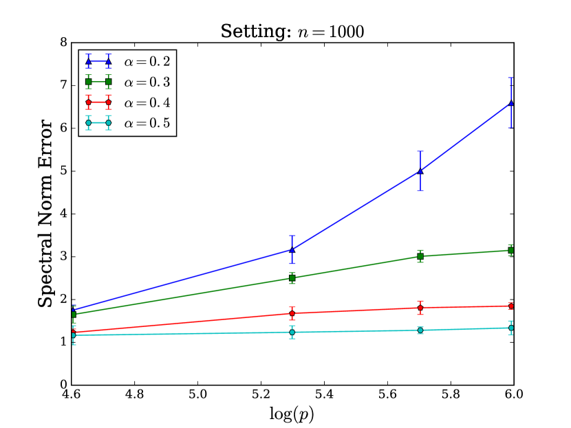
(a) Spectral norm error as $\log p$ changes.

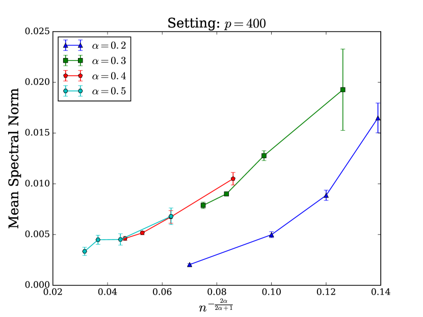
(b) Mean spectral norm error as $n^{-\frac{2\alpha}{2\alpha+1}}$ changes.

Figure 1: Experimental results. Note that the plotted error grows linearly as a function of $\log p$ and $n^{-\frac{2\alpha}{2\alpha+1}}$, respectively, matching the theoretical results; however, the linear relationship is less clear in the $\alpha=0.2$ case, due to the subtle interplay of the error terms.

5 Discussion

Theorems 3.1 and 3.2 together establish that the minimax rate of convergence for estimating precision matrices over the parameter space $\mathcal{F}_{\alpha}$ given in Equation (3) is $n^{-\frac{2\alpha}{2\alpha+1}}+\frac{\log p}{n}$. The theorems further imply that the blockwise estimator with $k=n^{\frac{1}{2\alpha+1}}$ achieves this optimal rate of convergence.

As in the bandable covariance case established by [6], we may observe that different regimes dictate which term dominates in the rate of convergence. In the setting where $\log p$ is of a lower order than $n^{\frac{1}{2\alpha+1}}$, the $n^{-\frac{2\alpha}{2\alpha+1}}$ term dominates, and the rate of convergence is determined by the smoothness parameter $\alpha$. However, when $\log p$ is much larger than $n^{\frac{1}{2\alpha+1}}$, $p$ has a much greater influence on the minimax rate of convergence.

Overall, we have shown how much performance gains can be obtained through added structural constraints. An interesting line of future work will be to explore algorithms that uniformly exhibit a smooth transition between fully banded models and sparse models on the precision matrix. Such methods could adapt to the structure and allow for mixtures between banded and sparse precision matrices. The results presented here apply to the case of subgaussian random variables. Unfortunately, moving away from the Gaussian setting in general breaks the connection between precision matrices and graph structure. Hence, a fruitful line of work will be to also develop methods that can be applied to general exponential families.

Acknowledgements

We would like to thank Harry Zhou for stimulating discussions regarding matrix estimation problems. SN acknowledges funding from NSF Grant DMS 1723128.

Appendix A Proof of Auxiliary Lemmas

We now present the proofs of the auxiliary lemmas presented above. The proofs of Lemmas 1 and 2 are closely related to the analogous proofs of [6]. For completeness, we adapt those proofs below.

A.1 Proof of Lemma 1

Consider a pair $i,j$, indexing an entry of $\Omega_{A}$. Without loss of generality, assume that $i\leq j$. Then, for a fixed $l,m$, the set $\{i,j\}$ is contained in $\{l,\dotsc,l+m-1\}$ if and only if $l\leq i\leq j\leq l+m-1$. This condition is equivalently stated as $j-m+1\leq l\leq i$.

Keeping $i,j,m$ fixed, $\operatorname{Card}\{l:j-m+1\leq l\leq i\}$ intuitively gives the number of $\Omega_{l}^{(m)}$ that are nonzero on the $ij^{\mathrm{th}}$ entry. Observe that:

$$\operatorname{Card}\{l:j-m+1\leq l\leq i\} =\left(i-(j-m+1)+1\right)_{+}$$

$$=\left(m-|i-j|\right)_{+}$$

It immediately follows that:

$$\operatorname{Card}\{l:j-k+1\leq l\leq i\} =\left(k-|i-j|\right)_{+}$$

$$\operatorname{Card}\{l:j-\nicefrac{{k}}{{2}}+1\leq l\leq i\} =\left(\nicefrac{{k}}{{2}}-|i-j|\right)_{+}$$

Therefore, the tapering coefficient may be expressed:

$$\frac{k}{2}\cdot v_{ij} =\left(k-|i-j|\right)_{+}-\left(\nicefrac{{k}}{{2}}-|i-j|\right)_{+}$$

$$=\operatorname{Card}\{l:j-k+1\leq l\leq i\}-\operatorname{Card}\{l:j-\nicefrac{{k}}{{2}}+1\leq l\leq i\}$$

∎

A.2 Proof of Lemma 2

By construction, we may decompose:

$$\left\lVert\hat{\Omega}_{m}-\Omega_{A}\right\rVert\leq\frac{2}{m}\cdot\left(\left\lVert\sum_{l=1-m}^{p}\hat{\Omega}_{l}^{(m)}-\Omega_{l}^{(m)}\right\rVert-\left\lVert\sum_{l=1-\nicefrac{{m}}{{2}}}^{p}\hat{\Omega}_{l}^{(\nicefrac{{m}}{{2}})}-\Omega_{l}^{(\nicefrac{{m}}{{2}})}\right\rVert\right)$$ (35)

Assume without loss of generality that $p$ is divisible by $m$. We may rewrite:

$$\left\lVert\sum_{l=1-m}^{p}\hat{\Omega}_{l}^{(m)}-\Omega_{l}^{(m)}\right\rVert =\left\lVert\sum_{j=-1}^{\nicefrac{{p}}{{m}}}\sum_{l=1}^{m}\hat{\Omega}_{jm+l}^{(m)}-\Omega_{jm+l}^{(m)}\right\rVert$$

$$\leq\sum_{l=1}^{m}\left\lVert\sum_{j=-1}^{\nicefrac{{p}}{{m}}}\hat{\Omega}_{jm+l}^{(m)}-\Omega_{jm+l}^{(m)}\right\rVert$$

$$\leq m\cdot\max_{1\leq l\leq m}\left\lVert\sum_{j=-1}^{\nicefrac{{p}}{{m}}}\hat{\Omega}_{jm+l}^{(m)}-\Omega_{jm+l}^{(m)}\right\rVert$$

Because $\hat{\Omega}_{jm+l}^{(m)},\Omega_{jm+l}^{(m)}$ are disjoint diagonal subblocks over $-1\leq j\leq\nicefrac{{p}}{{m}}$, it follows that:

$$\left\lVert\sum_{l=1-m}^{p}\hat{\Omega}_{l}^{(m)}-\Omega_{l}^{(m)}\right\rVert\leq m\cdot\max_{1-m\leq l\leq p}\left\lVert\hat{\Omega}_{jm+l}^{(m)}-\Omega_{jm+l}^{(m)}\right\rVert\\$$ (36)

Therefore, from Equations (35) and (36) we have:

$$\left\lVert\hat{\Omega}_{m}-\Omega_{A}\right\rVert \leq 2N^{(m)}+N^{(\nicefrac{{m}}{{2}})}$$

$$\leq C\cdot N^{(m)}$$

A.3 Proof of Lemma 3

Assume without loss of generality that $l\in[2m+1,p-3m]$. This argument can be extended to the periphery easily.

Consider a given $m\times m$ block of interest $\Omega_{l}^{(m)}$. We denote the $3m\times 3m$ block centered about $\Omega_{l}^{(m)}$ by $\Omega_{l-m}^{(3m)}$. We permute the rows and columns of $\Omega$ such that $\Omega_{l-m}^{(3m)}$ is located in the upper left. This permuted matrix may be expressed as:

$$\pi(\Omega) =\begin{bmatrix}\Omega_{l-m\leq i,j\leq p}&\Omega_{l-m\leq i\leq p,1\leq j<l-m}\\ \Omega_{l-m\leq i\leq p,1\leq j<l-m}^{\top}&\Omega_{1\leq i,j<l-m}\end{bmatrix}$$

$$=\begin{bmatrix}\Omega_{l-m}^{(3m)}&\Omega_{B}\\ \Omega_{B}^{\top}&\Omega_{C}\end{bmatrix}$$

Let us express:

$$\Omega_{B}=\begin{bmatrix}\Omega_{B_{1}}\\ \Omega_{B_{2}}\\ \Omega_{B_{3}}\end{bmatrix}$$

with $\Omega_{B_{2}}$ spanning the indices:

$$\Omega_{B_{2}}=\begin{bmatrix}\Omega_{l\leq i<l+m,l+2m\leq j\leq p}&\Omega_{l\leq i<l+m,1\leq j<l-m}\end{bmatrix}$$

By examining indices, we see that $\Omega_{B_{2}}$ has no entries within $m$ of the diagonal.

Now, consider $\Sigma=\pi(\Omega)^{-1}$. If we take the upper left $3m\times 3m$ block $\Sigma_{3m}$ of $\Sigma$ and invert it by the Schur complement, we obtain:

$$\Sigma_{3m}^{-1} =\Omega_{l-m}^{(3m)}-\Omega_{B}\Omega_{C}^{-1}\Omega_{B}^{\top}$$

At this point, we note that the central $m\times m$ block of $\Omega_{l-m}^{(3m)}$ is in fact $\Omega_{l}^{(m)}$, and denote the central $m\times m$ block of $\Sigma_{3m}^{-1}$ by $\tilde{\Omega}_{l}^{(m)}$. Therefore, we may write:

$$\tilde{\Omega}_{l}^{(m)} =\Omega_{l}^{(m)}-\Omega_{B_{2}}\Omega_{C}^{-1}\Omega_{B_{2}}^{\top}$$

∎

A.4 Proof of Lemma 4

Recall from Lemma 3 that $W=\Omega_{B_{2}}\Omega_{C}^{-1}\Omega_{B_{2}}^{\top}$, where $\Omega_{B_{2}}$ has no in-band entries. First, we bound, with $k=m$:

$$\left\lVert\Omega_{B_{2}}\right\rVert \leq\left\lVert\begin{bmatrix}0&\Omega_{B_{2}}\\ \Omega_{B_{2}}^{\top}&0\end{bmatrix}\right\rVert$$

$$\leq\left\lVert\Omega_{B_{2}}\right\rVert_{1}$$

$$\leq Mk^{-\alpha}$$

Next, we bound the spectral norm of $\Omega_{C}^{-1}$. Note that this is equivalent to bounding $\lambda_{\mathrm{min}}(\Omega_{C})$ away from zero.

$$\lambda_{\mathrm{min}}(\Omega_{C}) =\min_{\begin{subarray}{c}\tilde{\mathbf{v}}\in\mathbf{R}^{p-3m},\\ \left\lVert\tilde{\mathbf{v}}\right\rVert=1\end{subarray}}\left\lVert\Omega_{C}\tilde{\mathbf{v}}\right\rVert$$

$$=\min_{\begin{subarray}{c}\mathbf{v}\in\mathbf{R}^{p},\\ \left\lVert\mathbf{v}\right\rVert=1,\\ \mathbf{v}_{\operatorname{supp}(C)^{c}}=0\end{subarray}}\left\lVert\Omega\mathbf{v}\right\rVert$$

$$\geq\min_{\begin{subarray}{c}\mathbf{v}\in\mathbf{R}^{p},\\ \left\lVert\mathbf{v}\right\rVert=1\end{subarray}}\left\lVert\Omega\mathbf{v}\right\rVert$$

$$\geq\frac{1}{M_{0}}$$

Therefore, we may conclude:

$$\left\lVert W\right\rVert \leq\left\lVert\Omega_{B_{2}}\right\rVert^{2}\left\lVert\Omega_{C}^{-1}\right\rVert$$

$$\leq Cm^{-2\alpha}$$

∎

A.5 Proof of Lemma 5

Note that for arbitrary $l,m$, we have:

$$\left\lVert\hat{\Omega}_{l}^{(m)}-\tilde{\Omega}_{l}^{(m)}\right\rVert \leq\left\lVert\hat{\Omega}_{l-m}^{(3m)}-\tilde{\Omega}_{l-m}^{(3m)}\right\rVert$$

$$=\left\lVert\hat{\Sigma}_{3m}^{-1}-\Sigma_{3m}^{-1}\right\rVert$$

$$\leq\left\lVert\Sigma_{3m}^{-1}\right\rVert\left\lVert\Sigma_{3m}-\hat{\Sigma}_{3m}\right\rVert\left\lVert\hat{\Sigma}_{3m}^{-1}\right\rVert$$

We now consider the spectral norm of the matrix $\hat{\Sigma}_{3m}^{-1}$. We may bound the minimum eigenvalue of $\hat{\Sigma}_{3m}$ away from zero with high probability.

By decomposing $\hat{\Sigma}_{3m}=\Sigma_{3m}+(\hat{\Sigma}_{3m}-\Sigma_{3m})$ and applying Weyl’s Theorem [10]:

$$\lambda_{\mathrm{min}}(\hat{\Sigma}_{3m}) \geq\lambda_{\mathrm{min}}(\Sigma_{3m})+\lambda_{\mathrm{min}}(\hat{\Sigma}_{3m}-\Sigma_{3m})$$

$$\geq\lambda_{\mathrm{min}}(\Sigma_{3m})-\left\lVert\hat{\Sigma}_{3m}-\Sigma_{3m}\right\rVert$$

We now state a useful result for bounding the spectral norm of a random matrix.

Lemma 10.

Suppose $A$ is an $m\times n$ subgaussian random matrix. Then there exists some $\rho>0$ such that:

$$\mathbf{P}\left\{\left\lVert A\right\rVert>t\right\}\leq 5^{m+n}\exp\left\{-t^{2}\rho\right\}$$ (37)

Furthermore, let $\mathbf{x}_{1},\dotsc,\mathbf{x}_{n}\in\mathbf{R}^{m}$ be i.i.d. vectors with $\operatorname{\mathbf{E}}(\mathbf{x}_{i}-\mu)(\mathbf{x}_{i}-\mu)^{\top}=\Sigma$. Denote the empirical covariance matrix $\hat{\Sigma}=\frac{1}{n}\sum_{i=1}^{n}(\mathbf{x}_{i}-\bar{\mathbf{x}})(\mathbf{x}_{i}-\bar{\mathbf{x}})^{\top}$. Then for some $\tilde{\rho}>0$:

$$\mathbf{P}\left\{\left\lVert\hat{\Sigma}-\Sigma\right\rVert>x\right\}\leq{25}^{m}\exp\left\{-\frac{nx^{2}\tilde{\rho}}{2}\right\}+5^{m}\exp\left\{-\frac{nx\tilde{\rho}}{2}\right\}$$ (38)

for all $0<x<\tilde{\rho}$.

By the above result there exists some $\tilde{\rho}>0$ such that:

$$\mathbf{P}\left\{\left\lVert\Sigma_{3m}-\hat{\Sigma}_{3m}\right\rVert>x\right\} \leq{25}^{3m}\exp\left\{-\frac{nx^{2}\tilde{\rho}}{2}\right\}\,+\,5^{3m}\exp\left\{-\frac{nx\tilde{\rho}}{2}\right\}$$

for all $0<x<\tilde{\rho}$. Choose $x=2\sqrt{\frac{m+\log p}{n\tilde{\rho}}}$ and note that $x=o(1)$, by our assumptions. Thus,

$$\mathbf{P}\left\{\left\lVert\Sigma_{3m}-\hat{\Sigma}_{3m}\right\rVert>2\sqrt{\frac{m+\log p}{n\tilde{\rho}}}\right\} =O\left(p^{-4}\right)$$

Assume $n\rho_{1}>4M_{0}^{2}(m+\log p)$. Then, with high probability, we have:

$$\lambda_{\mathrm{min}}(\hat{\Sigma}_{3m}) \geq\lambda_{\mathrm{min}}(\Sigma_{3m})-2\cdot\frac{1}{2M_{0}}$$

$$=\lambda_{\mathrm{min}}(\Sigma_{3m})-\frac{1}{2M_{0}}$$

$$=\lambda_{\mathrm{min}}(\Sigma_{3m})-\frac{1}{2}\lambda_{\mathrm{min}}(\Sigma_{3m})$$

$$=\frac{1}{2}M_{0}>c>0$$

Therefore, it follows that:

$$\left\lVert\hat{\Omega}_{l}^{(m)}-\tilde{\Omega}_{l}^{(m)}\right\rVert \leq C\left\lVert\Sigma_{3m}-\hat{\Sigma}_{3m}\right\rVert$$

with high probability. We now re-apply the concentration bound from Lemma 10. There exists a constant $\rho_{1}>0$ such that:

$$\mathbf{P}\left\{\left\lVert\hat{\Omega}_{l}^{(m)}-\tilde{\Omega}_{l}^{(m)}\right\rVert>Cx\right\} =\mathbf{P}\left\{\left\lVert\Sigma_{3m}-\hat{\Sigma}_{3m}\right\rVert>x\right\}$$

$$\leq{25}^{3m}\exp\left\{-nx^{2}\rho_{1}\right\}$$

Then, by the union bound, we have:

$$\mathbf{P}\left\{\max_{1\leq l\leq p-m+1}\left\lVert\hat{\Omega}_{l}^{(m)}-\tilde{\Omega}_{l}^{(m)}\right\rVert>Cx\right\} \leq\sum_{1\leq l\leq p-m+1}\mathbf{P}\left\{\left\lVert\hat{\Omega}_{l}^{(m)}-\tilde{\Omega}_{l}^{(m)}\right\rVert>Cx\right\}$$

$$\leq 2p\cdot{25}^{3m}\exp\left\{-nx^{2}\rho_{1}\right\}$$

∎

A.6 Proof of Lemma 6

Let $\Omega(\theta)\in\mathcal{F}_{11}$ be defined as in Equation (24). We wish to show that:

$$\min_{H(\theta,\theta^{\prime})\geq 1}\frac{\left\lVert\Omega(\theta)-\Omega(\theta^{\prime})\right\rVert^{2}}{H(\theta,\theta^{\prime})}\geq cka^{2}$$

Define $v=(\mathbf{1}\{k\leq i\leq 2k\})_{i}\in\mathbf{R}^{p}$, $w=[\Omega(\theta)-\Omega(\theta^{\prime})]v$. Observe that there are exactly $H(\theta,\theta^{\prime})$ entries in $w$ such that $|w_{i}|=\tau ka$. Further note that $\left\lVert v\right\rVert_{2}^{2}=k$. This implies:

$$\left\lVert\Omega(\theta)-\Omega(\theta^{\prime})\right\rVert^{2} \geq\frac{\left\lVert[\Omega(\theta)-\Omega(\theta^{\prime})]v\right\rVert_{2}^{2}}{\left\lVert v\right\rVert_{2}^{2}}$$

$$\geq\frac{H(\theta,\theta^{\prime})\cdot(\tau ka)^{2}}{k}$$

$$=H(\theta,\theta^{\prime})\tau^{2}ka^{2}$$

It then follows that:

$$\frac{\left\lVert\Omega(\theta)-\Omega(\theta^{\prime})\right\rVert^{2}}{H(\theta,\theta^{\prime})} \geq\tau^{2}ka^{2}$$

$$\Rightarrow\min_{H(\theta,\theta^{\prime})\geq 1}\frac{\left\lVert\Omega(\theta)-\Omega(\theta^{\prime})\right\rVert^{2}}{H(\theta,\theta^{\prime})} \geq cka^{2}$$

∎

A.7 Proof of Lemma 7

Let $\mathbf{x}_{1},\dotsc,\mathbf{x}_{n}\stackrel{{\scriptstyle\mathrm{iid}}}{{\sim}}\mathcal{N}(\Omega(\theta))$ with $\Omega(\theta)\in\mathcal{F}_{11}$ as defined in Equation (24), with joint distribution $\mathbf{P}_{\theta}$. We wish to show that for some constant $c>0$:

$$\min_{H(\theta,\theta^{\prime})=1}\left\lVert\mathbf{P}_{\theta}\wedge\mathbf{P}_{\theta^{\prime}}\right\rVert\geq c$$

Because $\left\lVert\mathbf{P}_{1}\wedge\mathbf{P}_{2}\right\rVert=1-\frac{1}{2}\left\lVert\mathbf{P}_{1}-\mathbf{P}_{2}\right\rVert_{1}$, it is sufficient to show that:

$$\left\lVert\mathbf{P}_{\theta}-\mathbf{P}_{\theta^{\prime}}\right\rVert_{1}^{2}\leq c$$

We may bound the squared $\ell_{1}$-norm from above by the Kullback-Leibler Divergence:

$$\left\lVert\mathbf{P}_{\theta}-\mathbf{P}_{\theta^{\prime}}\right\rVert_{1}^{2} \leq 2D_{\mathrm{KL}}(\mathbf{P}_{\theta}|\mathbf{P}_{\theta^{\prime}})$$

$$=2n\left[\frac{1}{2}\operatorname{\mathrm{tr}}\left(\Omega^{-1}(\theta^{\prime})\Omega(\theta)\right)-\frac{1}{2}\log\det\left(\Omega^{-1}(\theta^{\prime})\Omega(\theta)\right)-\frac{p}{2}\right]$$

This reduced form of the Kullback-Leibler Divergence is a consequence of the zero mean for the distribution of $\mathbf{P}_{\theta},\mathbf{P}_{\theta^{\prime}}$. We will show that we may bound this quantity from above by a constant.

First, we define $D_{1}\triangleq\Omega(\theta)-\Omega(\theta^{\prime})$. Observe that:

$$\Omega^{-1}(\theta^{\prime})D_{1} =\Omega^{-1}(\theta^{\prime})\Omega(\theta)-\mathbf{I}_{p}$$

$$\Leftrightarrow\Omega^{-1}\Omega(\theta) =\Omega^{-1}(\theta^{\prime})D_{1}+\mathbf{I}_{p}$$

From these identities, we may rewrite:

$$\frac{1}{2}\operatorname{\mathrm{tr}}\left(\Omega^{-1}(\theta^{\prime})\Omega(\theta)\right)-\frac{p}{2} =\frac{1}{2}\operatorname{\mathrm{tr}}\left(\Omega^{-1}(\theta^{\prime})D_{1}\right)$$

Denote the eigenvalues of $\Omega^{-1}(\theta^{\prime})D_{1}$ by $\lambda_{i}$. Then:

$$\operatorname{\mathrm{tr}}\left(\Omega^{-1}(\theta^{\prime})D_{1}\right) =\sum_{i=1}^{p}\lambda_{i}$$

We may then bound the spectrum of $\Omega^{-1}(\theta^{\prime})D_{1}$ by bounding the spectrum of the similar matrix $\Omega^{-\frac{1}{2}}(\theta^{\prime})D_{1}\Omega^{-\frac{1}{2}}(\theta^{\prime})$:

$$\left\lVert\Omega^{-1}(\theta^{\prime})D_{1}\right\rVert =\left\lVert\Omega^{-\frac{1}{2}}(\theta^{\prime})D_{1}\Omega^{-\frac{1}{2}}(\theta^{\prime})\right\rVert$$

$$\leq\left\lVert\Omega^{-\frac{1}{2}}\right\rVert\left\lVert D_{1}\right\rVert\left\lVert\Omega^{-\frac{1}{2}}\right\rVert$$

$$\leq c_{1}\left\lVert D_{1}\right\rVert$$

$$\leq c_{1}\left\lVert D_{1}\right\rVert_{1}$$

$$\leq c_{2}ka$$

where $\left\lVert A\right\rVert_{1}=\max_{j}\left\lVert A_{.j}\right\rVert_{1}$ denotes the matrix $\ell_{1}$ norm. This bound on the spectrum implies that $\lambda_{i}\in[-c_{2}ka,c_{2}ka]$, with $ka=k^{-\alpha}=n^{-\frac{\alpha}{2\alpha+1}}\rightarrow 0$.

Now, we bound the $\log\det\left(\Omega^{-1}(\theta^{\prime})\Omega(\theta)\right)$ term:

$$\log\det\left(\Omega^{-1}(\theta^{\prime})\Omega(\theta)\right) =\log\det\left(\mathbf{I}_{p}+\Omega^{-1}(\theta^{\prime})D_{1}\right)$$

$$=\sum_{i=1}^{p}\log(1+\lambda_{i})$$

$$=\sum_{i=1}^{p}\lambda_{i}+\left(\log(1+\lambda_{i})-\lambda_{i}\right)$$

$$\geq\operatorname{\mathrm{tr}}\left(\Omega^{-1}(\theta^{\prime})D_{1}\right)+\sum_{i=1}^{p}\left[\frac{\lambda_{i}}{1+\lambda_{i}}-\frac{\lambda_{i}+\lambda_{i}^{2}}{1+\lambda_{i}}\right]$$

$$=\operatorname{\mathrm{tr}}\left(\Omega^{-1}(\theta^{\prime})D_{1}\right)-\sum_{i=1}^{p}\frac{\lambda_{i}^{2}}{1+\lambda_{i}}$$

$$\geq\operatorname{\mathrm{tr}}\left(\Omega^{-1}(\theta^{\prime})D_{1}\right)-c_{3}\sum_{i=1}^{p}\lambda_{i}^{2}$$

where we may bound:

$$\sum_{i=1}^{p}\lambda_{i}^{2} =\left\lVert\Omega^{-1}(\theta^{\prime})D_{1}\right\rVert_{F}^{2}$$

$$=\left\lVert\Omega^{-\frac{1}{2}}(\theta^{\prime})D_{1}\Omega^{-\frac{1}{2}}(\theta^{\prime})\right\rVert_{F}^{2}$$

$$\leq\left\lVert\Omega^{-\frac{1}{2}}(\theta^{\prime})\right\rVert^{2}\left\lVert D_{1}\right\rVert_{F}^{2}\left\lVert\Omega^{-\frac{1}{2}}(\theta^{\prime})\right\rVert^{2}$$

$$\leq c_{4}ka^{2}$$

due to $H(\theta,\theta^{\prime})=1$. This in turn implies that:

$$\log\det\left(\Omega^{-1}(\theta^{\prime})\Omega(\theta)\right) \geq\operatorname{\mathrm{tr}}\left(\Omega^{-1}(\theta^{\prime})D_{1}\right)-c_{3}\sum_{i=1}^{p}\lambda_{i}^{2}$$

$$\geq\operatorname{\mathrm{tr}}\left(\Omega^{-1}(\theta^{\prime})D_{1}\right)-c_{5}ka^{2}$$

$$\Rightarrow-\frac{1}{2}\log\det\left(\Omega^{-1}(\theta^{\prime})\Omega(\theta)\right) \leq-\frac{1}{2}\operatorname{\mathrm{tr}}\left(\Omega^{-1}(\theta^{\prime})D_{1}\right)+\frac{c_{5}}{2}ka^{2}$$

Finally, this results in the bound:

$$\left\lVert\mathbf{P}_{\theta}-\mathbf{P}_{\theta^{\prime}}\right\rVert_{1}^{2} \leq 2n\left[\frac{1}{2}\operatorname{\mathrm{tr}}\left(\Omega^{-1}(\theta^{\prime})D_{1}\right)-\frac{1}{2}\log\det\left(\Omega^{-1}(\theta^{\prime})\Omega(\theta)\right)\right]$$

$$\leq 2n\cdot\frac{c_{5}}{2}ka^{2}$$

$$=c_{5}nka^{2}$$

$$=c_{5}nk^{-2\alpha-1}$$

$$=c_{5}\cdot n\cdot n^{-\frac{2\alpha+1}{2\alpha+1}}$$

$$=c_{5}$$

This immediately implies that:

$$\left\lVert\mathbf{P}_{\theta}\wedge\mathbf{P}_{\theta^{\prime}}\right\rVert\geq c>0$$

∎

A.8 Proof of Lemma 8

We can directly evaluate, for all $j,m$:

$$\int\frac{f_{j}f_{m}}{f_{0}}d\mu =\int\frac{\prod_{\begin{subarray}{c}1\leq i\leq n\\ 1\leq k\leq p_{1}\\ k\neq j\end{subarray}}\phi_{1}(x_{k}^{i})\prod_{\begin{subarray}{c}1\leq i\leq n\\ 1\leq k\leq p_{1}\\ k\neq m\end{subarray}}\phi_{1}(x_{k}^{i})\prod_{1\leq i\leq n}\phi_{\sigma_{mm}}(x_{m}^{i})\phi_{\sigma_{mm}}(x_{j}^{i})}{\prod_{\begin{subarray}{c}1\leq i\leq n\\ 1\leq k\leq p_{1}\end{subarray}}\phi_{1}(x_{k}^{i})}d\left\{x_{k}^{i}\right\}_{\begin{subarray}{c}1\leq i\leq n\\ 1\leq k\leq p_{1}\end{subarray}}$$

(Independence.)

$$=\prod_{1\leq i\leq n}\int\frac{\left[\prod_{\begin{subarray}{c}1\leq k\leq p_{1}\\ k\neq j\end{subarray}}\phi_{1}(x_{k}^{i})\right]\left[\prod_{\begin{subarray}{c}1\leq k\leq p_{1}\\ k\neq m\end{subarray}}\phi_{1}(x_{k}^{i})\right]\phi_{\sigma_{mm}}(x_{m}^{i})\phi_{\sigma_{mm}}(x_{j}^{i})}{\prod_{1\leq k\leq p_{1}}\phi_{1}(x_{k}^{i})}d\left\{x_{k}^{i}\right\}_{1\leq k\leq p_{1}}$$

$$=\prod_{1\leq i\leq n}\int\left[\prod_{\begin{subarray}{c}1\leq k\leq p_{1}\\ k\not\in\{j,m\}\end{subarray}}\phi_{1}(x_{k}^{i})\right]\phi_{\sigma_{mm}}(x_{m}^{i})\phi_{\sigma_{mm}}(x_{j}^{i})d\left\{x_{k}^{i}\right\}_{1\leq k\leq p_{1}}$$

(Independence.)

$$=\prod_{1\leq i\leq n}\left[\left[\prod_{\begin{subarray}{c}1\leq k\leq p_{1}\\ k\not\in\{j,m\}\end{subarray}}\int\phi_{1}(x_{k}^{i})dx_{k}^{i}\right]\int\phi_{\sigma_{mm}}(x_{m}^{i})dx_{m}^{i}\int\phi_{\sigma_{mm}}(x_{j}^{i})dx_{j}^{i}\right]$$

$$=\prod_{1\leq i\leq n}1$$

$$=1$$

∎

A.9 Proof of Lemma 9

For the squared terms:

$$\int\frac{f_{m}^{2}}{f_{0}}d\mu =\int\frac{\prod_{\begin{subarray}{c}1\leq i\leq n\\ 1\leq j\leq p_{1}\\ j\neq m\end{subarray}}\phi_{1}(x_{j}^{i})^{2}\prod_{1\leq i\leq n}\phi_{\sigma_{mm}}(x_{m}^{i})^{2}}{\prod_{\begin{subarray}{c}1\leq i\leq n\\ 1\leq j\leq p_{1}\end{subarray}}\phi_{1}(x_{j}^{i})}d\left\{x_{j}^{i}\right\}_{\begin{subarray}{c}1\leq i\leq n\\ 1\leq j\leq p_{1}\end{subarray}}$$

(Independence.)

$$=\prod_{1\leq i\leq n}\int\frac{\left[\prod_{\begin{subarray}{c}1\leq j\leq p_{1}\\ j\neq m\end{subarray}}\phi_{1}(x_{j}^{i})^{2}\right]\phi_{\sigma_{mm}}(x_{m}^{i})^{2}}{\prod_{1\leq j\leq p_{1}}\phi_{1}(x_{j}^{i})}d\left\{x_{j}^{i}\right\}_{1\leq j\leq p_{1}}$$

$$=\prod_{1\leq i\leq n}\int\frac{\left[\prod_{\begin{subarray}{c}1\leq j\leq p_{1}\\ j\neq m\end{subarray}}\phi_{1}(x_{j}^{i})\right]\phi_{\sigma_{mm}}(x_{m}^{i})^{2}}{\phi_{1}(x_{m}^{i})}d\left\{x_{j}^{i}\right\}_{1\leq j\leq p_{1}}$$

$$=\prod_{1\leq i\leq n}\left[\prod_{\begin{subarray}{c}1\leq j\leq p_{1}\\ j\neq m\end{subarray}}\int\phi_{1}(x_{j}^{i})dx_{j}^{i}\right]\int\frac{\phi_{\sigma_{mm}}(x_{m}^{i})^{2}}{\phi_{1}(x_{m}^{i})}dx_{m}^{i}$$

$$=\prod_{1\leq i\leq n}\int\frac{\phi_{\sigma_{mm}}(x_{m}^{i})^{2}}{\phi_{1}(x_{m}^{i})}dx_{m}^{i}$$

We now substitute in the form of the density functions and move the normalization terms out of the integral:

$$\prod_{1\leq i\leq n}\int\frac{\phi_{\sigma_{mm}}(x_{m}^{i})^{2}}{\phi_{1}(x_{m}^{i})}dx_{m}^{i} =\frac{(\sqrt{2\pi\sigma_{mm}})^{-2n}}{(\sqrt{2\pi})^{-n}}\prod_{1\leq i\leq n}\int\exp\left\{-2\cdot\frac{(x_{m}^{i})^{2}}{2\sigma_{mm}}\right\}\exp\left\{\frac{(x_{m}^{i})^{2}}{2}\right\}$$

$$=\frac{(\sqrt{2\pi\sigma_{mm}})^{-2n}}{(\sqrt{2\pi})^{-n}}\prod_{1\leq i\leq n}\int\exp\left\{-\frac{1}{2}\left[\frac{(x_{m}^{i})^{2}}{\frac{\sigma_{mm}}{2-\sigma_{mm}}}\right]\right\}$$

$$=\frac{(\sqrt{2\pi\sigma_{mm}})^{-2n}}{(\sqrt{2\pi})^{-n}}\left(\frac{2\pi\sigma_{mm}}{2-\sigma_{mm}}\right)^{\frac{n}{2}}$$

$$=(\sqrt{\sigma_{mm}})^{-2n}\left(\frac{\sigma_{mm}}{2-\sigma_{mm}}\right)^{\frac{n}{2}}$$

$$=(\sqrt{\sigma_{mm}})^{-n}(\sqrt{2-\sigma_{mm}})^{-n}$$

$$=\left[2\sigma_{mm}-\sigma_{mm}^{2}\right]^{-\frac{n}{2}}$$

$$=\left[1-(1-\sigma_{mm})^{2}\right]^{-\frac{n}{2}}$$

$$=\left(1-\tau\frac{\log p_{1}}{n}\right)^{-\frac{n}{2}}$$

∎

A.10 Proof of Lemma 10

We proceed with an $\epsilon$-net argument. The proof is done in the case $m=n$, and the extension to the general case is immediate. Let $S^{m-1}$ denote the $\ell_{2}$-sphere in $\mathbf{R}^{m}$, and let $S_{\nicefrac{{1}}{{2}}}^{m-1}$ be a $\nicefrac{{1}}{{2}}$-net of $S^{m-1}$. Note that for every $\mathbf{u}\in S^{m-1}$, there exists $\mathbf{x}\in S_{\nicefrac{{1}}{{2}}}^{m-1}$, $\mathbf{v}\in\mathbf{R}^{m}:\left\lVert v\right\rVert\leq\nicefrac{{1}}{{2}}$ such that $\mathbf{u}=\mathbf{x}+\mathbf{v}$. Then, for any matrix $A\in\mathbf{R}^{m\times m}$, we may discretize the sphere $S^{m-1}$:

$$\left\lVert A\right\rVert =\sup_{\mathbf{u}\in S^{m-1}}\left\lVert A\mathbf{u}\right\rVert$$

$$\leq\sup_{\mathbf{x}\in S_{\nicefrac{{1}}{{2}}}^{m-1}}\left\lVert A\mathbf{x}\right\rVert+\sup_{\mathbf{v}:\left\lVert\mathbf{v}\right\rVert\leq\frac{1}{2}}\left\lVert A\mathbf{v}\right\rVert$$

$$\leq\sup_{\mathbf{x}\in S_{\nicefrac{{1}}{{2}}}^{m-1}}\left\lVert A\mathbf{x}\right\rVert+\frac{1}{2}\left\lVert A\right\rVert$$

$$\Rightarrow\left\lVert A\right\rVert \leq 2\sup_{\mathbf{x}\in S_{\nicefrac{{1}}{{2}}}^{m-1}}\left\lVert A\mathbf{x}\right\rVert$$

Following a similar line of reasoning:

$$\left\lVert A\mathbf{x}\right\rVert =\sup_{\mathbf{y}\in S^{m-1}}\langle A\mathbf{x},\mathbf{y}\rangle$$

$$\leq 2\sup_{\mathbf{y}\in S_{\nicefrac{{1}}{{2}}}^{m-1}}\langle A\mathbf{x},\mathbf{y}\rangle$$

Then, by symmetry, we have:

$$\left\lVert A\right\rVert \leq 4\sup_{\mathbf{x},\mathbf{y}\in S_{\nicefrac{{1}}{{2}}}^{m-1}}|\mathbf{x}^{\top}A\mathbf{y}|$$

From packing arguments, we have that the cardinality of $S_{\nicefrac{{1}}{{2}}}^{m-1}$ is at most $5^{m}$. Therefore, there exist $\mathbf{v}_{1},\dotsc,\mathbf{v}_{5^{m}}\in S^{m-1}$ such that for all $A\in\mathbf{R}^{m\times m}$,

$$\left\lVert A\right\rVert\leq 4\max_{i,j\leq 5^{m}}|\mathbf{v}_{i}^{\top}A\mathbf{v}_{j}|$$

Recall that all entries of the matrix $A$ are subgaussian with mean zero. Now, we note each entry of the vector $A\mathbf{v}_{j}$ is the result of an inner product between $A_{i.}$ and a unit vector $\mathbf{v}_{j}\in S_{\nicefrac{{1}}{{2}}}^{m-1}\subset S^{m-1}$; therefore, the entries of $A\mathbf{v}_{j}$ are also subgaussian distributed. We repeat this argument to note that $\mathbf{v}_{j}^{\top}A\mathbf{v}_{j}$ is subgaussian distributed for all $i,j$. Therefore, we may observe that:

$$\mathbf{P}\left\{\left\lVert A\right\rVert\geq t\right\} \leq\mathbf{P}\left\{\max_{i,j\leq 5^{m}}|\mathbf{v}_{i}^{\top}A\mathbf{v}_{j}|\geq\frac{t}{4}\right\}$$

$$\leq\sum_{i,j\leq 5^{m}}\mathbf{P}\left\{|\mathbf{v}_{i}^{\top}A\mathbf{v}_{j}|\geq\frac{t}{4}\right\}$$

$$\leq{25}^{m}\max_{i,j\leq 5^{m}}\mathbf{P}\left\{|\mathbf{v}_{j}^{\top}A\mathbf{v}_{j}|\geq\frac{t}{4}\right\}$$

$$\leq{25}^{m}\exp\left\{-t^{2}\rho\right\}$$

for some $\rho>0$, by the definition of subgaussianity. This proves (37). We now apply this result to show (38).

Recall that we have drawn $\mathbf{x}_{1},\dotsc,\mathbf{x}_{n}\in\mathbf{R}^{m}$ from a subgaussian distribution with population covariance $\Sigma$. We wish to bound $\left\lVert\hat{\Sigma}-\Sigma\right\rVert$ where $\hat{\Sigma}=\frac{1}{n}\sum_{i=1}^{n}(\mathbf{x}_{i}-\bar{\mathbf{x}})(\mathbf{x}_{i}-\bar{\mathbf{x}})^{\top}$. We may subtract the mean $\mu$ from both terms, yielding $\hat{\Sigma}=\frac{1}{n}\sum_{i=1}^{n}((\mathbf{x}_{i}-\mu)-(\bar{\mathbf{x}}-\mu))((\mathbf{x}_{i}-\mu)-(\bar{\mathbf{x}}-\mu))^{\top}$, which can be further simplified to

$$\hat{\Sigma}=\frac{1}{n}\sum_{i=1}^{n}(\mathbf{x}_{i}-\mu)(\mathbf{x}_{i}-\mu)^{\top}-(\bar{\mathbf{x}}-\mu)(\bar{\mathbf{x}}-\mu)^{\top}$$

Hence,

$$\left\lVert\hat{\Sigma}-\Sigma\right\rVert \leq\left\lVert\frac{1}{n}\sum_{i=1}^{n}(\mathbf{x}_{i}-\mu)(\mathbf{x}_{i}-\mu)^{\top}-\Sigma\right\rVert+\left\lVert(\bar{\mathbf{x}}-\mu)(\bar{\mathbf{x}}-\mu)^{\top}\right\rVert$$

$$=\left\lVert\frac{1}{n}\sum_{i=1}^{n}(\mathbf{x}_{i}-\mu)(\mathbf{x}_{i}-\mu)^{\top}-\Sigma\right\rVert+\|\bar{\mathbf{x}}-\mu\|_{2}^{2}$$

Thus,

$$\mathbf{P}\left\{\left\lVert\hat{\Sigma}-\Sigma\right\rVert\geq x\right\}\leq\mathbf{P}\left\{\|\bar{\mathbf{x}}-\mu\|_{2}^{2}\geq\frac{x}{2}\right\}+\mathbf{P}\left\{\left\lVert\frac{1}{n}\sum_{i=1}^{n}(\mathbf{x}_{i}-\mu)(\mathbf{x}_{i}-\mu)^{\top}-\Sigma\right\rVert\geq\frac{x}{2}\right\}$$

The first term is simply bounded by $5^{m}\exp\left\{-nx\rho/2\right\}$ via an application of equation (37).

We next bound the second term. By (9), there exists a $\rho^{\prime}>0$ such that:

$$\mathbf{P}\left\{\mathbf{v}^{\top}(\mathbf{x}_{i}-\operatorname{\mathbf{E}}\mathbf{x}_{i})(\mathbf{x}_{i}-\operatorname{\mathbf{E}}\mathbf{x}_{i})^{\top}\mathbf{v}>x\right\}\leq\exp\left\{-\frac{x\rho^{\prime}}{2}\right\}$$

It follows that $\operatorname{\mathbf{E}}\exp\left(t\mathbf{v}^{\top}(\mathbf{x}_{i}-\operatorname{\mathbf{E}}\mathbf{x}_{i})(\mathbf{x}_{i}-\operatorname{\mathbf{E}}\mathbf{x}_{i})^{\top}\mathbf{v}\right)<\infty$ for all $t<\frac{\rho^{\prime}}{2}$ and $\left\lVert\mathbf{v}\right\rVert=1$. Then, there exists a $\tilde{\rho}$ such that:

$$\mathbf{P}\left\{\left|\frac{1}{n}\sum_{i=1}^{n}\mathbf{v}^{\top}[(\mathbf{x}_{i}-\operatorname{\mathbf{E}}\mathbf{x}_{i})(\mathbf{x}_{i}-\operatorname{\mathbf{E}}\mathbf{x}_{i})^{\top}-\Sigma]\mathbf{v}\right|>\frac{x}{2}\right\}\leq\exp\left\{-\frac{nx^{2}\tilde{\rho}}{4}\right\}$$

for all $0<x<\tilde{\rho}$ and $\left\lVert\mathbf{v}\right\rVert=1$. Thus (38) follows immediately from (37) and the above bound on the $\mathbf{P}\left\{\|\bar{\mathbf{x}}-\mu\|_{2}^{2}\geq\frac{x}{2}\right\}$. ∎

References

- [1] P. J. Bickel and Y. R. Gel. Banded regularization of autocovariance matrices in application to parameter estimation and forecasting of time series. Journal of the Royal Statistical Society: Series B (Statistical Methodology), 73(5):711–728, 2011.
- [2] S. Boyd and L. Vandenberghe. Convex optimization. Cambridge University Press, Cambridge, UK, 2004.
- [3] T. T. Cai, W. Liu, and X. Luo. A Constrained L1 Minimization Approach to Sparse Precision Matrix Estimation. arXiv:1102.2233 [stat], February 2011. arXiv: 1102.2233.
- [4] T. T. Cai, W. Liu, and H. H. Zhou. Estimating sparse precision matrix: Optimal rates of convergence and adaptive estimation. Ann. Statist., 44(2):455–488, 04 2016.
- [5] T. T. Cai, Z. Ren, H. H. Zhou, et al. Estimating structured high-dimensional covariance and precision matrices: Optimal rates and adaptive estimation. Electronic Journal of Statistics, 10(1):1–59, 2016.
- [6] T. T. Cai, C.-H. Zhang, and H. H. Zhou. Optimal rates of convergence for covariance matrix estimation. The Annals of Statistics, 38(4):2118–2144, August 2010.
- [7] T. T. Cai and H. H. Zhou. Optimal rates of convergence for sparse covariance matrix estimation. Ann. Statist., 40(5):2389–2420, 10 2012.
- [8] J. Friedman, T. Hastie, and R. Tibshirani. Sparse inverse covariance estimation with the graphical Lasso. Biostatistics, 2007.
- [9] K. J. Friston, P. Jezzard, and R. Turner. Analysis of functional mri time-series. Human brain mapping, 1(2):153–171, 1994.
- [10] R. A. Horn and C. R. Johnson. Matrix Analysis. Cambridge University Press, October 2012.
- [11] M. J. Hosseini and S.-I. Lee. Learning sparse gaussian graphical models with overlapping blocks. In Advances in Neural Information Processing Systems, pages 3808–3816, 2016.
- [12] S. L. Lauritzen. Graphical Models. Oxford Statistical Science Series. Clarendon Press, Oxford, 1996.
- [13] K. Lee and J. Lee. Estimating Large Precision Matrices via Modified Cholesky Decomposition. arXiv:1707.01143 [stat], July 2017. arXiv: 1707.01143.
- [14] N. Meinshausen and P. Bühlmann. High-dimensional graphs and variable selection with the Lasso. Annals of Statistics, 34:1436–1462, 2006.
- [15] N. Padmanabhan, M. White, H. H. Zhou, and R. O’Connell. Estimating sparse precision matrices. Monthly Notices of the Royal Astronomical Society, 460(2):1567–1576, 2016.
- [16] Z. Ren, T. Sun, C.-H. Zhang, and H. H. Zhou. Asymptotic normality and optimalities in estimation of large Gaussian graphical models. The Annals of Statistics, 43(3):991–1026, June 2015.
- [17] A. J. Rothman, P. J. Bickel, E. Levina, and J. Zhu. Sparse permutation invariant covariance estimation. Electronic Journal of Statistics, 2:494–515, 2008.
- [18] G. Saon and J. T. Chien. Bayesian sensing hidden markov models for speech recognition. In 2011 IEEE International Conference on Acoustics, Speech and Signal Processing (ICASSP), pages 5056–5059, May 2011.
- [19] A. B. Tsybakov. Introduction to Nonparametric Estimation. Springer Publishing Company, Incorporated, 1st edition, 2008.
- [20] H. Visser and J. Molenaar. Trend estimation and regression analysis in climatological time series: an application of structural time series models and the kalman filter. Journal of Climate, 8(5):969–979, 1995.
- [21] M. A. Woodbury. Inverting modified matrices. Statistical Research Group, Memo. Rep. no. 42. Princeton University, Princeton, N. J., 1950.
- [22] B. Yu. Assouad, Fano and Le Cam. In Festschrift for Lucien Le Cam, pages 423–435. Springer-Verlag, Berlin, 1997.
- [23] M. Yuan and Y. Lin. Model selection and estimation in the Gaussian graphical model. Biometrika, 94(1):19–35, 2007.