Protein Folding Optimization using Differential Evolution Extended with Local Search and Component Reinitialization

Abstract

This paper presents a novel Differential Evolution algorithm for protein folding optimization that is applied to a three-dimensional AB off-lattice model. The proposed algorithm includes two new mechanisms. A local search is used to improve convergence speed and to reduce the runtime complexity of the energy calculation. For this purpose, a local movement is introduced within the local search. The designed evolutionary algorithm has fast convergence speed and, therefore, when it is trapped into the local optimum or a relatively good solution is located, it is hard to locate a better similar solution. The similar solution is different from the good solution in only a few components. A component reinitialization method is designed to mitigate this problem. Both the new mechanisms and the proposed algorithm were analyzed on well-known amino acid sequences that are used frequently in the literature. Experimental results show that the employed new mechanisms improve the efficiency of our algorithm and that the proposed algorithm is superior to other state-of-the-art algorithms. It obtained a hit ratio of 100% for sequences up to 18 monomers, within a budget of $10^{11}$ solution evaluations. New best-known solutions were obtained for most of the sequences. The existence of the symmetric best-known solutions is also demonstrated in the paper.

1 Introduction

The protein structure prediction represents the problem of how to predict the native structure of a protein from its amino acid sequence. This problem is one of the more important challenges of this century Kennedy05 and, because of its nature, it attracts scientists from different fields, such as Physics, Chemistry, Biology, Mathematics, and Computer Science. Within the protein structure prediction, the Protein Folding Optimization (PFO) represents a computational problem for simulating the protein folding process and finding a native structure. Most proteins must fold into a unique three-dimensional structure, known as a native structure, to perform their biological function Balchin16 . A protein’s function is determined by its structure. The inability of a protein to form its native structure prevents a protein from fulfilling its function correctly, and this may be the basis of various human diseases Alfonso15 .

The PFO belongs to the class of NP-hard problems Fraenkel93 and, with current algorithms and computational resources, it is possible to predict the native structures of relatively small proteins. The reason for that is the huge and multimodal search space. For example, a polypeptide that has only 18 amino acids, will have 31 angles within a simplified AB model (see Section 3). Using uniform discretization with only 10 values for each angle, there would be $10^{31}$ possible configurations. To evaluate and select the correctly folded conformation among all these conformations in the time elapsed since the Big Bang, we need the huge computational speed of $10^{31}/(4.32\cdot 10^{17})=2.31\cdot 10^{13}$ conformation evaluations per second. This is much faster than the speed obtained within our experiment, where we can evaluate only $5.73\cdot 10^{5}$ conformations per second. From these numbers, we can see that the search space is huge, even in the simplified model, which makes this problem very hard. However, in reality, the proteins fold into their native conformation on a time scale of seconds, and this contradiction is known as Levinthal’s paradox buxbaum2007 . An optimization algorithm can give good results of a PFO problem only if it can locate good solutions and evaluate solutions efficiently. Here, the approximation techniques, such as heuristic and metaheuristic, with efficient data structures, become the only viable alternatives as the problem size increases.

Some simplified protein models exist, such as HP models within different lattices BoskovicHP16 and the AB off-lattice model Stillinger93 . Simplified protein models were designed for development, testing, and comparison of different approaches. The AB off-lattice model was used in the paper for demonstrating the efficiency of the proposed algorithm. This model takes into account the hydrophobic interactions which represent the main driving forces of a protein structure formation and, as such, still imitates its main features realistically Huang06 . Although this model is incomplete, it allows the development, testing, and comparison of various search algorithms, and offers a global perspective of protein structures. It can be helpful in confirming or questioning important theories Bazzoli04 .

Our algorithm is based on the Differential Evolution (DE) algorithm that was proposed by Storn and Price ga97aRStorn . It is a powerful stochastic population-based algorithm. Three simple operators, mutation, crossover, and selection, were used inside the DE algorithm to transform real-coded individuals with the purpose to locate optimal or sub-optimal solutions. Because of its simplicity and efficiency, it was used in various numerical optimization problems, such as an animated trees reconstruction Zamuda14a , an intrusion detection Abdulla17 , and an image thresholding Mlakar16 . An advanced DE variant, such as L-SHADE Tanabe14 was also the winner of the recent CEC (IEEE Congress on Evolutionary Computation) competitions. For more details about DE, we refer the reader to Piotrowski17 and to survey Das16 .

It has been shown that the PFO has a highly rugged landscape structure containing many local optima and needle-like funnels Jana17a , and, therefore, the algorithms that follow more attractors simultaneously are ineffective. In our recent work BoskovicAB16 , to overcome this weakness, we proposed a Differential Evolution (DE) algorithm that uses the $\mathit{DE/best/1/bin}$ strategy. With this strategy, our algorithm follows only one attractor. The temporal locality mechanism Wong12 and self-adaptive mechanism Brest06 of the main control parameters were used additionally to speed up the convergence speed. When the algorithm was trapped in a local optimum, then random reinitialization was used. This algorithm belongs to the ab-initio PFO methods, which optimize structures from scratch, and do not require any information about related sequences. It showed a very fast convergence speed, and it was capable of obtaining significantly better results than other state-of-the-art algorithms.

Taking into account the finding of the previous paragraph, we propose two new mechanisms, that, additionally, improve the efficiency of our algorithm. A new local search mechanism was designed in order to improve convergence speed and to reduce the runtime complexity of the algorithm. A similar idea was already used within the HP model BoskovicHP16 , where it is applied to the cubic lattice. Using a simple local search mechanism, where only one solution’s component is changed, can produce a structure whereby a lot of monomers are moved. This means their positions must be recalculated and efficient energy calculation is not possible. In contrast to simple local search, our mechanism improves the quality of conformations using the local movements within the three-dimensional AB off-lattice model. We define a local movement as a transformation of conformation, whereby only two consecutive monomers are moved locally in such a way that the remaining monomers remain in their positions. The described local movement allows efficient evaluation of neighborhood solutions and faster convergence speed.

With the fast convergence speed the algorithm can locate good solutions quickly, but it has a problem locating good similar solutions. For example, if an algorithm locates a good solution that is different from the global best solution in only one or few components, then the random restart, that was used in our previous work, is not an efficient solution. For that purpose, a component reinitialization was designed and incorporated within our algorithm. This mechanism is employed when the local best solution is detected. Instead of the random restart, it produces similar solutions that are different from the local best solution in only a few components.

We called the proposed algorithm DE${}_{\text{lscr}}$ and it was tested on two sets of amino acid sequences that were used frequently in the literature. The first set included 18 real peptide sequences, and the second set included 4 well-known artificial Fibonacci sequences with different lengths. Experimental results show that the proposed mechanisms improve the efficiency of the algorithm, and the algorithm is superior to other state-of-the-art algorithms. Its superiority is especially evident for longer sequences. With the proposed algorithm, that is stochastic, we cannot prove the optimality of the obtained conformations. However, we can infer about them according to the observed hit ratio. The experimental results show that our algorithm obtained a hit ratio of 100% for sequences that contain up to 18 monomers. For all longer sequences, we can only report the best-known conformations that are almost surely not optimal. Based on these observations, the main contributions of this paper are:

• The proposed new DE algorithm for the PFO on a three-dimensional AB off-lattice model.

• The local search mechanism that improves convergence speed and reduces runtime complexity of solution evaluations within the neighborhood.

• The component reinitialization, which increases the likelihood of finding a good similar solution.

• With the observed hit ratios, we show how difficult the PFO is, even in a simplified model, and that, with the current algorithm, we can confirm solutions with a hit ratio of 100% only for sequences that have up to 18 monomers.

• An approach for determining the algorithm’s asymptotic average-case performances.

• The existence of two best-known (potentially global best) structures that are symmetrical for all sequences with up to 25 monomers.

• The new best-known conformations for most of the sequences.

The remainder of this paper is organized as follows. A related work for the PFO on a three-dimensional AB off-lattice model is described in Section 2. The three-dimensional AB off-lattice model is described in Section 3. A description of the introduced algorithm, with the emphasis on new mechanisms is given in Section 4. The experimental setup and numerical results are presented in Section 5. Section 6 concludes this paper.

2 Related work

Over the years, different algorithms have been applied successfully to the PFO on a three-dimensional AB off-lattice model. In Hsu03b , the low energy configurations are optimized using the Pruned-Enriched-Rosenbluth Method (PERM). This method was also applied to the lattice model quite successfully Thachuk2007 . Its improved variants are still state-of-the-art for the lattice model. Although PERM showed potential, it was not successful for more realistic models such as the AB off-lattice model. The conformational space annealing was studied using Fibonacci sequences in Kim05 and compared with nPERMis (new PERM with importance sampling) Hsu03a . Next, an algorithm that outperforms PERM was proposed in Chen06 . In this work, the problem is converted from a nonlinear constraint-satisfied problem to an unconstrained optimization problem which can be solved by the well-known gradient method. The statistical temperature molecular dynamics based algorithm “statistical temperature annealing” was applied to an AB model in Kim07 . This algorithm shows the ability to find better conformations in comparison to previous algorithms. The efficiency of an improved tabu search algorithm was analyzed in Zhang08 . According to the characteristics of PFO, the following improved strategies were incorporated into the tabu search: (1) A heuristic method of generating an initial solution. Within these initial solutions, hydrophobic monomers are located in the core, whereas hydrophilic monomers are located outside of the core of the conformation, (2) A method for neighborhood generation that is based on the mutation method from genetic algorithms, (3) Selection of a candidate set that specifies the subset of the neighborhood of the current solution. The purpose of a candidate set was to provide solutions that can replace the current solution, and (4) A mechanism for avoiding stagnation within local optima. The following hybrid algorithms were also developed for the AB model: A hybrid algorithm that combines the genetic algorithm and tabu search algorithm Wang11 , particle swarm optimization and levy flight Chen11 , the particle swarm optimization, genetic algorithm, and tabu search algorithm Zhou14a , and improved genetic algorithm and particle swarm optimization algorithm with multiple populations Zhou14b . An improved harmony search algorithm, that is combined with dimensional mean based perturbation strategy Jana17b and an artificial bee colony algorithm Li15 were also applied to PFO on the AB off-lattice model. A Balance Evolution Artificial Bee Colony (BE-ABC) algorithm outperforms all predecessors significantly. This algorithm is featured by the adaptive adjustment of search intensity to cater for the varying needs during the entire optimization process.

The authors in Jana17a determined the structural features of the PFO using Fitness Landscape Analysis (FLA) techniques based on the generated landscape path. From the results of FLA, it has been shown that the PFO has a highly rugged landscape structure containing many local optima and needle-like funnels, with no global structure that characterizes the PFO complexity. The obtained results also show that the artificial bee colony algorithm outperforms all other algorithms significantly in all instances for the three-dimen-sional AB off-lattice model.

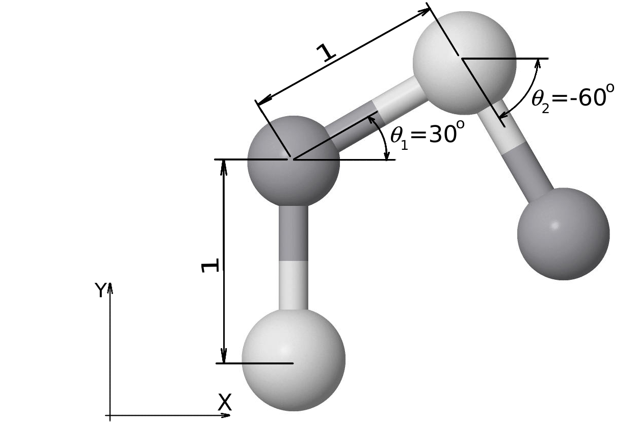
(a)

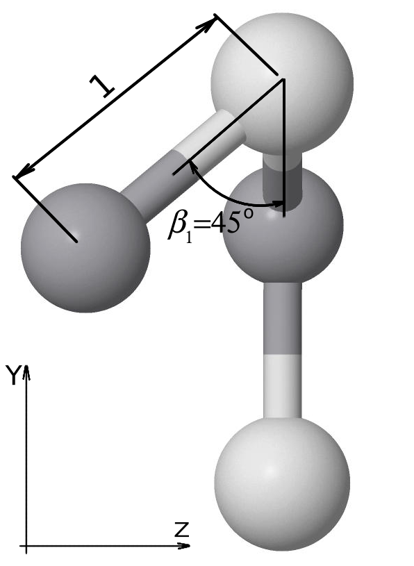
(b)

Figure 1: A schematic diagram of the sequence ABAB. (a) Projection of a structure with $\theta_{1}=30$, $\theta_{2}=-60$ and $\beta_{1}=0$ onto the XY-plane. (b) Projection of a structure with $\theta_{1}=30$, $\theta_{2}=-60$ and $\beta_{1}=45$ onto the ZY-plane.

In our recent work BoskovicAB16 , we proposed a Differential Evolution algorithm that is adapted to PFO on a three-dimensional AB off-lattice model. In contrast to previous population-based algorithms for PFO, this algorithm was designed to follow only one attractor. Within this algorithm, we incorporated a self-adaptive mechanism, a mutation strategy for the fast convergence speed and a temporal locality. The obtained results of this algorithm show that it is superior to the algorithms from the literature, including the artificial bee colony algorithm, and significantly lower free energy values were obtained for longer AB sequences.

3 Three-dimensional AB off-lattice model

The basic building blocks of proteins are amino acids. The linear chain of amino acids is a polypeptide, and a protein contains at least one long polypeptide. Each polypeptide can be represented with a unique amino acid sequence. The polypeptide must fold into a specific three-dimensional native structure before it can perform its biological function(s) petsko2004 . Thus, all information necessary for folding must be contained in the amino acid sequence, and this is known as the Anfinsen-hypothesis buxbaum2007 .

From the amino acid sequence, it is possible to generate different conformations, which is also dependent on the used model. In general, two types of simplified models exist: Off-lattice and lattice. The lattice model maps each position of amino acid to a point on a discrete lattice. In contrast to the lattice model, the off-lattice model allows any position and, as such, is more accurate. The simplified three-dimensional AB off-lattice model was proposed in Stillinger93 . Instead of 20 standard amino acids, this model uses only two different types of amino acids: $A$ – hydrophobic and $B$ – hydrophilic. Thus, an amino acid sequence is represented as a string $\bm{s}=\{s_{1},s_{2},...,s_{L}\}$, $s_{i}\in\{A,B\}$, where $A$ represents a hydrophobic, $B$ a hydrophilic amino acid and $L$ the length of the sequence. The three-dimensional structure of an AB sequence is defined by bond angles $\bm{\theta}=\{\theta_{1},\theta_{2},...,\theta_{L-2}\}$, torsional angles $\bm{\beta}=\{\beta_{1},\beta_{2},...,$ $\beta_{L-3}\}$ and the unit-length chemical bond between two consecutive amino acids (see Fig. 1).

Different energy calculations can be used within different models. Within an AB model, the free energy value is calculated using a simple trigonometric form of backbone bend potentials $E_{1}(\bm{\theta})$ and a species-dependent Lennard-Jones 12,6 form of non-bonded interactions $E_{2}(\bm{s},\bm{\theta},\bm{\beta})$ as shown in the following equation Stillinger93 :

$$E(\bm{s},\bm{\theta},\bm{\beta}) = E_{1}(\bm{\theta})+E_{2}(\bm{s},\bm{\theta},\bm{\beta})$$

$$E_{\text{\tiny 1}}(\bm{\theta}) = \frac{1}{4}\displaystyle\sum_{i=1}^{L-2}[1-cos(\theta_{i})]$$ (1)

$$E_{\text{\tiny 2}}(\bm{s},\bm{\theta},\bm{\beta}) = 4\displaystyle\sum_{i=1}^{L-2}\displaystyle\sum_{\text{{\it j}={\it i}+}2}^{L}[d(\bm{p}_{i},\bm{p}_{j})^{\text{--}12}\text{--}c(s_{i},s_{j})\cdot d(\bm{p}_{i},\bm{p}_{j})^{\text{--}6}]$$

where $\bm{p}_{i}=\{x_{i},y_{i},z_{i}\}$ represents the position of the $i$-th amino acid within the three-dimensional space. These positions are determined as shown in Fig. 1 and by the following equation:

$$\bm{p}_{i}=\begin{cases}\{0,0,0\}&\text{if}~{}i=1,\\ \{0,1,0\}&\text{if}~{}i=2,\\ \{cos(\theta_{1}),1+sin(\theta_{1}),0\}&\text{if}~{}i=3,\\ \{x_{i-1}+cos(\theta_{i-2})\cdot cos(\beta_{i-3}),\\ ~{}~{}y_{i-1}+sin(\theta_{i-2})\cdot cos(\beta_{i-3}),&\text{if 4}\leq i\leq L.\\ ~{}~{}z_{i-1}+sin(\beta_{i-3})\}\\ \end{cases}$$ (2)

In Eq. (3) $d(\bm{p}_{i},\bm{p}_{j})$ denotes the Euclidean distance between positions $\bm{p}_{i}$ and $\bm{p}_{j}$, while $c(s_{i},s_{j})$ determines the attractive, weak attractive or weak repulsive non-bonded interaction for the pair $s_{i}$ and $s_{j}$, as shown in the following equation:

$$c(s_{i},s_{j})=\begin{cases}1&\text{if }s_{i}=A\text{ and }s_{j}=A,\\ 0.5&\text{if }s_{i}=B\text{ and }s_{j}=B,\\ -0.5&\text{if }s_{i}\neq s_{j}.\\ \end{cases}$$

The objective of PFO within the context of an AB off-lattice model is to simulate the folding process and to find the angles’ vector or conformation that minimizes the free-energy value:

$$\{\bm{\theta}^{*},\bm{\beta}^{*}\}=\operatorname*{arg\,min}E(\bm{s},\bm{\theta},\bm{\beta}).$$

4 Method

In this paper, we extend our Differential Evolution algorithm BoskovicAB16 with two new mechanisms. The first mechanism is a local search that improves convergence speed and reduces runtime complexity for solution evaluation within a specific neighborhood. The second mechanism is component reinitialization, which allows the algorithm to locate good similar conformations according to the local best solution.

1: procedure DE${}_{\text{lscr}}$($\bm{s},\mathit{Np}$) 

2:    Initialize a population $P$ $\{\bm{x}_{i},~{}~{}F_{i}=0.5,~{}~{}\mathit{Cr}_{i}=0.9,~{}~{}e_{i}=$$E$($\bm{s},\bm{x_{i}}$)$\}\in P$ $x_{i,j}=-\pi+2\cdot\pi\cdot\mathit{rand}_{[0,1]}$ $i=1,2,...,\mathit{Np};~{}~{}j=1,2,...,D;~{}~{}D=2\cdot$ $length$($\bm{s}$)$-5$$\{\bm{x}_{b},e_{b}\}=\{\bm{x}_{b}^{l},e_{b}^{l}\}=\{\bm{x}_{b}^{p},e_{b}^{p}\}=$ BEST($P$)

3:    while stopping criteria is not met do

4:       for $i=1$ to $\mathit{Np}$ do

5:          if $\mathit{rand}_{[0,1]}<0.1$ then $F=0.1+0.9\cdot\mathit{rand}_{[0,1]}$ else $F=F_{i}$ end if

6:          if $\mathit{rand}_{[0,1]}<0.1$ then $\mathit{Cr}=\mathit{rand}_{[0,1]}$ else $\mathit{Cr}=\mathit{Cr}_{i}$ end if

7:          do $r_{{}_{1}}\text{=}\mathit{rand}_{\{1,\mathit{Np}\}}$ while $r_{{}_{1}}\text{=}i$ end do

8:          do $r_{{}_{2}}\text{=}\mathit{rand}_{\{1,\mathit{Np}\}}$ while $r_{{}_{2}}\text{=}i~{}\text{\bf or}~{}r_{{}_{2}}\text{=}r_{{}_{1}}$ end do

9:          $j_{\mathit{rand}}=\mathit{rand}_{\{1,\mathit{D}\}}$

10:          for $j=1$ to $D$ do

11:             if $\mathit{rand}_{[0,1]}<\mathit{Cr}~{}\text{\bf or }~{}j=j_{\mathit{rand}}$ then

12:                $u_{j}=x_{b,j}+F\cdot(x_{r_{1},j}-x_{r_{2},j})$

13:                if $u_{j}\leq\text{-}\pi$ then $u_{j}\text{\,=\,}2\cdot\pi+u_{j}$ end if

14:                if $u_{j}>\pi$ then $u_{j}\text{\,=\,}2\cdot(\text{-}\pi)+u_{j}$ end if

15:             else

16:                $u_{j}=x_{i,j}$

17:             end if

18:          end for

19:          $e_{u}=$$E$($\bm{s},\bm{u}$) // Energy calculation

20:          if $e_{u}\leq e_{i}$ then

21:             // Temporal locality

22:             for $j=1$ to $D$ do

23:                $u^{*}_{j}=x_{b,j}+0.5\cdot(u_{j}-x_{i,j})$

24:                if $u^{*}_{j}\leq\text{-}\pi$ then $u^{*}_{j}\text{\,=\,}2\cdot\pi+u^{*}_{j}$ end if

25:                if $u^{*}_{j}>\pi$ then $u^{*}_{j}\text{\,=\,}2\cdot(\text{-}\pi)+u^{*}_{j}$ end if

26:             end for

27:             $e^{*}_{u}=$$E$($\bm{s},\bm{u}^{*}$)

28:             if $e^{*}_{u}\leq e_{u}$ then

29:                $\{\bm{x_{i}},F_{i},\mathit{Cr_{i}},e_{i}\}=\{u^{*},F,\mathit{Cr},e^{*}_{u}\}$

30:             else

31:                $\{\bm{x_{i}},F_{i},\mathit{Cr_{i}},e_{i}\}=\{u,F,\mathit{Cr},e_{u}\}$

32:             end if

33:             // Local Search

34:             for $n=2$ to $L-1$ do

35:                $\theta_{n\text{-}1}=\mathit{rand}_{[0,1]}\cdot(x^{p}_{b,n\text{-}1}-x_{i,n\text{-}1})$

36:                $\beta_{n\text{-}2}=\mathit{rand}_{[0,1]}\cdot(x^{p}_{b,n+(L\text{-}4)}-x_{i,n+(L\text{-}4)})$

37:                {${\bm{v},e_{v}}\}=$ LOCAL_MOVEMENT($\bm{x}^{p}_{b},n,\theta_{n\text{-}1},\beta_{n\text{-}2}$)

38:                if $e_{v}\leq e_{b}$ then $\{\bm{x}^{p}_{b},e^{p}_{i}\}=\{\bm{v},e_{v}\}$ end if

39:             end for

40:          end if

41:       end for

42:       $\{\bm{x}_{b}^{p},e_{b}^{p}\}=$ BEST($P$)

43:       if $e_{b}^{p}\leq e_{b}$ then $\{\bm{x}_{b},e_{b}\}=\{\bm{x}_{b}^{p},e_{b}^{p}\}$ end if

44:       REINITIALIZATION($\{\bm{x}_{b}^{p},e_{b}^{p}\}$,$\{\bm{x}_{b}^{l},e_{b}^{l}\}$,$P$)

45:    end while

46:    return  $\{\bm{x}_{b},e_{b}\}$

47: end procedure

Figure 2: The proposed DE${}_{\text{lscr}}$ algorithm.

4.1 Proposed algorithm

Hereinafter, we will describe briefly the DE${}_{\text{lscr}}$ algorithm that is shown in Fig. 2. The lines that represent improvements according to the previous version are highlighted with a gray background. The optimization process begins with initialization (line 2). Each iteration of the $\mathit{while}$ loop (line 3) represents one generation of the evolutionary process. Mutation, crossover, and selection are performed for each population’s individual {$\bm{x}_{1},\bm{x}_{2},...,\bm{x}_{\mathit{Np}}$} within one generation. The $\textit{DE/best/}1$ mutation strategy and binary crossover (lines 7 – 18) are used for creating a trial individual $\bm{u}$. The values of mutation $F$, and crossover $Cr$ control parameters are set with the self-adaptive jDE mechanism (lines 5 and 6) Brest06 . The trial individual is evaluated in line 19 using Eq. (3). From this line, we can see that the individuals are D-dimensional vectors that contain real coded bond $\bm{\theta}$ and torsional $\bm{\beta}$ angles:

$$\bm{x}_{i} = \{x_{i,1},x_{i,2},...,x_{i,D}\}=$$

$$= \{\theta_{1},\theta_{2},...,\theta_{L-2},\beta_{1},\beta_{2},...,\beta_{L-3}\}$$

$$x_{i,j} \in [-\pi,\pi];~{}~{}~{}D=2\cdot L-5$$

$$i = 1,2,...,\mathit{Np};~{}~{}~{}j=1,2,...,D.$$

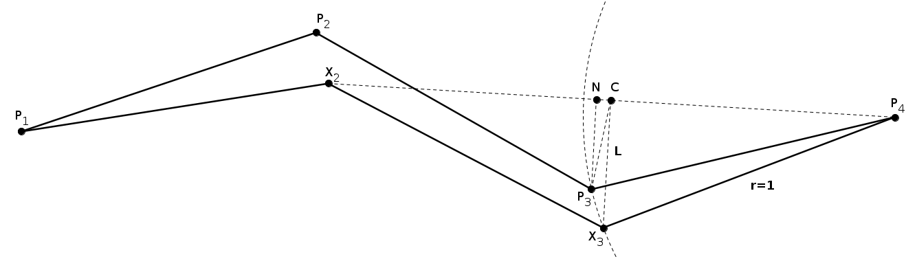
Figure 3: A schematic diagram of a local movement. The polygon $\bm{P_{1}}$, $\bm{P_{2}}$, $\bm{P_{3}}$, $\bm{P_{4}}$ is transformed to polygon $\bm{P_{1}}$, $\bm{X_{2}}$, $\bm{X_{3}}$, $\bm{P_{4}}$ in such a way that only the two consecutive points $\bm{P_{2}}$ and $\bm{P_{3}}$ are moved to points $\bm{X_{2}}$ and $\bm{X_{3}}$, while the remaining points $\bm{P_{1}}$ and $\bm{P_{4}}$ stay unchanged in their positions.

The selection mechanism, temporal locality and local search are shown in lines 20 – 40. If the trial vector is better than the corresponding vector from the population ($e_{u}<e_{i}$), then the second trial vector $\bm{u}^{*}$ is generated using temporal locality Wong12 , and the better vector replaces population vector $\bm{x}_{i}$. The next mechanism is a local search. Within this mechanism, a local movement is used for improving the best population individual $\bm{x}_{b}^{p}$ according to each pair $\{\theta_{n-1},\beta_{n-2}\}$. The values of $\{\theta_{n-1},\beta_{n-2}\}$ represent the angles that specify the position of the ($n+1$)-th monomer according to the position of the $n$-th monomer. After each generation, either random or component reinitialization will be performed if the reinitialization criteria are satisfied (line 44). At the end of the evolutionary process, the algorithm returns the best obtained solution $\bm{x}_{b}$ and its energy value $e_{b}$, as shown in line 46. The local search and reinitialization are described in more detail in the following subsections. For a detailed description of the rest mechanisms that were described briefly within this paragraph, we refer readers to BoskovicAB16 .

4.2 Local search

The temporal locality and local search are performed if the trial vector is better than the corresponding population vector. The local search calculates the values of pair $\{\theta_{n-1},\beta_{n-2}\}$ for each monomer, with the exception of the first two monomers. The positions of these two monomers are fixed within the AB-model, see Eq. (2). For the rest of the monomers, the angle values are defined with a randomly scaled difference between the best population individual $\bm{x}_{b}^{p}$ and current individual $\bm{x}_{i}$, as shown in the following equation:

$$\theta_{n-1} = \mathit{rand}_{[0,1]}\cdot(x^{p}_{b,n-1}-x_{i,n-1})$$

$$\beta_{n-2} = \mathit{rand}_{[0,1]}\cdot(x^{p}_{b,n+(L-4)}-x_{i,n+(L-4)})$$

$$i = 1,...,\mathit{Np};~{}~{}~{}n=2,...,L-1;$$

A meticulous reader may notice that the $\theta$ has index $n-1$, while $\beta$ has index $n-2$. This means that, for $n=2$, the value of $\beta_{0}$ is calculated using the values of $\theta$ components. The reason for that is in the position of the third monomer, which is dependent only on the $\theta_{1}$, see Eq. (2). Therefore, within the local movement for $n=2$, the value of $\beta_{0}$ is ignored, and local movement takes into account only the value of $\theta_{1}$.

The local movement is a transformation of conformation whereby only two consecutive monomers are moved locally in such a way that the remaining mono-mers remain in their positions. There is only one exception, for the last monomer only one monomer is moved, while all the remaining monomers remain in their positions. Fig. 3 shows an example of two monomers’ local movement. The polygon that is defined with points $\bm{P_{1}}$, $\bm{P_{2}}$, $\bm{P_{3}}$, $\bm{P_{4}}$ represents the section of original conformation where points represent the monomer positions. The local movement moves the point $\bm{P_{2}}$ to the point $\bm{X_{2}}$ according to the pair $\{\theta_{n-1},\beta_{n-2}\}$ while the position of point $\bm{X_{3}}$ is calculated using Eqs. (3) – (6). In these calculations, the point $\bm{X_{3}}$ is the nearest to the point $\bm{P_{3}}$ in such a way that the new polygon $\bm{P_{1}}$, $\bm{X_{2}}$, $\bm{X_{3}}$, $\bm{P_{4}}$ must end at the point $\bm{P_{4}}$.

The calculation begins with the determination of point $\bm{C}$, whose position is in the middle of points $\bm{P_{4}}$ and $\bm{X_{2}}$:

$$\bm{C}=\bm{X_{2}}+\frac{\bm{P_{4}}-\bm{X_{2}}}{2}.$$ (3)

The length $L$ between points $\bm{C}$ and $\bm{X_{3}}$ is calculated by using the triangle $\bm{P_{4}}$, $\bm{C}$, $\bm{X_{3}}$ and Pythagoras’s theorem:

$$L=\sqrt{1-\frac{\left\lVert\bm{P_{4}}-\bm{X_{2}}\right\rVert^{2}}{4}}.$$ (4)

The vector projection of $(\bm{P_{3}}-\bm{C})$ onto line $\bm{X_{2}}$, $\bm{P_{4}}$ is calculated with the following equation:

$$\bm{C_{N}}=(\bm{P_{3}}-\bm{C})\cdot\frac{\bm{P_{4}}-\bm{X_{2}}}{\left\lVert\bm{P_{4}}-\bm{X_{2}}\right\rVert}.$$ (5)

At the end, point $\bm{X_{3}}$ is calculated by scaling of vector $(\bm{P_{3}}-\bm{C})-\bm{C_{N}}$ as follows:

$$\bm{X_{3}}=\bm{C}+\frac{(\bm{P_{3}}-\bm{C})-\bm{C_{N}}}{\left\lVert(\bm{P_{3}}-\bm{C})-\bm{C_{N}}\right\rVert}\cdot L.$$ (6)

The created polygon contains unchanged points $\bm{P_{1}}$ and $\bm{P_{4}}$, which means only monomers $\bm{X_{2}}$ and $\bm{X_{3}}$ are moved locally, while the remaining monomers stay in their unchanged positions. This feature allows us to design the fast conformation evaluation within the local movement. Two additional data structures, $\bm{E_{1}}$ and $\bm{E_{2}}$, were used for this purpose. The values of elements within these data structures are determined according to Eq. (3), as follows:

$$\mathit{E}_{1_{i}} = 1-cos(\theta_{i})$$

$$\mathit{E}_{2_{i,j}} = d(\bm{p}_{i},\bm{p}_{j})^{-12}-c(s_{i},s_{j})\cdot d(\bm{p}_{i},\bm{p}_{j})^{-6}$$

$$i \in \{1,...,L-2\};~{}~{}~{}j\in\{i+2,...,L\}.$$

Using these data structures for the best population individual and its energy value, we can calculate the energy of the conformation created by local movement efficiently, as is shown in Eqs. (4.2) – (9), where $n$ represents the variable that was sent to the local movement procedure, as shown in Fig. 2 (see line 37).

$$\Delta e_{1} = \mathit{E}_{1_{n-1}}-(1-cos(\theta_{n-1}))+$$

$$\mathit{E}_{1_{n}}-(1-cos(\theta_{n}))+$$

$$\mathit{E}_{1_{n+1}}-(1-cos(\theta_{n+1}))$$

$$\Delta e_{2} = \sum_{i=n+1}^{n+3}\sum_{j=n+2}^{L}\Big{[}\mathit{E}_{2_{i,j}}-$$

$$\big{(}d(\bm{p}_{i},\bm{p}_{j})^{-12}-c(s_{i},s_{j})\cdot d(\bm{p}_{i},\bm{p}_{j})^{-6}\big{)}\Big{]}+$$ (8)

$$\sum_{i=n+1}^{n+3}\sum_{j=1}^{i}\Big{[}\mathit{E}_{2_{j,i}}-$$

$$\big{(}d(\bm{p}_{i},\bm{p}_{j})^{-12}-c(s_{i},s_{j})\cdot d(\bm{p}_{i},\bm{p}_{j})^{-6}\big{)}\Big{]}$$

$$e_{v}=e^{p}_{b}-(\frac{\Delta e_{1}}{4}+4\cdot\Delta e_{2})$$ (9)

From Eqs. (4.2) – (9) we can observe that the time complexity of energy calculation is reduced from $\frac{L^{2}}{2}$ to $2L$. In this way, the designed local movement allows faster evaluation of neighborhood solutions, and its usage within local search improves convergence speed.

4.3 Reinitialization

After each generation, reinitialization will be performed if the reinitialization criteria are satisfied. In our previous work, random reinitialization was performed if the best population individual stayed unchanged within the evolution process for more than $10^{5}$ evaluations. This number includes the number of evaluations for all individuals until the best population individual stayed unchanged. Its value was determined in a way to prevent premature restarts, and to ensure some likelihood that the algorithm cannot improve the best population individual by using the current population. In this work, we design a new reinitialization mechanism which has some advantages over our previous work. For that purpose, the algorithm includes three types of the best individuals and three new control parameters, as shown in Fig. 4. The individuals $\bm{x}^{p}_{b},\bm{x}^{l}_{b},\bm{x}_{b}$ represent the best population, local best and global best individuals. The best population individual is the best individual in the current population, the local best individual is the best individual among all similar individuals, and the global best individual is the best individual obtained within the evolutionary process. From this description of the best individuals, we can see that the main advantages of the proposed reinitialization are to allow the following:

1: procedure REINITIALIZATION($\{\bm{x}_{b}^{p},e_{b}^{p}\}$,$\{\bm{x}_{b}^{l},e_{b}^{l}\}$,$P$) 

2:    if $\bm{x}_{b}^{p}$ is unchanged for at least $P_{b}\cdot D$ evaluations then

3:       if $e_{b}^{p}\leq e_{b}^{l}$ then $\{\bm{x}_{b}^{l},e_{b}^{l}\}=\{\bm{x}_{b}^{p},e_{b}^{p}\}$ end if

4:       if $\bm{x}_{b}^{l}$ is unchanged for $L_{b}\cdot D$ reinitializations then

5:          // Random reinitialization

6:          $\bm{x}_{i}=$ RANDOM() ;    $i=1,2,...,\mathit{Np}$

7:          $\{\bm{x}_{b}^{l},e_{b}^{l}\}=\{\bm{x}_{b}^{p},e_{b}^{p}\}=$ BEST($P$)

8:       else

9:          // Component reinitialization

10:          $\bm{x}_{i}=$ RANDOM($\bm{x}_{b}^{l},C$);    $i=1,2,...,\mathit{Np}$

11:          $\{\bm{x}_{b}^{p},e_{b}^{p}\}=$ BEST($P$)

12:       end if

13:    end if

14: end procedure

Figure 4: The reinitialization mechanism.

• Locate the best individual by using the current population,

• Locate the best similar individual by using component reinitialization, and

• Locate the global best individual by using random reinitialization.

Table 1: Details of amino acid sequences used in experiments.

Label	Length	$D$	Sequence
1BXP	13	21	ABBBBBBABBBAB
1CB3	13	21	BABBBAABBAAAB
1BXL	16	27	ABAABBAAAAABBABB
1EDP	17	29	ABABBAABBBAABBABA
2ZNF	18	31	ABABBAABBABAABBABA
1EDN	21	37	ABABBAABBBAABBABABAAB
2H3S	25	45	AABBAABBBBBABBBABAABBBBBB
1ARE	29	53	BBBAABAABBABABBBAABBBBBBBBBBB
2KGU	34	63	ABAABBAABABBABAABAABABABABABAAABBB
1TZ4	37	69	BABBABBAABBAAABBAABBAABABBBABAABBBBBB
1TZ5	37	69	AAABAABAABBABABBAABBBBAABBBABAABBABBB
1AGT	38	71	AAAABABABABABAABAABBAAABBABAABBBABABAB
1CRN	46	87	BBAAABAAABBBBBAABAAABABAAAABBBAAAAAAAABAAABBAB
2KAP	60	115	BBAABBABABABABBABABBBBABAABABAABBBBBBABBBAABAAABBABBABBAAAAB
1HVV	75	145	BAABBABBBBBBAABABBBABBABBABABAAAAABBBABAABBABBBABBAABBABBAABBBB
			BAABBBBBABBB
1GK4	84	163	ABABAABABBBBABBBABBABBBBAABAABBBBBAABABBBABBABBBAABBABBBBBAABAB
			AAABABAABBBBAABABBBBA
1PCH	88	171	ABBBAAABBBAAABABAABAAABBABBBBBABAAABBBBABABBAABAAAAAABBABBABABA
			BABBABBAABAABBBAABBAAABA
2EWH	98	191	AABABAAAAAAABBBAAAAAABAABAABBAABABAAABBBAAAABABAAABABBAAABAAABA
			AABAABBAABAAAAABAAABABBBABBAAABAABA
F13	13	21	ABBABBABABBAB
F21	21	37	BABABBABABBABBABABBAB
F34	34	63	ABBABBABABBABBABABBABABBABBABABBAB
F55	55	105	BABABBABABBABBABABBABABBABBABABBABBABABBABABBABBABABBAB
F89	89	173	ABBABBABABBABBABABBABABBABBABABBABBABABBABABBABBABABBABABBABBAB
			ABBABBABABBABABBABBABABBAB

The following new control parameters are introduced to the reinitialization mechanism: $P_{b},L_{b}$, and $C$. In our previous work, the reinitialization was defined with a constant number of evaluations ($10^{5}$). In this work, restarts are dependent on the values of parameters $P_{b}$, $L_{b}$ and the dimension of the problem. The $P_{b}$ defines how long the best population individual can stay unchanged within the evolutionary process (line 2). For example, with $P_{b}=100$ and dimension $21$, the reinitialization is performed if the best population individual would stay unchanged in the evolutionary process for at least $P_{b}\cdot D=100\cdot 21=2100$ evaluations. When this condition is satisfied, the algorithm performs random or component reinitialization according to the parameter $L_{b}$. If the local best individual is not changed for $L_{b}\cdot D$ reinitializations, then random reinitialization is performed, and component reinitialization otherwise (line 4). The last parameter $C$ determines the number of components that are different between the local best individual and individuals generated by component reinitialization (line 10). Within the component reinitialization, the $C$ components of each population individual $\bm{x}_{i}$ are selected randomly, and their values are replaced with random values on the interval $[-\pi,\pi]$, while all the remaining components get the values from the local best individual.

5 Experiments

The DE${}_{\text{lscr}}$ algorithm was compiled with a GNU C++ compiler 4.6.3 and executed using an Intel Core i7 computer with 2.93 GHz CPU and 8 GB RAM under Linux Mint 13 Maya and a grid environment (Slovenian Initiative for National Grid). In order to evaluate the efficiency of the proposed algorithm, we used a set of amino acid sequences as shown in Table 1. This set includes 5 Fibonacci sequences and 18 real peptide sequences from the Protein Data Bank database. The K-D method is used to transform real peptide sequences to the AB sequences. In this method, the amino acids I, V, P, L, C, M, A, and G are transformed to hydrophobic ones (A) and amino acids D, E, H, F, K, N, Q, R, S, T, W, and Y to hydrophilic ones (B). The selected sequences have different lengths, which enabled us to analyze the algorithm according to different problem dimensions and, because they were used frequently in literature, they enabled us to compare the proposed algorithm with different algorithms. In order to analyze the efficiency of the introduced mechanisms and algorithm, we measured the following statistics:

• The mean obtained energy value for all runs:

  $$E_{\mathit{mean}}=\frac{\sum_{i=1}^{N}E_{i}}{N}$$

  where $E_{i}$ denotes the obtained energy value for the $i$-th run and $N$ is the number of runs.

• The best obtained energy value among all runs:

  $$E_{\mathit{best}}=max\{E_{1},E_{2},...,E_{N}\}.$$

  Note that all energy values within our experiments are multiplied by $-1$, which means that all energy values are positive and higher values are better.

• The standard deviation of energy values for all runs:

  $$E_{\mathit{std}}=\sqrt{\frac{\sum_{i=1}^{N}{(E_{i}-E_{\mathit{mean}})}^{2}}{N-1}}$$

• The hit ratio or percentage of runs during which the best solution has equal or better energy value according to the target value ($target$):

  $$\mathit{hit_{r}}=\frac{N_{h}}{N}$$

  where $N_{h}$ denotes the number of runs where the best obtained solution has good enough energy value $e_{b}$ according to the target value ($e_{b}\geq\mathit{target}$).

• The mean number of solution evaluation for all $N_{h}$ runs:

  $$\mathit{NSE}_{\mathit{mean}}=\frac{\sum_{i=1}^{N_{h}}\mathit{NSE}_{i}}{N_{h}}$$

  where $\mathit{NSE}_{i}$ represents the number of solution evaluations for the $i$-th run.

• The standard deviation of solution evaluations for all $N_{h}$ runs:

  $$\mathit{NSE}_{\mathit{std}}=\sqrt{\frac{\sum_{i=1}^{N_{h}}{(\mathit{NSE}_{i}-\mathit{NSE}_{\mathit{mean}})}^{2}}{N_{h}-1}}$$

• The mean runtime for all runs:

  $$\mathit{t}_{mean}=\frac{\sum_{i=1}^{N}\mathit{t_{i}}}{N}$$

  where $\mathit{t_{i}}$ represents the runtime of the $i$-th run.

• The mean speed for all runs:

  $$\mathit{v}_{mean}=\frac{\sum_{i=1}^{N}\mathit{v_{i}}}{N}$$

  where $\mathit{v_{i}}$ represents the speed (the number of solution evaluations per second) of the $i$-th run.

The listed statistics were measured within the context of the following stopping conditions:

• The maximum number of solution evaluations
  $\mathit{NSE_{\mathit{lmt}}}$: $\mathit{NSE}_{i}\geq\mathit{NSE}_{lmt}$.

• The runtime limit $\mathit{t_{lmt}}$: $t_{i}\geq t_{lmt}$.

• The energy value of the best obtained solution
  $\mathit{target}$: $e_{b}\geq\mathit{target}$.

Our algorithm belongs to stochastic algorithms, therefore, all the reported results of the proposed algorithm within this work are based on $N=100$ independent runs. The described statistics, the defined stopping criteria and the determined number of independent runs were used to analyze the influence of new parameters and mechanisms on the algorithm’s efficiency. The algorithm was also compared with the state-of-the art algorithms. The asymptotic average-case performances were determined for the 6 shortest sequences, and an analysis of the obtained conformations was also performed and will be given in the continuation of the paper.

Table 2: The analysis of the new control parameters ($P_{b},L_{b},C$). $N=100$ independent runs were performed for each setting and the stopping conditions were the maximum number of solution evaluations $\mathit{NSE_{\mathit{lmt}}}=10^{10}$ and target value.

$P_{b}$	$L_{b}$	$C$	$E_{\mathit{mean}}$	$E_{\mathit{std}}$	$\mathit{hit_{r}}$	$\mathit{NSE}_{\mathit{mean}}$	$\mathit{NSE}_{\mathit{std}}$
50	2	5	6.9961	0.00	100	6.41E+07	5.59E+07
100	2	5	6.9961	0.00	100	6.88E+07	5.96E+07
25	2	5	6.9961	0.00	100	7.52E+07	7.01E+07
50	5	5	6.9961	0.00	100	9.07E+07	8.06E+07
50	2	10	6.9961	0.00	100	9.52E+07	9.67E+07
50	1	5	6.9961	0.00	100	9.59E+07	9.55E+07
50	10	5	6.9961	0.00	100	9.77E+07	9.48E+07
50	2	2	6.9847	0.03	90	3.15E+09	2.67E+09

(a) F13, $target=6.9961$

$P_{b}$	$L_{b}$	$C$	$E_{\mathit{mean}}$	$E_{\mathit{std}}$	$\mathit{hit_{r}}$	$\mathit{NSE}_{\mathit{mean}}$	$\mathit{NSE}_{\mathit{std}}$
25	20	5	16.4500	0.09	21	4.91E+09	2.75E+09
25	10	5	16.4492	0.08	19	4.89E+09	2.81E+09
50	10	5	16.4432	0.08	17	3.92E+09	2.98E+09
50	20	5	16.4415	0.10	22	4.86E+09	3.17E+09
10	20	5	16.4307	0.09	15	3.93E+09	2.51E+09
25	50	5	16.4254	0.12	33	4.84E+09	2.85E+09
25	20	10	16.4037	0.08	2	7.94E+09	2.53E+09
25	20	2	15.4393	0.45	0	-	-

(b) F21, $target=16.5544$

$P_{b}$	$L_{b}$	$C$	$E_{\mathit{mean}}$	$E_{\mathit{std}}$
50	10	5	30.0670	0.45
50	20	5	30.0596	0.40
25	10	5	30.0519	0.47
50	5	5	29.9108	0.38
100	10	5	29.9034	0.47
50	10	10	29.3722	0.35
50	10	2	24.2650	1.94

(c) F34

$P_{b}$	$L_{b}$	$C$	$E_{\mathit{mean}}$	$E_{\mathit{std}}$
25	5	10	49.0262	0.78
25	10	10	49.0233	1.26
10	5	10	49.0148	1.05
50	5	10	48.9379	1.19
25	2	10	48.9192	1.03
25	5	5	47.8458	1.74
25	5	20	47.4250	0.88

(d) F55

$P_{b}$	$L_{b}$	$C$	$E_{\mathit{mean}}$	$E_{\mathit{std}}$
50	2	10	76.8608	1.64
25	2	10	76.6879	1.89
50	5	10	76.5090	1.88
25	5	10	76.4541	1.93
50	1	10	76.3478	1.40
100	2	10	76.3275	1.71
50	2	5	75.1975	2.62
50	2	20	75.0143	1.52

(e) F89

5.1 Parameter settings

The influence of the new control parameters ($P_{b},L_{b},C$) on the algorithm’s efficiency was analyzed by using Fibonacci sequences. In this analysis, the stopping condition was the maximum number of solution evaluations $\mathit{NSE_{\mathit{lmt}}}=10^{10}$. For each sequence, we started with the following setting: $P_{b}=50$, $L_{b}=10$, and $C=5$. Using 6 settings, where only one value of each setting was changed to the nearest higher or lower value, we tried to get better settings. The parameter values are used from the following sets:

$$P_{b} \in \{10,25,50,100\}$$

$$L_{b} \in \{1,2,5,10,20,50\}$$

$$C \in \{2,5,10,20\}$$

For the started setting the following 6 settings were used:

$$\{ \bm{P_{b}=10},L_{b}=10,C=5\},\{\bm{P_{b}=25},L_{b}=10,C=5\},$$

$$\{ P_{b}=50,\bm{L_{b}=5},C=5\},\{P_{b}=50,\bm{L_{b}=20},C=5\},$$

$$\{ P_{b}=50,L_{b}=10,\bm{C=2}\},\{P_{b}=50,L_{b}=10,\bm{C=10}\}.$$

We repeated this process until a new better setting was found. The results of the least iterations, together with recommended settings, are shown in Table 2. For clarity, the recommended settings and their results are shown in bold typeface. The displayed results show that each sequence has its own optimal setting, but it is still possible to select settings that can be used for any unknown sequence. We define these settings according to the dimension of the problem, as follows:

$$\{P_{b},L_{b},C\}=\begin{cases}\{50,10,5\}&\text{if }n<45\\ \{25,5,10\}&\text{otherwise}.\\ \end{cases}$$

These settings are used in all the following experiments, because they can provide a good hit ratio for short sequences and good energy values for longer sequences. The search space for longer sequences is huge, which means the algorithm almost surely cannot reach optimal solutions in a reasonable runtime e.g. 4 days. Therefore, for these sequences, the algorithm has to perform more reinitializations, and the component reinitialization has to change more components randomly.

The displayed results confirm, additionally, that the variable $\mathit{NSE}$ have near-exponential or near-geometric distribution ($\mathit{NSE}_{\mathit{mean}}\approx\mathit{NSE}_{\mathit{std}}$). Under such distributions, given the $N_{h}=100$ runs in all of our experiments, a reliable rule-of-thumb estimates a 95% confidence interval:

$$\mathit{CI}_{95} \approx [(1-\frac{1.96}{\sqrt{N_{h}}})\cdot\mathit{NSE}_{\mathit{mean}},(1+\frac{1.96}{\sqrt{N_{h}}})\cdot\mathit{NSE}_{\mathit{mean}}]$$

$$\approx [0.8\cdot\mathit{NSE}_{\mathit{mean}},1.2\cdot\mathit{NSE}_{\mathit{mean}}].$$

5.2 Local search

Table 3: The influence of the local search to the algorithm’s efficiency according to two algorithms: DE${}_{\text{lscr}}$ - with local search and DE${}_{\text{cr}}$ - without local search. Two different comparisons were made according to two different stopping conditions: $\mathit{NSE}_{\mathit{lmt}}=10^{7}$ and $t_{\mathit{lmt}}=t_{\mathit{mean}}($DE${}_{\text{cr}}$$)$. The reported mean speed $v_{\mathit{mean}}$ represents the mean number of function evaluations per second, $c_{v}$ represents the speed up factor $v_{\mathit{mean}}$(DE${}_{\text{lscr}}$)$/v_{\mathit{mean}}$(DE${}_{\text{cr}}$) and the mean runtime $t_{\mathit{mean}}$ is given in seconds.

Label	$\mathit{NSE}_{\mathit{lmt}}=10^{7}$								$t_{\mathit{lmt}}=t_{\mathit{mean}}($DE${}_{\text{cr}}$$)$
	DE${}_{\text{lscr}}$				DE${}_{\text{cr}}$				DE${}_{\text{lscr}}$
	$t_{\mathit{mean}}$	$v_{\mathit{mean}}$	$E_{\mathit{mean}}$	$E_{\mathit{std}}$	$t_{\mathit{mean}}$	$v_{\mathit{mean}}$	$E_{\mathit{mean}}$	$E_{\mathit{std}}$	$t_{\mathit{mean}}$	$v_{\mathit{mean}}$	$c_{v}$	$E_{\mathit{mean}}$	$E_{\mathit{std}}$
1BXP	12.54	7.98E+05	4.7280	0.24	18.35	5.45E+05	4.6772	0.26	18.35	7.98E+05	1.46	4.7831	0.26
1CB3	12.18	8.22E+05	7.9643	1.02	18.00	5.56E+05	8.1511	0.65	18.00	8.22E+05	1.48	8.1340	0.92
1BXL	15.02	6.67E+05	16.2149	0.51	24.81	4.03E+05	16.2338	0.66	24.81	6.72E+05	1.66	16.3452	0.48
1EDP	16.00	6.25E+05	13.7281	1.07	27.39	3.65E+05	13.3930	1.80	27.39	6.07E+05	1.66	14.1388	0.54
2ZNF	17.44	5.74E+05	16.1670	1.86	29.78	3.36E+05	14.4350	3.01	29.78	5.73E+05	1.70	16.7171	1.24
1EDN	20.27	4.94E+05	17.9565	2.51	38.05	2.63E+05	16.5951	3.10	38.05	4.97E+05	1.89	18.9328	1.85
2H3S	24.85	4.03E+05	15.1685	2.36	50.64	1.98E+05	15.1545	2.79	50.64	4.06E+05	2.06	16.1873	2.34
1ARE	29.37	3.41E+05	19.3024	1.92	63.85	1.57E+05	18.6434	2.48	63.85	3.44E+05	2.20	20.2815	1.80
2KGU	34.89	2.87E+05	43.6622	3.46	84.42	1.19E+05	40.6789	4.66	84.42	2.92E+05	2.46	46.1607	2.28
1TZ4	37.47	2.68E+05	28.7054	4.77	95.07	1.05E+05	25.3528	5.30	95.07	2.74E+05	2.61	31.7309	4.26
1TZ5	36.66	2.73E+05	34.3793	4.36	95.11	1.05E+05	32.9423	5.08	95.11	2.81E+05	2.67	36.7141	4.66
1AGT	38.81	2.58E+05	52.9353	4.99	100.39	9.97E+04	47.6395	5.86	100.39	2.66E+05	2.67	56.5688	3.80
1CRN	51.66	1.94E+05	78.8070	4.74	139.22	7.19E+04	78.8601	5.69	139.22	2.02E+05	2.82	82.8484	2.14
2KAP	76.79	1.31E+05	54.6804	6.60	220.23	4.54E+04	55.3668	6.08	220.23	1.37E+05	3.01	59.9772	5.93
1HVV	104.64	9.62E+04	57.5815	6.55	320.20	3.12E+04	57.3717	6.56	320.20	1.03E+05	3.29	63.5027	6.29
1GK4	122.54	8.23E+04	72.3524	7.15	394.79	2.53E+04	72.8575	7.87	394.79	9.10E+04	3.59	78.8594	6.17
1PCH	130.19	7.76E+04	103.4913	13.35	438.63	2.28E+04	101.7607	11.42	438.63	8.71E+04	3.82	116.0248	11.99
2EWH	162.03	6.24E+04	189.5316	14.33	546.97	1.83E+04	182.2880	16.48	546.97	7.14E+04	3.91	205.3507	10.62
F13	12.42	8.05E+05	6.0591	0.94	18.08	5.53E+05	6.0951	1.09	18.08	8.07E+05	1.46	6.3373	0.83
F21	20.90	4.79E+05	12.0495	1.66	37.84	2.64E+05	11.3298	1.75	37.84	4.82E+05	1.82	12.8967	1.70
F34	35.89	2.79E+05	20.0652	2.59	82.90	1.21E+05	18.3942	2.29	82.90	2.87E+05	2.38	21.4521	2.62
F55	71.27	1.41E+05	35.2611	3.55	191.88	5.21E+04	35.3539	3.02	191.88	1.46E+05	2.80	37.9751	2.44
F89	140.58	7.19E+04	55.4025	5.06	455.38	2.20E+04	55.0803	5.55	455.38	7.92E+04	3.61	59.1793	4.40

Table 4: The influence of the component reinitialization to the algorithm’s efficiency according to two algorithms: DE${}_{\text{lscr}}$ - with component reinitialization and DE${}_{\text{ls}}$ - without component reinitialization. Two stopping conditions were used: $\mathit{NSE}_{\mathit{lmt}}=10^{11}$ and $target$ values that were set to the best-known energy values (see Table 8). The shown $C_{\mathit{NSE}}$ represents the reduction of $\mathit{NSE}_{\mathit{mean}}$: $\mathit{NSE}_{\mathit{mean}}$(DE${}_{\text{lscr}}$) $/$ $\mathit{NSE}_{\mathit{mean}}$(DE${}_{\text{ls}}$).

Label	Length	$D$	$target$	DE${}_{\text{lscr}}$				DE${}_{\text{ls}}$
				$\mathit{NSE}_{\mathit{mean}}$	$C_{\mathit{NSE}}$	$\mathit{NSE}_{\mathit{std}}$	$hit_{r}$	$\mathit{NSE}_{\mathit{mean}}$	$\mathit{NSE}_{\mathit{std}}$	$hit_{r}$
1BXP	13	21	5.6104	1.56E+09	0.38	1.68E+09	100	4.07E+09	4.20E+09	100
1CB3	13	21	8.4589	3.61E+07	0.18	4.26E+07	100	1.99E+08	1.77E+08	100
1BXL	16	27	17.3962	1.24E+10	$<0.37$	1.24E+10	100	3.36E+10	2.71E+10	32
1EDP	17	29	15.0092	4.58E+09	$<0.22$	4.21E+09	100	2.14E+10	2.10E+10	96
2ZNF	18	31	18.3402	2.10E+09	$<0.05$	1.92E+09	100	4.31E+10	2.75E+10	50
F13	13	21	6.9961	8.92E+07	0.08	8.52E+07	100	1.14E+09	1.27E+09	100

The local search within our algorithm was designed to increase the speed of algorithm convergence and speed of neighborhood solution evaluations. In order to demonstrate these advantages, the algorithm was analyzed with (DE${}_{\text{lscr}}$) and without (DE${}_{\text{cr}}$) local search. Within this analysis, the algorithms were compared using the following stopping conditions: $\mathit{NSE}_{\mathit{lmt}}=10^{7}$ and $t_{\mathit{lmt}}=t_{\mathit{mean}}$(DE${}_{\text{cr}}$), as shown in Table 3. With the first stopping condition, we show that the local search improves mean energy value $E_{\mathit{mean}}$ on 16 out of 23 sequences and reduces the mean runtime $t_{\mathit{mean}}$ for all sequences. For the longest sequence 2EWH, $E_{\mathit{mean}}$ was improved from 182.2880 to 189.5316, or by 7.2436, and for this improvement, the runtime was reduced from 546.97 to 162.03 seconds, or by factor 3.376. Using the second stopping condition, both algorithms were limited with the same runtime and, in this case, local search improved $E_{\mathit{mean}}$ in 22 out of 23 sequences. These values are marked in bold typeface within the table. The value 205.3507 was shown in bold typeface for the sequence 2EWH. This means that, by using the local search and $t_{\mathit{lmt}}=546.97$ seconds, $E_{\mathit{mean}}$ was improved by 23.0627. Results also show that the speed up factor $c_{v}$ was 1.46 for the shortest sequences (F13 and 1BXP) and 3.91 for the longest sequence 2EWH, while the $E_{\mathit{mean}}$ is worse by 0.0171 for sequence 1CB3 and better for all other sequences.

From the obtained results, we can conclude that the local search improves the convergence speed of the algorithm for most of the sequences, while the speed of solution evaluation is increased for all sequences. Somebody would expect better speed up factors, but note that some conditions must be satisfied for local search and, therefore, the speed up factor is dependent on the relationship between the number of solution evaluations inside and outside the local search. However, using the local search, the algorithm is capable of obtaining better energy values for almost all sequences, and this improvement of energy values increases for longer sequences.

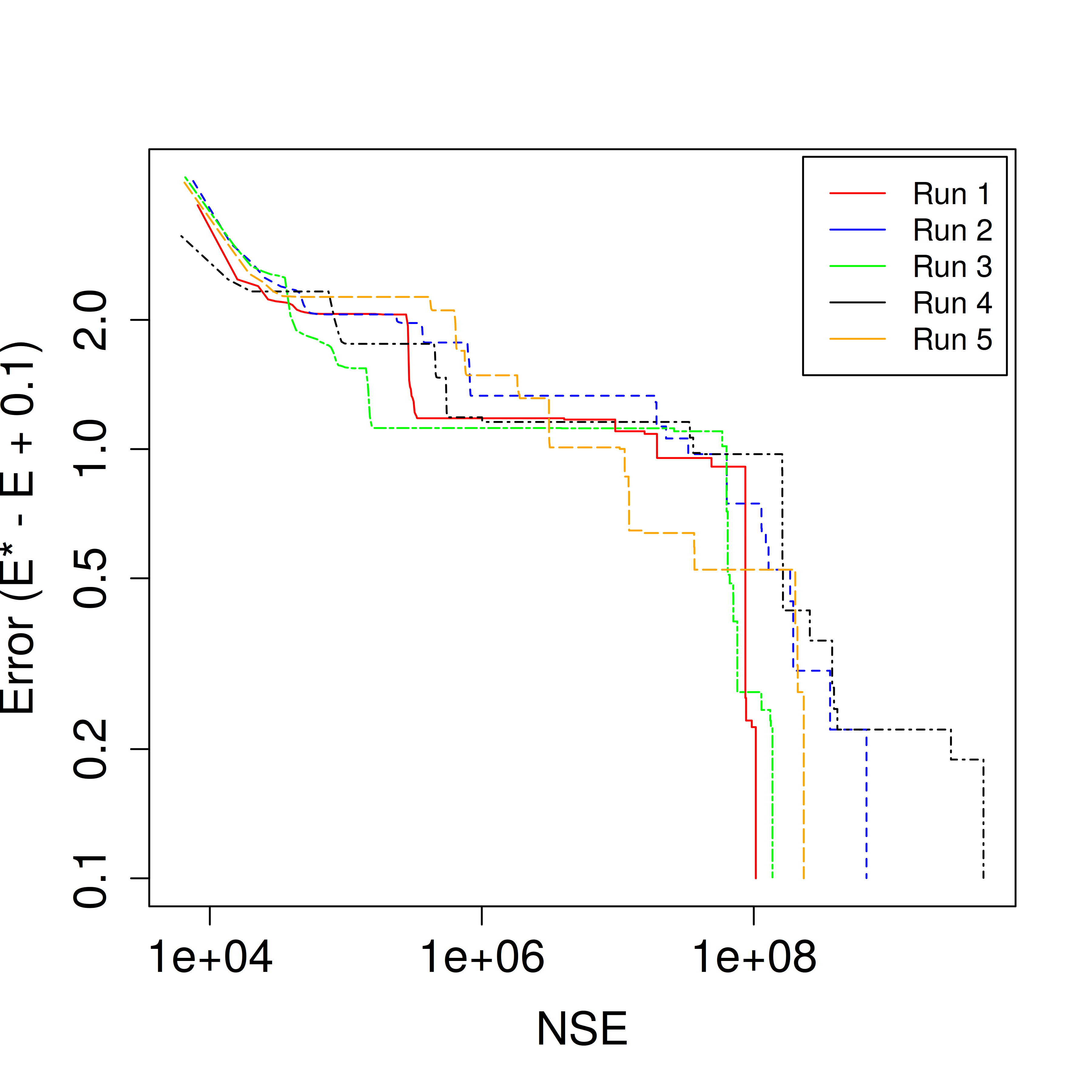
(a) 1BXP

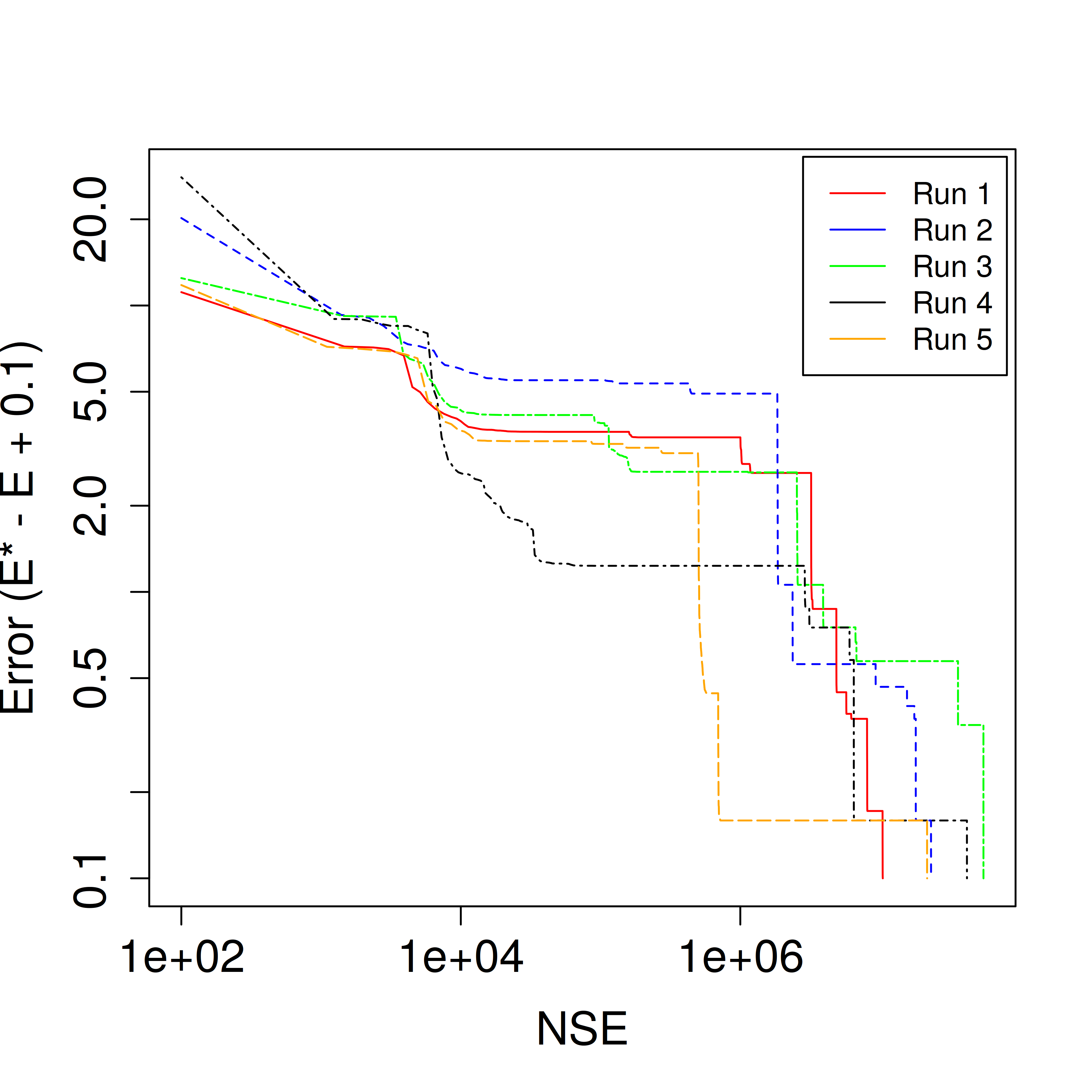
(b) 1CB3

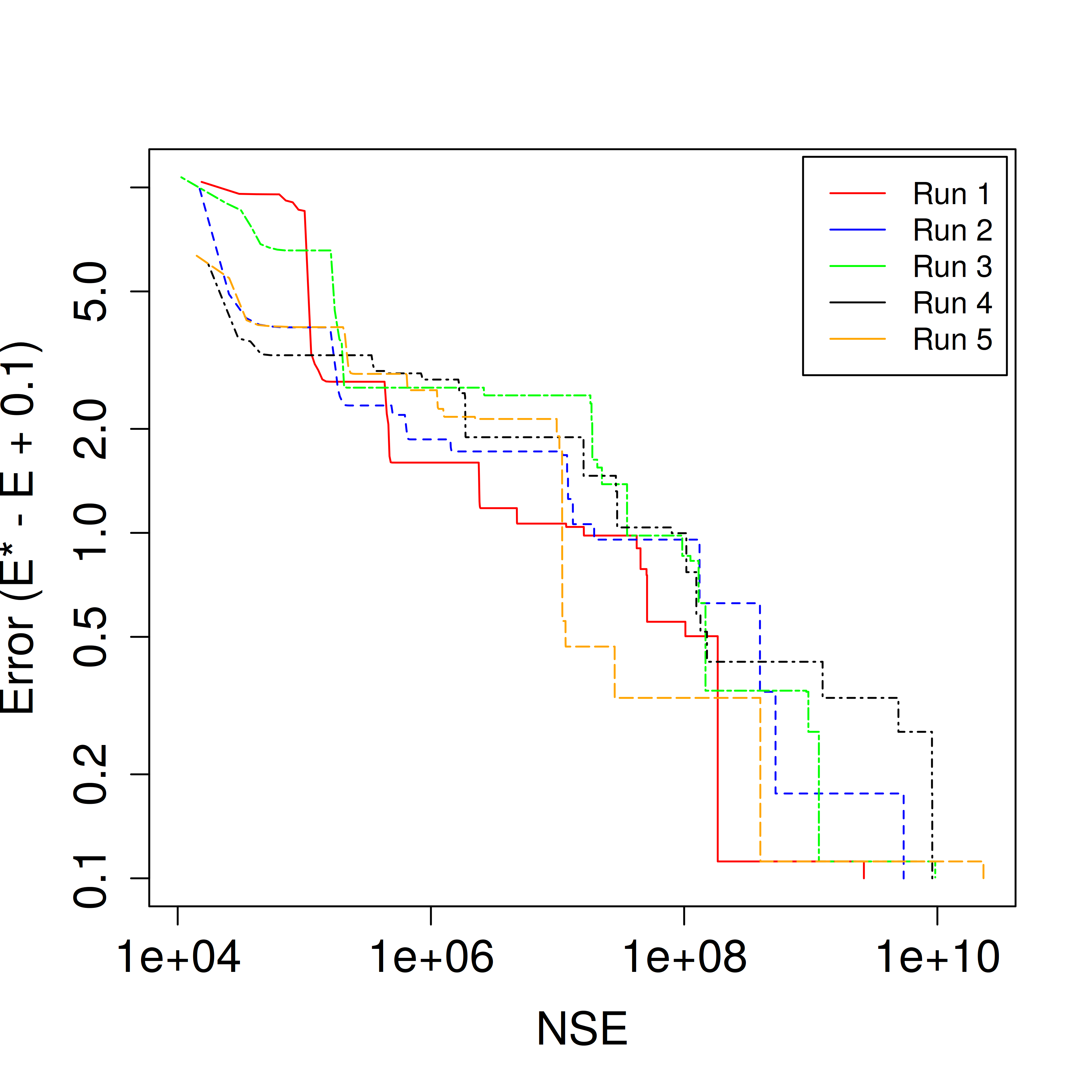
(c) 1BXL

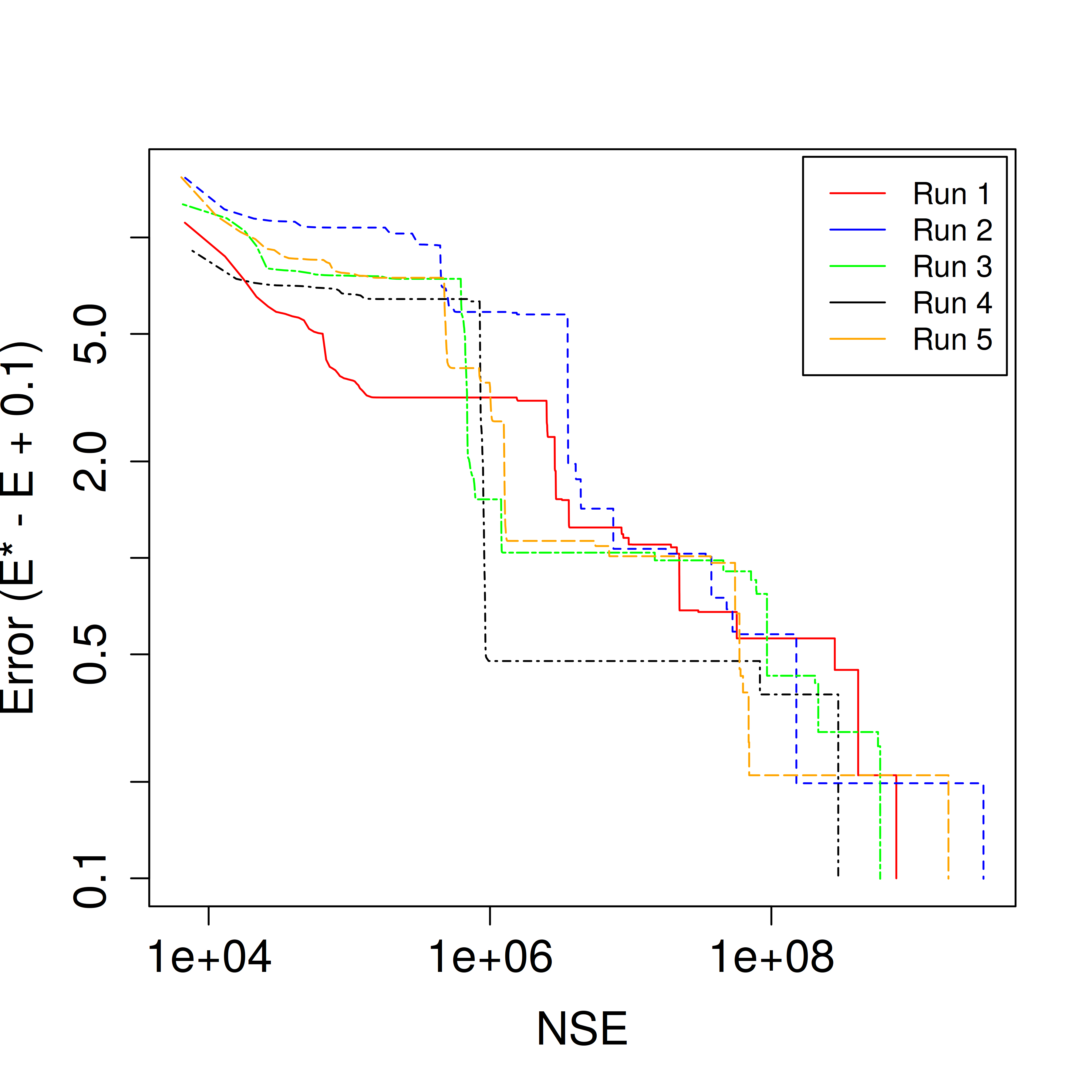
(d) 1EDP

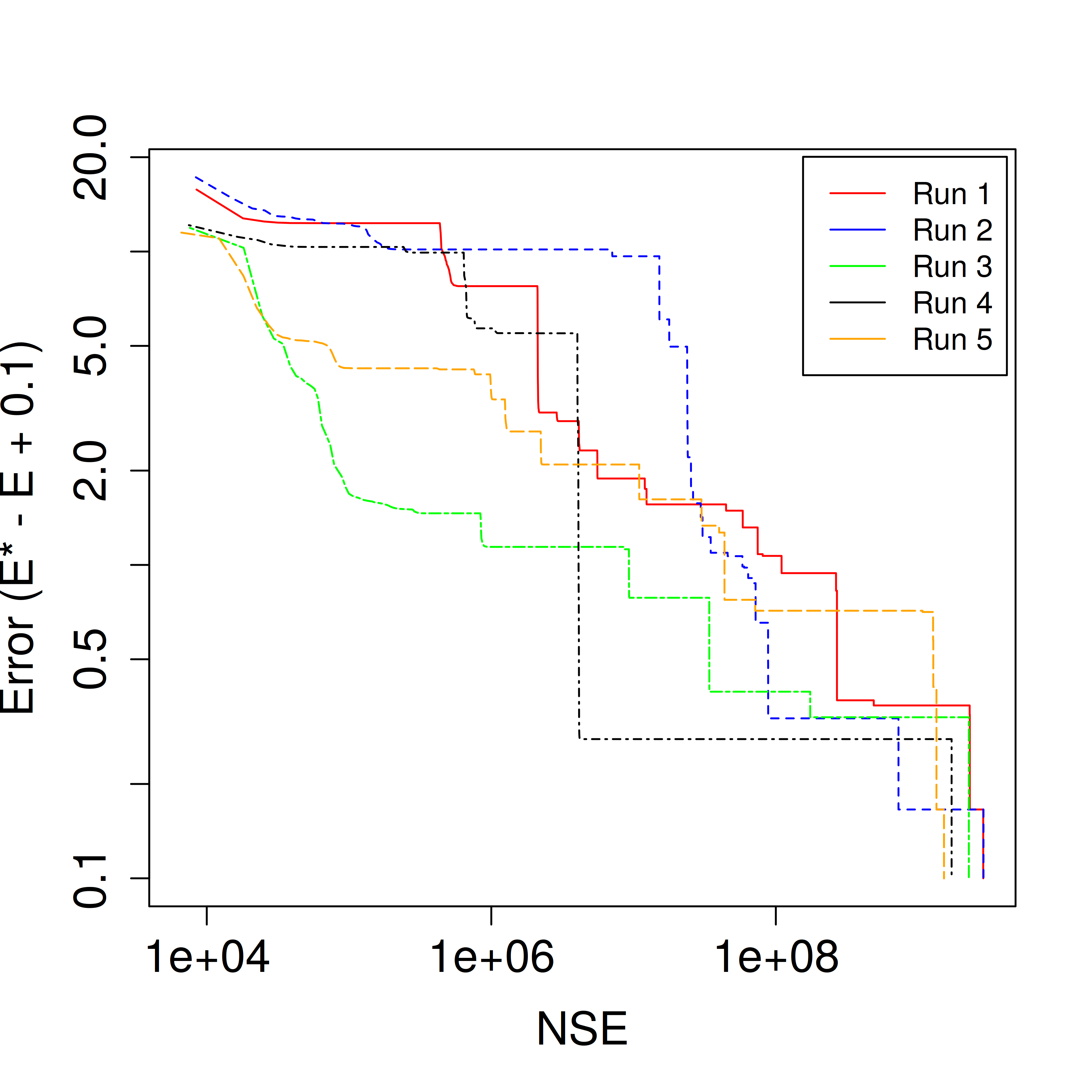
(e) 2ZNF

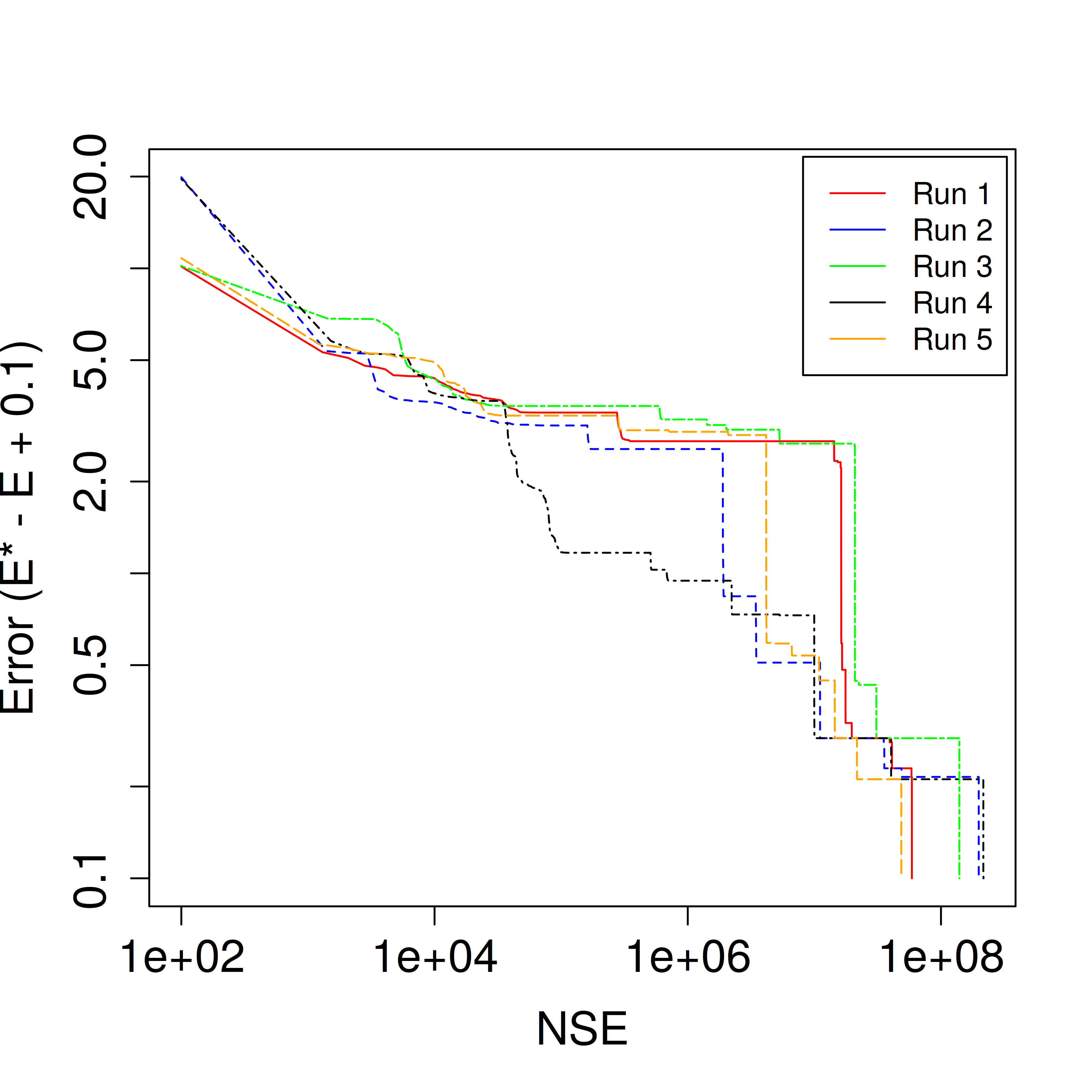
(f) F13

Figure 5: The convergence graphs of the evolutionary process for 5 randomly chosen runs. The error represents the difference between the best-known energy value ($E^{*}$) and the energy value ($E$) of the global best individual within the evolutionary process. A small value of 0.1 was added to the error because of the logarithmic scale.

5.3 Component reinitialization

The main goal of the component reinitialization is to redirect the evolutionary process in such a way that a similar good solution can be located according to the local best solution. To demonstrate the influence of this mechanism on the algorithm’s efficiency, the algorithm was analyzed with (DE${}_{\text{lscr}}$) and without (DE${}_{\text{ls}}$) component reinitialization. Within this analysis, the algorithms were compared using the target values of the best-known energy values and ${\mathit{NSE}}_{\mathit{lmt}}=10^{11}$, as shown in Table 4. The best values of ${\mathit{NSE}}_{\mathit{mean}}$ and $\mathit{hit}_{r}$ are marked in bold typeface. From the results, we can see that the algorithm that uses component reinitialization is capable of reaching the best-known energy value in all runs, and for that it required significantly less solution evaluations (${\mathit{NSE}}$). For example, ${\mathit{NSE}}_{\mathit{mean}}$ was reduced from $1.14$E$+09$ to $8.92$E$+07$ for sequence F13. On the other hand, the algorithm without component reinitialization was not capable of reaching $\mathit{hit}_{r}=100$ within the budget of ${\mathit{NSE}}_{\mathit{lmt}}=10^{11}$ for sequences 1BXL, 1EDP and 2ZNF. From these observations, we can conclude that the proposed component reinitialization allows the algorithm to locate good similar solutions and to reach the best-known energy values. This is shown clearly in Table 4 with $C_{\mathit{NSE}}$ which represents the relationship between the obtained values of ${\mathit{NSE}}_{\mathit{mean}}$ for both algorithms. The component reinitialization reduces the ${\mathit{NSE}}_{\mathit{mean}}$ from 0.38 for sequence 1BXP to less than 0.05 for sequence 2ZNF. Finally, it is obvious that the reinitialization mechanism is responsible for the DE${}_{\text{lscr}}$ obtaining $\mathit{hit}_{r}=100$ for all the sequences shown in Table 4. The convergence curves of 5 randomly chosen runs per sequence are shown in Fig. 5. As we can see, the best-known energy value was reached in all the runs. It is shown with the energy error of 0.1. The energy error represents the difference between the best-known energy value ($E^{*}$) and the energy value ($E$) of the global best individual. Note that, both axes are shown on a logarithmic scale, therefore a small value of 0.1 was added to the energy error.

Results show additionally that the value of ${\mathit{NSE}}_{\mathit{mean}}$ is not only dependent on the sequence length or problem dimension, but also on the sequence itself. For example, for DE${}_{\text{lscr}}$ the value of ${\mathit{NSE}}_{\mathit{mean}}$ is 5.9 times smaller for sequence 2ZNF in comparison with sequence 1BXL, although the dimension of the first sequence is greater than the dimension of the second sequence.

Table 5: Asymptotic average-case performances for DE${}_{\text{lscr}}$. Values marked with the * are obtained by using the grid environment. In these cases $t_{\mathit{mean}}$ is calculated as follows: $t_{\mathit{mean}}=\frac{\mathit{NSE}_{\mathit{mean}}}{v_{\mathit{mean}}}$, where $v_{\mathit{mean}}$ represents the obtained mean speed of three independent runs on our test computer in a given period of time ($t_{\mathit{lmt}}=3600$ seconds). All other results are obtained on our test computer.

Label		1	2	3	4	5	6	7	Asymptotic model
1BXP	$\mathit{target}$	1.8013	2.0063	2.6838	3.1846	4.0191	4.9321	5.6104
	$t_{\mathit{mean}}$	0.16	10.52	395.94	1349.36	12.39	125.70	1965.08	$0.0015\cdot 2.8911^{L}$
	$\mathit{NSE}_{\mathit{mean}}$	2.45E+05	1.38E+07	4.62E+08	1.42E+09	1.17E+07	1.09E+08	1.56E+09	$4589.5644\cdot 2.5970^{L}$
1CB3	$\mathit{target}$	1.9174	1.9786	2.3884	4.0429	6.0209	8.4088	8.4589
	$t_{\mathit{mean}}$	0.06	1.01	1.67	4.22	4.70	80.85	44.47	$0.0001\cdot 2.8662^{L}$
	$\mathit{NSE}_{\mathit{mean}}$	1.03E+05	1.41E+06	2.06E+06	4.82E+06	4.52E+06	7.11E+07	3.61E+07	$344.4917\cdot 2.5502^{L}$
1BXL	$\mathit{target}$	11.1862	13.8397	13.6386	14.0105	16.8991	16.9404	17.3962
	$t_{\mathit{mean}}$	167.93	1472.79	611.86	508.47	25965.63 *	113126.9 *	39706.68 *	$0.0030\cdot 2.7931^{L}$
	$\mathit{NSE}_{\mathit{mean}}$	8.96E+07	7.07E+08	2.68E+08	2.14E+08	9.93E+09 *	4.05E+10 *	1.24E+10 *	$6240.7027\cdot 2.5976^{L}$
1EDP	$\mathit{target}$	6.3823	8.9122	8.7042	9.1152	11.5309	11.7522	15.0092
	$t_{\mathit{mean}}$	677.33	437.82	1280.42	776.01	3494.96	922.22	7272.60	$10.7641\cdot 1.4097^{L}$
	$\mathit{NSE}_{\mathit{mean}}$	6.74E+08	3.88E+08	1.04E+09	5.97E+08	2.47E+09	6.27E+08	4.58E+09	2.32E+07 $\cdot$ 1.3103L
2ZNF	$\mathit{target}$	9.3228	12.1166	11.9772	12.3307	14.6296	14.6733	18.3402
	$t_{\mathit{mean}}$	4153.21	270.26	488.05	755.42	562.56	41844.24 *	7437.15	$16.6030\cdot 1.3505^{L}$
	$\mathit{NSE}_{\mathit{mean}}$	3.67E+09	2.18E+08	3.65E+08	5.50E+08	3.77E+08	1.32E+10 *	2.10E+09	3.19E+07$\cdot 1.2642^{L}$
F13	$\mathit{target}$	1.8225	2.0453	4.6082	4.6858	5.0428	6.8092	6.9961
	$t_{\mathit{mean}}$	0.42	3.34	4.48	8.03	10.47	70.98	110.54	$0.0019\cdot 2.3266^{L}$
	$\mathit{NSE}_{\mathit{mean}}$	6.62E+05	4.52E+06	5.20E+06	8.43E+06	9.74E+06	6.19E+07	8.92E+07	$6138.4492\cdot 2.0846^{L}$

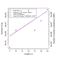
(a) 1BXP

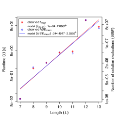
(b) 1CB3

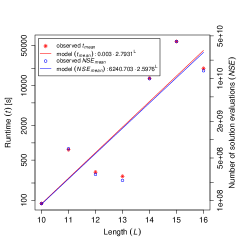
(c) 1BXL

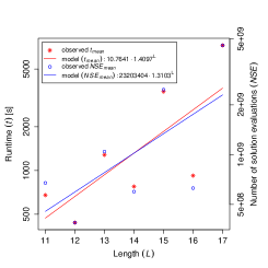
(d) 1EDP

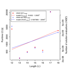
(e) 2ZNF

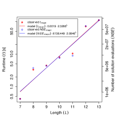
(f) F13

Figure 6: Asymptotic average-case performances for DE${}_{\text{lscr}}$.

5.4 Asymptotic average-case performance

In this section, we introduce an approach to determine asymptotic average-case performance of the algorithm for short sequences. The condition for this is the ability of the algorithm to obtain the best-known solution with $\mathit{hit_{r}}=100$. Until now, only our algorithm has been able to fulfill this condition for the 6 shortest sequences. Six subsequences are generated for each of these sequences. The first subsequence has removed the last monomer, the second subsequence has removed the last two monomers, etc. This means that the length of each next subsequence is decreased by 1. For example, for sequence 1CB3 (BABBBAABBAAAB) the following six subsequences are generated:

• BABBBAABBAAA ($L=12,\mathit{target}=8.4088$),

• BABBBAABBAA ($L=11,\mathit{target}=6.0209$),

• BABBBAABBA ($L=10,\mathit{target}=4.0429$),

• BABBBAABB ($L=9,\mathit{target}=2.3884$),

• BABBBAAB ($L=8,\mathit{target}=1.9786$),

• BABBBAA ($L=7,\mathit{target}=1.9174$).

We determined the best-known or target values for all subsequences. For this purpose, we performed one run for each subsequence with $t_{\mathit{lmt}}=4$ days, and the best reached energy value is used as a target value. Using these target values as a stopping condition, it is possible to calculate asymptotic average-case performance. The original sequence is also included within this calculation. This means the asymptotic average-case performance is determined by using 7 sequences.

Table 5 and Figure 6 display the target values, obtained mean values and asymptotic average-case performances for DE${}_{\text{lscr}}$. From the results, we observe that the best runtime asymptotic average-case performance was obtained for sequence 2ZNF ($16.603\cdot 1.3505^{L}$), while the worst for sequence 1BXP ($0.0015\cdot 2.8911^{L}$). Similarly, the best $\mathit{NSE}$ asymptotic average-case performance was obtained for sequence 2ZNF ($3.19$E$+07\cdot 1.2642^{L}$), while the worst for sequence 1BXL ($6240.7027\cdot 2.5976^{L}$). We can again observe that the value of $\mathit{NSE_{mean}}$ and $\mathit{t_{mean}}$ are not only dependent on the sequence length. Only one monomer can influence these values significantly. For example, DE${}_{\text{lscr}}$ requires less solution evaluations ($\mathit{NSE}$) and runtime ($\mathit{t}$) to reach the target value for the subsequence of sequence 1EDP that has a length of 16 in comparison with a subsequence of length 13. From these results, we can conclude that the structure of the sequence has a big influence on the difficulty of the problem.

Table 6: Comparison of the DE${}_{\text{lscr}}$ algorithm with state-of-the-art algorithms. Entries that are shown as ‘-’ imply that no ‘best energy values’ have been reported in the literature.

Label	$M$	$\mathit{NSE_{lmt}}=M\cdot 10^{4}$									$\mathit{NSE_{lmt}}=M\cdot 10^{4}\cdot c_{v}$
		DE${}_{\text{lscr}}$			DE${}_{\text{pfo}}$ BoskovicAB16			BE-ABC Li15 ; Li15f			DE${}_{\text{lscr}}$
		$E_{\mathit{best}}$	$E_{\mathit{mean}}$	$E_{\mathit{std}}$	$E_{\mathit{best}}$	$E_{\mathit{mean}}$	$E_{\mathit{std}}$	$E_{\mathit{best}}$	$E_{\mathit{mean}}$	$E_{\mathit{std}}$	$E_{\mathit{best}}$	$E_{\mathit{mean}}$	$E_{\mathit{std}}$
1CB3	20	7.7450	4.5108	2.13	8.3690	5.5884	1.96	–	5.9417	0.78	7.7450	4.5929	2.16
1BXL	20	16.2618	12.5045	2.17	16.3443	12.6104	2.53	–	11.6942	1.13	16.7137	13.1940	2.22
1EDP	20	13.1764	8.1986	2.78	13.5620	8.6666	2.56	–	8.0500	0.93	13.1895	8.5313	2.81
2H3S	20	17.1724	11.5310	2.45	16.5030	10.6767	2.75	–	10.4618	1.13	17.4858	11.9565	2.48
2KGU	20	41.0221	33.6539	3.99	44.3369	35.3850	4.70	–	22.7195	2.01	44.0110	36.4642	4.39
1TZ4	20	34.5265	21.6863	3.62	30.9211	20.4361	5.28	–	14.9436	2.22	35.3505	24.9569	4.55
1TZ5	20	37.8896	25.9996	4.12	38.1868	27.3412	4.08	–	17.4859	1.37	40.0161	28.9335	3.60
1AGT	20	49.9861	39.1897	5.21	50.6311	39.0268	5.34	–	25.6024	2.34	54.0897	43.4210	5.45
1CRN	20	74.7849	62.2668	7.60	74.4068	60.2444	7.58	–	42.3083	2.96	82.5999	68.3890	7.28
1HVV	20	45.0054	35.9335	4.92	44.7264	34.8059	5.29	–	21.5386	3.53	57.1990	46.3685	5.61
1GK4	20	49.9316	42.0261	4.77	52.0651	44.8591	4.72	–	27.0410	3.24	69.5798	56.6853	5.16
1PCH	80	121.0579	87.5748	11.42	103.1776	79.4878	8.85	–	51.6674	3.50	128.4882	99.3441	14.52
2EWH	80	193.8143	162.3482	16.60	171.6390	144.9060	12.84	–	94.5785	5.70	210.7021	181.5912	17.49
F13	4	4.9533	3.0907	0.78	5.7290	3.6040	0.66	3.3945	2.8196	0.38	4.9704	3.1977	0.79
F21	4	11.1304	6.5538	1.53	11.2211	7.9567	1.53	6.9065	5.2674	0.76	11.7522	7.6885	1.75
F34	12	19.9550	13.3057	2.47	19.3529	14.0749	2.09	10.4224	8.3239	0.92	21.0345	15.4491	2.85
F55	20	29.5163	22.4019	3.58	31.9554	24.6243	3.57	18.8385	14.4556	1.56	33.1788	26.8111	3.34

5.5 Comparison with other algorithms

In this section, our algorithm is compared with other algorithms according to two stopping conditions $\mathit{NSE_{lmt}}$ and ${\mathit{t_{lmt}}}$, and according to the best obtained energy values.

The obtained results for stopping conditions $\mathit{NSE_{lmt}}$, that were set according to the literature Li15 ; BoskovicAB16 and three algorithms DE${}_{\text{lscr}}$, DE${}_{\text{pfo}}$ and BE-ABC, are shown in Table 6. The best obtained energy values are marked in bold typeface. It can be observed that DE${}_{\text{lscr}}$ and DE${}_{\text{pfo}}$ are comparable, and both outperformed BE-ABC. Results that take into account speed up factor, that are shown in Table 3, are shown in the last column of Table 6. In this case, both algorithms DE${}_{\text{lscr}}$ and DE${}_{\text{pfo}}$ spend approximately the same amount of runtime, and DE${}_{\text{lscr}}$ outperformed DE${}_{\text{pfo}}$ on most sequences. For the sequence 2EWH, the obtained values of $\mathit{E_{mean}}$ were 94.5785, 144.906, 162.3482 and 181.5912 for BE-ABC, DE${}_{\text{pfo}}$, DE${}_{\text{lscr}}$, and DE${}_{\text{lscr}}$ that take into account speed up factor. From these values, it is evident that the proposed algorithm is superior in comparison with BE-ABC and DE${}_{\text{pfo}}$.

Table 7: The obtained results for DE${}_{\text{lscr}}$ and DE${}_{\text{pfo}}$within a runtime limit of 4 days. Entries that are shown as ‘-’ imply that no results have been reported in the literature.

Label	L	DE${}_{\text{lscr}}$, number of independent runs N=100					DE${}_{\text{pfo}}$ BoskovicAB16 , number of independent runs N=30
		$\mathit{E_{best}}$	$\mathit{E_{mean}}$	$\mathit{E_{std}}$	$\mathit{hit_{r}}$		$\mathit{E_{best}}$	$\mathit{E_{mean}}$	$\mathit{E_{std}}$	$\mathit{hit_{r}}$
1BXP	13	5.6104	5.6104	0.0000	100.00		–	–	–	–
1CB3	13	8.4589	8.4589	0.0000	100.00		8.4589	8.4589	0.0000	100.00
1BXL	16	17.3962	17.3962	0.0000	100.00		17.3962	17.1916	0.0878	6.67
1EDP	17	15.0092	15.0092	0.0000	100.00		15.0092	14.9423	0.0471	13.33
2ZNF	18	18.3402	18.3402	0.0000	100.00		–	–	–	–
1EDN	21	21.4703	21.3669	0.0431	7.00		–	–	–	–
2H3S	25	21.1519	20.9956	0.0995	19.00		20.0979	19.6147	0.2699	0.00
1ARE	29	25.2800	24.5444	0.1718	1.00		–	–	–	–
2KGU	34	52.7165	51.7233	0.3829	1.00		50.2960	49.1661	0.6334	0.00
1TZ4	37	43.0229	41.8734	0.4285	1.00		39.7340	37.8329	0.9983	0.00
1TZ5	37	49.3868	48.6399	0.3292	1.00		47.1513	43.9959	1.4087	0.00
1AGT	38	65.1990	64.1285	0.4173	1.00		62.8951	60.4175	1.0439	0.00
1CRN	46	92.9853	89.8223	0.6514	1.00		89.2001	86.0390	1.4529	0.00
2KAP	60	85.5099	83.1503	1.0041	1.00		–	–	–	–
1HVV	75	95.4475	91.4531	1.9215	1.00		82.1427	68.8332	4.0852	0.00
1GK4	84	106.4190	99.6704	3.0377	1.00		90.9140	84.6836	3.3356	0.00
1PCH	88	156.5250	153.1003	2.7117	1.00		131.7787	117.7603	6.2617	0.00
2EWH	98	245.5190	240.2247	2.1421	1.00		225.0968	203.6813	7.1844	0.00
F13	13	6.9961	6.9961	0.0000	100.00		6.9961	6.9961	0.0000	100.00
F21	21	16.5544	16.5304	0.0329	65.00		16.2250	15.8894	0.1849	0.00
F34	34	31.3455	30.4913	0.3458	1.00		28.2509	25.6602	1.0523	0.00
F55	55	51.9030	49.5009	0.8817	1.00		45.0942	41.8670	1.4693	0.00
F89	89	81.5297	76.4804	2.0603	1.00		–	–	–	–

Table 8: Comparisons of the best energy values reported in the literature and the best energy values obtained by DE${}_{\text{lscr}}$. The solution vectors obtained by DE${}_{\text{lscr}}$ are shown in Tables 9 and 10. Entries that shown as ‘-’ imply that no ‘best energy values’ have been reported in the literature.

Label	DE${}_{\text{lscr}}$	DE${}_{\text{pfo}}$	ImHS	BE-ABC	I-PSO	PGATS	MPGPSO	ABC	GATS	C-ABC
		BoskovicAB16	Jana17b	Li15 ; Li15f	Chen11	Zhou14a	Zhou14b	Li14	Wang09 ; Wang11	Wang13
1BXP	5.6104	–	4.498	2.8930	–	–	–	–	–	–
1CB3	8.4589	8.4589	–	8.4580	–	–	–	–	8.2515	–
1BXL	17.3962	17.3962	15.200	15.9261	–	–	–	–	15.8246	–
1EDP	15.0092	15.0092	–	13.9276	–	–	–	–	13.7769	–
2ZNF	18.3402	–	15.056	5.8150	–	–	–	–	–	–
1EDN	21.4703	–	17.721	7.6890	–	–	–	–	–	–
2H3S	21.1519	20.0979	15.340	18.3299	–	–	–	–	18.1640	–
1ARE	25.2800	–	17.416	10.2580	–	–	–	–	–	–
2KGU	52.7165	50.2960	40.696	28.1423	20.9633	32.2599	–	31.9480	–	–
1TZ4	43.0229	39.7340	–	39.4901	–	–	–	–	39.3444	–
1TZ5	49.3868	47.1513	–	45.3233	–	–	–	–	45.3019	–
1AGT	65.1990	62.8951	40.300	51.8019	–	–	–	–	46.0842	–
1CRN	92.9853	89.2001	61.426	54.7253	28.7591	49.6487	43.9339	52.3249	–	–
2KAP	85.5099	–	44.972	27.1400	15.9988	28.1052	18.9513	30.3643	25.1003	–
1HVV	95.4475	82.1427	–	47.4484	–	–	–	–	–	–
1GK4	106.4193	90.9140	–	49.4871	–	–	–	–	–	–
1PCH	156.5252	131.779	–	91.3508	46.4964	49.5729	38.2766	63.4272	–	–
2EWH	245.5193	225.097	–	146.8231	–	–	–	–	–	–
F13	6.9961	6.9961	–	6.9961	–	–	–	–	6.9539	7.0025
F21	16.5544	16.2250	–	15.6258	–	–	–	–	14.7974	14.9570
F34	31.3459	28.2509	–	28.0516	–	–	–	–	27.9897	28.0055
F55	52.0558	45.0942	–	42.5814	–	–	–	–	42.4746	42.2769
F89	83.5761	–	–	–	–	–	–	–	–	–

Within this comparison, the value of $\mathit{NSE_{lmt}}$ was relatively small. This means the reinitialization mechanism did not have a significant impact on the obtained results. Therefore, DE${}_{\text{pfo}}$ and DE${}_{\text{lscr}}$ were also compared according to the ${\mathit{t_{lmt}}}$ that was set to 4 days. A grid environment was used within this comparison and results are shown in Table 7. In this comparison, DE${}_{\text{lscr}}$ obtained better values of $\mathit{E_{mean}}$, $\mathit{E_{best}}$ and $\mathit{hit_{r}}$ in most sequences, and equal values for the shortest sequences. DE${}_{\text{lscr}}$ obtained $\mathit{hit_{r}}$ of 100, 100, 19 and 65 for shorter sequences 1BXL, 1EDP, 2H3S and F21. For the same sequences, DE${}_{\text{pfo}}$ obtained $\mathit{hit_{r}}$ of $6.67,13.33,0$ and $0$, respectively. Significant improvement was obtained for longer sequences too. For example, the best energy values were improved from $90.914,131.7787$ and $225.0968$ to $106.419,156.525$ and $245.519$ for sequences 1GK4, 1PCH and 2EWH, respectively. The energy values were improved by 15.505, 24.7463 and 20.4222. Note that DE${}_{\text{lscr}}$ obtained the new best-known solutions for all sequences with $L\geq 18$, the $\mathit{hit_{r}}=100$ for 6 shortest sequences, and $\mathit{hit_{r}}>1$ for 9 sequences by using $\mathit{t_{lmt}}=4$ days.

The most important results in this paper are shown in Table 8, which collects the best energy values from all experiments that were described in previous sections, and the best-known energy values from the literature. It is evident that DE${}_{\text{lscr}}$ confirmed the best-known energy values for the 3 shortest sequences, and reached the new best-known energy values for all other sequences, except for sequence F13. Solutions for the best energy values reached by DE${}_{\text{lscr}}$ are shown in Tables 9 and 10.

In Kim16 an efficient global optimization method is applied to the sequence F89. Within this work, 32,200 distinct conformations were obtained, and the best obtained energy was 73.1065. DE${}_{\text{lscr}}$ improves this energy by 10.4695, as shown in Table 8.

5.6 Analysis of the obtained structures

For most of the sequences, the best conformations were obtained by using $\mathit{t_{lmt}}=4$ days. Within this experiment, 100 solutions were generated with 100 independent runs. Distribution of the Root-Mean-Square Error (RMSE) values as a function of energy for all these solutions according to the best-known conformation for selected sequences is shown in Fig. 7. Note that the RMSE is calculated by using the superposition between matched pairs. From Fig. 7a, we can see that only two different solutions were reached for sequence 2ZNF. Similar graphs with only two different solutions were obtained for 6 sequences where $\mathit{hit_{r}}=100$ (see Table 7). Three-dimensional representations of these solutions are displayed in Fig. 8. As is shown, for each of these sequences, two solutions are symmetrical according to the XY-plane. This can also be seen from Tables 9 and 10. Two reported solutions for one sequence are very similar. They are different in some components that belong to $\beta$ torsional angles (marked in bold typeface), and their values represent angles with opposite directions. For a little bit longer sequences more different solutions were reached with different energy values, as shown in Figs. 7b and 7c while, for the longest sequences, all 100 solutions are different with different energy values. For example, this is illustrated in Fig. 7d for sequence 2EWH. From these results, we can conclude that all reported symmetrical solutions could be optimal, especially those obtained with $\mathit{hit_{r}}=100$, and all other solutions with $\mathit{hit_{r}}=1$ are almost surely not optimal.

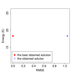
(a) 2ZNF

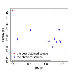
(b) 1EDN

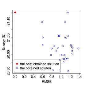
(c) 2H3S

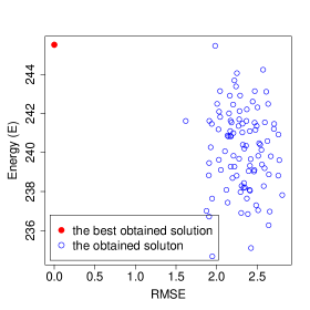
(d) 2EWH

Figure 7: Distribution of the Root-Mean-Square Error (RMSE) values as a function of energy for all 100 obtained conformations within a runtime limit of 4 days, calculated from the best-known conformation.

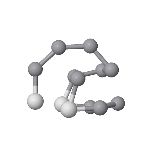
(a) 1BXP

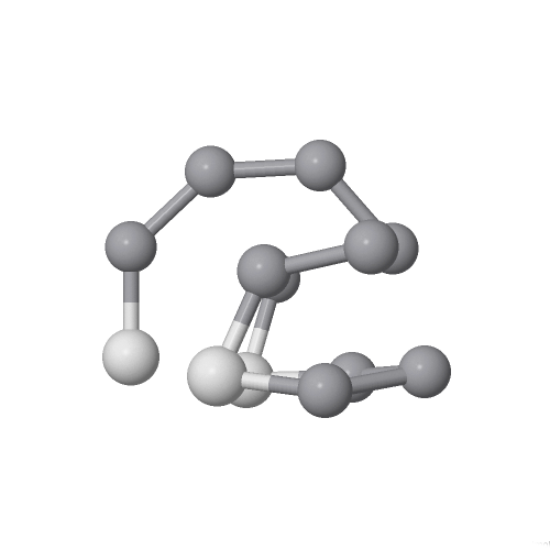
(b) 1BXP

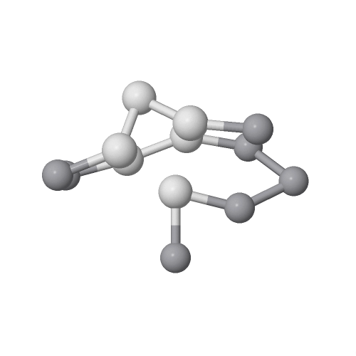
(c) 1CB3

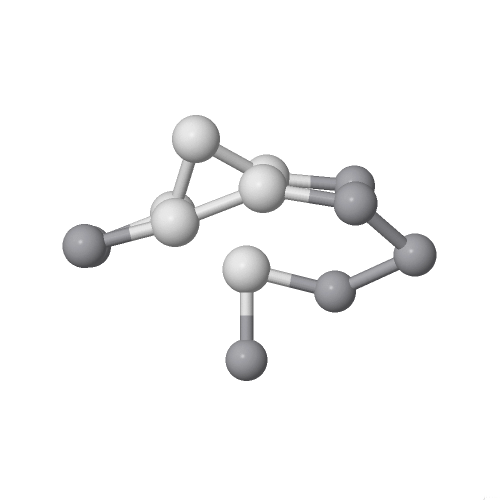
(d) 1CB3

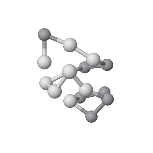
(e) 1BXL

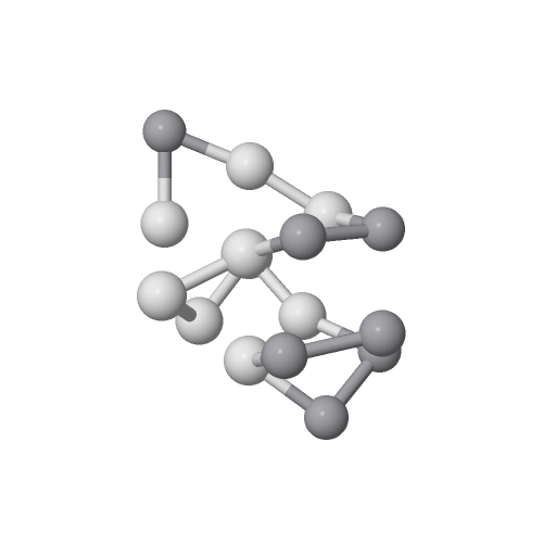
(f) 1BXL

(g) 1EDP

(h) 1EDP

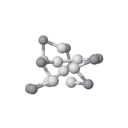
(i) 2ZNF

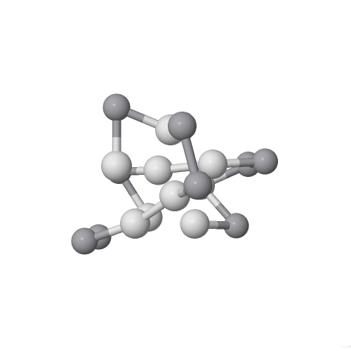
(j) 2ZNF

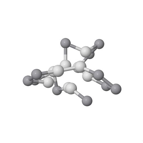
(k) 1EDN

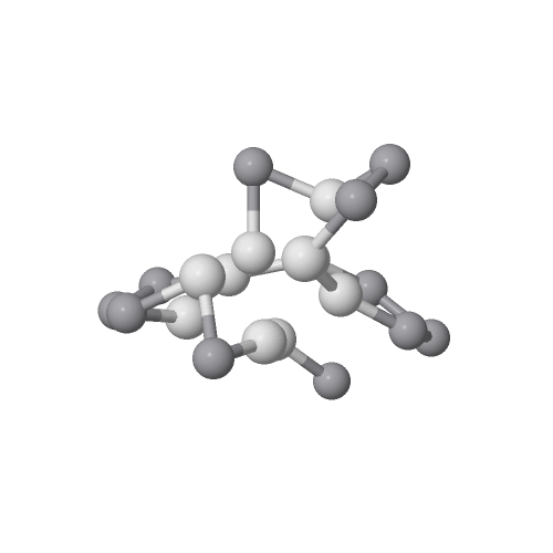
(l) 1EDN

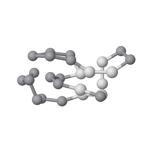
(m) 2H3S

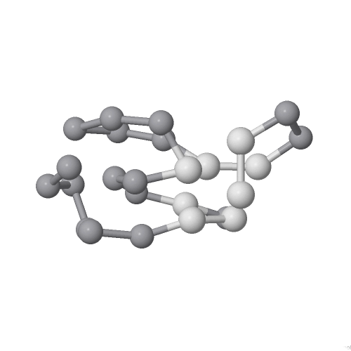
(n) 2H3S

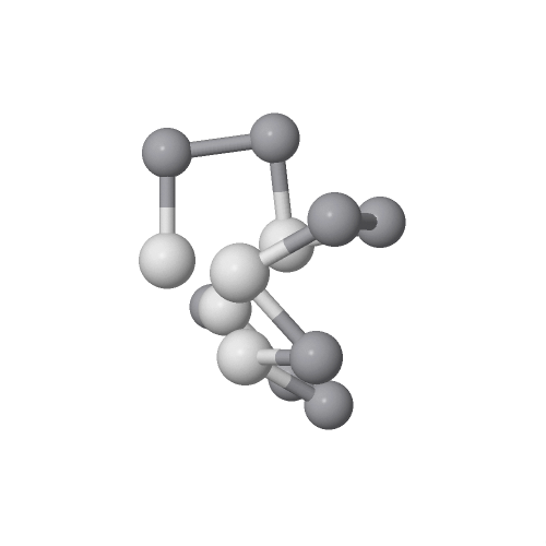
(o) F13

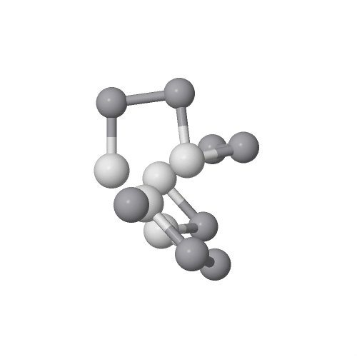
(p) F13

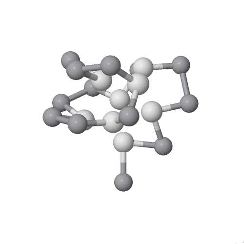
(q) F21

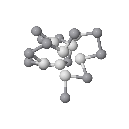
(r) F21

Figure 8: The best obtained conformations that could be optimal.

6 Conclusions

In this paper, we presented a novel Differential Evolution algorithm for protein folding optimization. To improve its efficiency, the algorithm is extended with a component reinitialization and local search that includes a local movement. The component reinitialization is designed to redirect the search process to similar solutions that are different from the already found good solution in only a few components. Thus, the search space around good solutions is explored thoroughly and, consequently, the algorithm can find better solutions. We also designed the local movement for a three-dimen-sional AB off-lattice model in such a way that only a two consecutive monomers are moved locally, while all the remaining monomers remain in their positions. With additional data structure this type of movement allows us to reduce the runtime complexity of the energy calculation within the local search from $\frac{L^{2}}{2}$ to $2L$.

The 23 sequences are used in the experiments to analyze the proposed algorithm and its mechanisms. From the results of the algorithms with and without local search, it is evident that the local movement with additional data structure reduces the runtime complexity of the energy calculation, or increases the number of function evaluations per second by factor 1.46 for the shortest sequences, and by factor 3.91 for the longest sequence. This speed up is dependent on sequence length and the relationship between the number of solution evaluations inside and outside the local search. The local search also improves the algorithm’s convergence speed for most of the sequences. Because of both advantages, the local search improves the efficiency of the algorithm, and this improvement is greater for longer sequences.

Using the best-known energy values as a stopping condition, we demonstrated the usefulness of component reinitialization. It reduces the required mean number of solution evaluations to reach the best-known energy value from 0.38 to less than 0.05. This indicates that the component reinitialization redirects the search process successfully to similar solutions, and allows the algorithm to locate the best-known solutions efficiently.

Our algorithm is the first algorithm that is capable of obtaining a hit ratio of 100% for 6 shorter sequences within the budget of $10^{11}$ function evaluations. Therefore, we introduce an approach for determining asymptotic average-case performances. Our algorithm obtained the best runtime asymptotic average-case performance for sequence 2ZNF ($16.6030\cdot 1.3505^{L}$) and the worst for 1BXP ($0.0015\cdot 2.8911^{L}$). This approach shows additionally that the difficulty of the problem is not only dependent on sequence length, but also on the sequence itself.

The proposed algorithm was also compared with recently published state-of-the-art algorithms for PFO. It outperforms all competitors, and the obtained energy values improve the best-known energy values from the literature for all sequences with $L\geq 18$. For example, the best energy value of sequence 1PCH was improved from 131.7787 to 156.5250 or by 24.7463.

The structure of the best obtained solutions was also analyzed. We figured out that two symmetric best-known solutions exist for sequences with $L\leq 25$. For these sequences, our algorithm obtained a hit ratio equal to or greater than 7%. The solutions of these sequences could be optimal, especially those with a hit ratio of 100%, and solutions for all other sequences are almost surely not optimal.

In the future work we will try to improve the algorithm further by using knowledge about symmetric solutions. This knowledge can be integrated within the evaluation function, or used to reduce the size of the search space. Additionally, we will try to design an algorithm that will reduce the likelihood of the exploration of already explored search space.

Table 9: The best solutions obtained by the DE${}_{\text{lscr}}$ algorithm.

Label	Solution vector in degrees
1BXP	43.2915, 2.88166, -48.728, 0.0655009, 12.6242, 66.0927, -6.40805, 8.96332, 8.80015, 2.23544, 74.0763, -6.62061, 1.31798, -104.099, 160.341, -177.384, -20.6892, 26.8003, 127.789, 166.27, 10.2979
1BXP	43.2915, 2.88166, -48.728, 0.0654961, 12.6242, 66.0927, -6.40805, 8.96332, 8.80016, 2.23544, 74.0763, 6.62061, -1.31798, 104.099, -160.341, 177.384, 20.6892, ${\bf-26.8003}$, -127.789, -166.27, -10.2979
1CB3	-14.0758, 25.2546, -38.7359, -9.58086, 21.0366, 14.7617, -0.998265, 21.5393, 71.2738, -27.6012, -5.16526, -19.1483, -149.775, 172.54, 178.086, 178.164, 91.6772, 4.85452, -31.1093, 28.9806, 3.41538
1CB3	-14.0758, 25.2546, -38.7359, -9.58086, 21.0366, 14.7617, -0.998265, 21.5393, 71.2738, -27.6012, -5.16526, 19.1483, 149.775, -172.54, -178.086, -178.164, -91.6772, -4.85451, 31.1093, -28.9806, -3.41538
1BXL	-22.4292, -32.2737, -16.9254, 5.81295, 15.6175, 26.9979, -38.2372, 52.8361, -48.2442, -24.0736, 49.3335, -36.1178, 13.9215, 12.5486, 1.91872, 55.1452, 147.302, -127.63, 168.592, -62.9624, -27.0891, 28.7221, 27.4283, 152.122, -177.152, 67.7357, -5.21217
1BXL	-22.4292, -32.2737, -16.9254, 5.81296, 15.6175, 26.9979, -38.2372, 52.8361, -48.2442, -24.0736, 49.3335, -36.1178, 13.9215, 12.5486, -1.91872, -55.1452, -147.302, 127.63, -168.592, 62.9624, 27.0891, -28.7221, -27.4283, -152.122, 177.152, -67.7357, 5.21217
1EDP	-22.6336, 7.26974, 60.7674, 23.936, -50.4261, 4.41672, 11.4886, 46.499, 13.2306, $-12.2668$, 22.7087, 4.07035, 30.6245, -69.1251, 16.9542, 26.0209, 124.911, ${\bf-155.575}$, -61.088, 1.55078, 53.7379, 159.421, -162.592, -156.44, -170.499, -85.1224, 2.36332, -25.7677, 67.3571
1EDP	-22.6336, 7.26974, 60.7674, 23.9359, -50.4261, 4.41671, 11.4886, 46.499, 13.2306, $-12.2668$, 22.7087, 4.07036, 30.6245, -69.1251, 16.9542, -26.0209, -124.911, 155.575, 61.088, -1.55077, -53.7379, -159.421, 162.592, 156.44, 170.499, 85.1224, -2.36333, 25.7677, -67.3571
2ZNF	-22.512, 7.71692, -75.1038, 26.0695, 35.539, 19.645, 6.73951, 21.8104, -57.4641, 1.6924, 6.15567, 3.08902, 9.89786, 23.8155, -48.9192, -4.31387, 78.7078, 2.66583, -114.943, -148.187, -162.564, -79.1176, 8.87759, -178.428, 42.9368, 15.8392, -18.6691, -104.193, 166.46, 12.876, 140.107
2ZNF	-22.512 7.71691, -75.1038, 26.0694, 35.539, 19.645, 6.73952, 21.8104, -57.4641, 1.6924, 6.15567, 3.08903, 9.89787, 23.8155, -48.9192, -4.31386, -78.7078, -2.66582, 114.943, 148.187, 162.564, 79.1176, -8.87759, 178.428, -42.9368, -15.8392, 18.6691, 104.193, -166.46, -12.876, -140.107
1EDN	-23.2048, 31.2208, 46.764, 48.9339, -43.6867, -28.0164, -17.6723, -38.3711, -25.1772, 10.6263, 9.07757, 33.5364, -4.83762, -6.09916, 25.0581, -81.151, 15.5944, -3.62479, $-36.6783$, 41.0025, 127.461, -147.732, -53.6249, -22.4102, -68.6344, -166.972, 147.028, -171.451, -155.381, 121.71, 29.6786, 131.144, 15.2983, 24.5428, ${\bf-54.7787}$, -83.2637, -29.6805
1EDN	-23.2048, 31.2207, 46.764, 48.9338, -43.6867, -28.0164, -17.6723, -38.3711, -25.1772, 10.6262, 9.07754, 33.5364, -4.83764, -6.09917, 25.058, -81.151, 15.5944, -3.62479, -36.6783, -41.0025, -127.461, 147.732, 53.6249, 22.4102, 68.6344, 166.972, -147.028, 171.451, 155.381, -121.71, -29.6786, -131.144, -15.2983, -24.5428, 54.7786, 83.2637, 29.6805
2H3S	30.6395, -51.1361, 34.4028, -0.410148, -32.439, -10.4102, -2.09416, 12.4798, -5.74202, -60.0842, 12.6704, -8.68551, -36.5963, -14.4828, -17.9172, 13.0794, 0.148026, 17.7335, -6.06512, 1.46386, -69.7022, 3.0363, 36.2347, -57.1061, -174.679, 173.256, -170.68, -156.724, 142.58, 40.6316, 22.5668, -1.4454, 175.849, -114.818, -61.1893, -4.11275, -27.6809, 84.4735, 144.867, 176.731, 161.605, -97.3254, -158.173, 113.225, 54.3451
2H3S	30.6395, -51.1361, 34.4028, -0.410146, -32.439, -10.4102, -2.09415, 12.4798, -5.74202, -60.0842, 12.6704, -8.68551, -36.5963, -14.4828, -17.9172, 13.0794, 0.148029, 17.7335, -6.06512, 1.46387, -69.7022, 3.0363, 36.2347, 57.1061, 174.679, -173.256, 170.68, 156.724, -142.58, -40.6317, -22.5668, 1.44539, -175.849, 114.818, 61.1893, 4.11273, 27.6808, -84.4735, -144.867, -176.731, -161.605, 97.3254, 158.173, -113.225, -54.3451
1ARE	-11.5547, -1.31888, -15.2569, -42.6589, 17.4763, 5.06218, 14.6442, 24.251, 2.4936, -13.6942, 28.8183, -37.0023, -1.8785, -0.867767, -5.02831, 35.1061, -45.2208, -7.89329, 3.88011, -1.06756, -41.5237, 42.6134, 14.078, 1.71866, -70.4096, 19.7351, 23.088, -23.8173, -48.341, -27.8178, -175.825, 102.429, 138.697, -140.149, -46.4258, -148.917, -22.129, -165.228, 134.775, 48.8091, -12.7742, -50.1159, -163.389, 154.413, 126.397, -131.045, -60.8471, 167.884, 102.299, 52.433, -15.9838, -113.979, -58.9094
2KGU	-156.228, 84.3317, -1.89424, -22.9614, 4.96104, -10.8986, 42.0037, -54.9878, -4.36371, -80.394, 6.84565, -4.01855, -29.0786, 38.404, -24.9304, 51.317, -53.2373, 15.7134, -51.9703, 1.34405, 37.6371, 36.5939, 35.6007, -52.9444, 32.6405, -108.259, -56.7621, 71.7249, 5.9403, 4.99762, 0.0626093, 8.48403, -161.728, -140.31, 137.06, 46.113, 21.1367, 45.0214, -27.4148, 37.097, -8.18763, -148.71, 107.671, -141.471, -176.445, 152.171, -23.7168, -63.0744, -154.472, 9.04166, -89.3673, 21.6149, -71.4051, 41.2427, -22.0274, 113.616, 22.7052, 159.166, -13.0884, -8.78814, 19.7018, 51.7085, 100.664
1TZ4	-13.2782, 2.2117, -21.4873, 13.5614, -50.9456, -18.6314, 58.273, 35.906, -51.557, 43.4606, 14.4093, 26.9361, -9.90087, 51.937, 12.5408, -12.0182, -39.4559, -3.12819, -37.7837, 39.5619, 14.5525, -105.659, -2.39298, 23.2026, 13.2624, 7.00485, -63.913, 21.5608, -2.32347, -4.49988, 14.2846, -2.28795, 25.5405, -52.7743, -3.52791, 88.4618, 172.62, 63.4655, 167.01, -112.19, -129.059, 165.903, 161.114, -13.1829, -29.6599, -142.278, -118.354, -17.9561, 62.8846, 132.227, 150.392, 59.2519, -21.0203, -51.4332, 27.3873, 6.73164, 10.4224, -36.4599, -134.654, -177.842, -46.6888, 152.495, 60.1706, -2.02398, -21.7416, 80.9012, 145.281, -5.47398, -93.0592
1TZ5	19.2916, -25.4743, 37.9748, -2.24909, -71.5607, -62.5534, -1.20914, 60.5119, -37.8385, 56.051, -23.4795, 88.5824, -23.4208, 9.88257, -27.3279, 2.64366, 4.72144, -32.8121, -37.9781, 28.6777, -1.79099, -1.45295, -1.55722, -28.7841, 53.5811, -7.1834, 28.1114, -34.8815, -63.6796, -10.3914, 19.0723, -11.8679, -27.892, -37.0612, 62.2441, 52.8494, -172.157, 163.821, 57.7857, -56.1207, -158.293, 168.377, -23.9122, -20.1987, 4.84453, -2.90382, -36.4027, -130.461, 158.501, 160.429, -146.987, -129.731, 128.236, 34.5188, 28.0746, -55.2047, -137.136, -167.33, 32.699, 35.1309, -64.3505, 35.5609, 22.6136, -27.8717, -112.09, 160.134, -131.465, -173.819, -165.595
1AGT	26.1664, -11.7847, -37.6783, -3.62257, 75.6542, -40.6386, 24.7245, -92.2268, -13.2317, 23.7859, -94.496, -2.2422, 17.0125, 1.77619, -39.6216, 113.613, 89.2441, -4.72246, -98.3805, -65.8427, 44.1904, -17.7537, -84.2295, -2.33273, -55.9952, -46.6065, -1.4073, 40.7682, -24.0458, 37.5641, 44.8005, -1.59772, 9.28805, 12.0621, -52.5228, 21.2213, 120.34, -179.746, -63.7778, 18.8875, 10.4973, -6.76493, -21.1687, 57.2819, 176.355, 27.0186, -122.011, -33.6896, -59.127, -178.6, 14.4172, -4.50249, -165.323, -6.2693, 12.6379, -54.0356, -62.0563, 7.63468, 127.685, 19.1897, 133.256, -157.687, -140.601, -147.971, -19.8046, 48.3979, 166.316, 54.8275, 156.099, 3.00416, -140.869
1CRN	36.2044, -2.8726, -58.3456, -109.168, 67.0176, 63.8303, -34.4202, -9.13991, 27.0952, 6.87578, -175.904, -10.0323, -14.0642, 169.202, 139.54, 37.4324, -30.2161, 3.47033, 120.567, 8.05841, 74.7893, -51.1755, -78.2244, -6.56336, -37.0077, -0.404044, 22.8391, -11.2627, -2.90337, -113.857, -122.645, -5.62342, 80.5936, -19.4761, 87.9704, 12.3212, -4.15216, 3.25955, 39.0676, 30.3454, 61.9086, 12.9802, -97.5976, 8.44839, -76.9107, 30.3312, 41.3065, 24.8161, -34.1801, 20.2024, 33.4227, -14.1966, 80.1988, 28.2782, -166.287, -129.879, -11.8488, 19.3045, -66.9439, -48.3743, -164.938, -12.7803, 7.1584, 29.2233, 12.4003, 39.0045, -58.1443, 52.0717, 43.5443, -0.577219, -103.851, -146.583, -9.20535, -12.6377, -128.769, 27.4049, -32.4672, 16.7912, -135.646, -149.836, 98.1608, 22.2995, 23.6538, 11.9513, 104.699, -3.17593, 35.9215
2KAP	46.469, 9.17062, -12.987, -39.265, -23.0536, 170.718, 7.46538, -139.561, 9.6654, -109.874, 39.7501, -77.1224, -8.16555, 82.4941, -21.6873, 93.4429, -10.6347, 10.7423, 20.8323, -4.45369, -11.4409, -5.20606, 147.482, 172.455, -52.8927, 8.19366, 92.0005, -44.9143, -45.2074, -1.91882, -16.8158, 4.77317, 17.6662, 124.018, 11.9037, -1.64667, 74.9571, 15.2233, -5.48327, -140.99, 19.2716, 15.4203, -48.7429, -34.6525, 5.87344, -6.16017, 41.6324, -16.8426, 49.2516, -28.6507, 29.562, -13.1308, 17.3443, -61.6342, 8.11077, -104.361, 26.4602, 4.19116, 18.9505, 67.8863, 154.188, -116.346, 19.3865, -84.7317, -27.0054, -31.7152, -24.4805, -34.1621, -13.632, 63.0618, 8.2678, -2.60225, 37.1772, -9.33353, -46.953, -117.05, -167.457, 155.733, -103.59, 35.8403, 44.471, -168.41, -18.09, 28.324, 22.7177, -44.4081, -37.3318, -3.25116, 42.16, 57.0729, -4.27289, -157.026, 158.794, -19.8247, 37.3666, 142.492, -5.84281, 168.076, -163.22, -4.06088, -38.3009, 6.22285, -20.4278, 52.41, 156.856, 11.6928, 124.907, -164.531, 100.594, -172.86, -66.3312, -55.802, 13.087, 38.8668, 61.5511

Table 10: The best solutions obtained by the DE${}_{\text{lscr}}$ algorithm.

Label	Solution vector in degrees
1HVV	123.296, 175.071, -104.639, -8.91165, 17.898, 3.71452, 16.7371, -6.98533, -76.7403, -9.21776, 75.2042, 124.487, 46.9457, 18.594, -46.3806, 145.54, 124.742, -1.01034, 2.75056, 10.5349, -7.0204, 118.317, 75.4052, -30.5719, 69.7023, -72.9042, 176.87, -87.9407, -48.7546, 88.4046, -11.7349, 44.1027, -5.14578, -65.6298, 20.3053, -20.9559, -72.1726, 94.427, 45.6623, -45.1943, 55.0226, 121.96, 34.0003, 6.44231, 140.467, 17.4955, 85.266, -21.9109, -95.2265, -24.295, 2.64738, -17.4667, 155.115, -5.99421, -158.933, -6.23019, -43.4673, -28.7354, -11.6413, -19.2361, -10.0374, 34.4593, -178.973, -160.129, -42.443, 5.40211, -87.2981, -36.4155, 10.9084, 64.5935, -5.14139, 28.5554, -18.3091, -3.52734, 45.1155, 9.74914, 114.875, 75.0862, 26.4021, 22.7921, -63.2735, -138.233, -64.6958, -1.96622, 99.8458, -16.8097, 71.6329, 28.1128, -43.4581, -82.0519, 173.534, -96.2117, -16.7565, -32.4898, 48.5607, 11.8749, -64.2088, 1.38784, -57.9374, 25.3469, 54.5768, 34.603, -28.9913, -102.93, -64.0207, -23.3654, 157.688, 118.979, 5.08255, 61.9001, -18.6156, -45.7361, -10.7387, 47.8304, -26.517, -104.738, 22.5679, 115.444, -6.44774, 116.951, 14.5305, -0.364305, 25.7291, 114.23, -22.2869, 97.1472, 0.163606, -93.1095, -14.0922, 67.6929, 103.708, 12.5582, -62.8467, -103.687, -55.8599, 11.7904, 63.4791, 74.9204, 26.812, -72.0632, -116.517, -46.752, 39.4218, 63.2466, 101.367
1GK4	-156.276, -11.1754, -77.6765, -33.983, -9.25845, 27.2496, -22.3371, 55.198, -12.6002, 30.4017, 35.9669, -18.5758, -87.0091, 63.2376, 163.731, -40.6359, 102.397, 146.119, -16.2788, 0.676412, 169.967, -18.769, -43.9974, -62.1645, -51.3378, -148.518, 144.287, -170.774, -25.6785, -22.1326, 27.6078, -8.93322, -75.4448, -68.3403, -16.5373, -128.752, 53.7389, -140.548, -115.598, -1.7515, -106.07, -14.6299, 82.7281, -28.3651, 36.138, 37.748, -23.152, -11.6747, 20.0652, -55.0055, -150.457, -49.5769, 23.078, 65.4316, 111.217, 34.2085, 8.50149, 21.775, -107.598, 139.532, -69.7933, 68.8643, 88.8784, -166.542, -174.708, 31.9934, 137.315, -3.2063, -88.0773, -6.44718, 23.1364, 95.4164, -34.9923, 2.63385, 13.9679, -23.3478, -54.8455, 43.5591, -4.20436, -43.6293, -144.761, 18.6453, 179.845, -29.3419, 34.6059, 116.989, -2.74396, 108.058, 157.394, 13.5671, -34.673, -71.5358, 29.1635, -12.3351, -58.4977, -28.7525, -42.495, -47.6578, 29.0888, -101.645, -92.0769, 10.8024, 101.05, 70.2237, 17.3966, -48.5046, 27.4408, 61.4589, 71.0815, 77.6142, 36.2921, -18.009, -121.503, -122.087, -32.2391, 9.22399, 11.065, 70.686, 48.1796, -38.5792, -91.5736, 15.5793, -173.479, -25.563, 108.153, 54.9784, -50.888, -86.9754, -52.2761, -23.2842, 20.5012, 16.6481, -23.1703, -40.3118, -64.6739, 26.9541, 177.66, 154.029, 125.888, 2.61904, -11.91, -67.2757, 7.45577, 48.5355, -2.84037, -62.5508, -1.94643, 7.24978, 48.2981, 62.3802, 127.482, 80.9534, -6.93496, -105.181, -59.8353, -45.6067, -113.32, 1.58149, -33.4263, -8.31888, 28.5097, -8.75938, 151.901
1PCH	41.1106, -75.4478, -108.35, -88.2808, 52.6905, 63.9346, 98.575, -146.011, -103.251, -81.3915, -7.97873, -5.67391, -138.034, 77.0572, -3.43666, -168.458, -44.1355, -51.9614, -0.548426, -11.6916, -13.85, -90.7331, 162.157, -85.119, -80.3963, 2.41355, -4.42424, 54.2753, 89.5966, -147.035, 78.814, 99.0202, -89.7149, -126.891, -85.1937, 16.9404, -73.4292, 66.5445, 160.832, 40.1368, 145.935, 17.6023, -17.2377, 45.6224, 136.733, -49.815, -43.4151, -102.65, 8.11703, -109.171, -24.407, -47.2699, -132.484, -42.5279, -119.761, 147.911, 73.3968, 3.65598, 74.2541, 19.778, -2.2315, -111.056, -25.0304, -86.2442, 0.146651, 83.5428, -29.3382, 64.0093, 147.03, 73.9582, 29.3652, 154.906, 6.25221, 112.96, 165.03, 11.5624, -48.3887, -130.92, 158.099, -6.47314, -26.6561, -18.5458, -79.5949, 16.5753, 68.4287, 54.4969, 8.59587, -21.8077, -38.0325, -14.1827, -48.149, -7.71342, 5.32628, 34.3591, 4.97453, -19.9588, -29.6581, -39.8474, 152.45, -7.02004, -71.166, 40.6025, 90.9133, 41.1172, 10.2277, -41.2978, -21.4705, -9.53513, 33.3237, -170.287, -147.144, -21.8209, 27.7537, 19.2982, 29.7286, -13.7392, -55.8712, -28.3766, -8.00291, 125.209, 161.205, 19.9805, -46.2199, -2.73427, -12.1052, 106.535, 20.4942, -28.1138, 4.59628, 62.9273, -0.534962, 6.33028, -7.44623, 29.7984, -42.8088, 5.32914, 17.9307, 174.593, -36.0277, 3.2934, 24.3011, 174.231, -1.94325, 107.108, -4.82491, 44.1005, -38.1958, 47.1931, 0.689977, -48.5599, -2.29967, -16.9223, -9.36993, -13.2723, 23.7414, 17.0389, 157.955, 52.6113, 14.0859, -100.053, -42.2958, -9.25703, 37.9416, 58.9846, -28.9415, -56.1025, 37.1207, 50.4847, -55.062
2EWH	151.436, -92.5903, -3.75076, -9.668, -0.975246, 10.9844, 84.1865, -57.1686, 38.7048, 72.7755, 64.7086, 50.2283, 29.5956, -111.649, 163.46, -92.508, -148.929, 61.6607, 124.085, 171.298, -75.5506, -52.2331, -1.37142, -19.9511, 67.108, 14.27, -1.03143, 0.0222875, -116.144, -32.3217, -125.421, -102.86, 145.85, 108.298, -60.4006, -54.4374, -88.1894, -14.6692, 121.958, 125.926, 167.02, -74.5737, -130.938, 62.1354, 106.58, 35.1401, 93.7873, 162.441, 14.5873, -4.93593, 6.27325, -7.31527, 10.8045, -53.8271, -132.021, -37.8517, 30.6805, -89.4307, -61.2859, -31.1104, 90.5217, 118.145, -4.46292, -52.5412, 113.612, 159.141, -3.43442, 62.945, 12.7417, -19.7111, -15.1737, 30.368, -27.5934, -138.544, 7.81197, -59.2248, 9.7981, 122.127, -164.755, 36.2949, 27.611, -37.779, 39.5707, -22.2883, 38.9922, 4.30684, 71.8969, -21.7556, -128.587, -76.5211, -0.480596, 65.3271, 8.48192, 158.34, 107.055, -66.142, 18.5806, -129.465, -18.4294, -11.7806, 50.9098, 132.39, 101.434, 0.100595, -28.2695, 0.622333, 52.5959, 150.715, -11.0556, -45.8273, -39.1155, 8.30602, 56.8165, -46.0845, 17.9186, 11.1667, 19.5044, 89.7449, -23.746, -0.808862, 84.8186, 0.457484, -89.925, -21.9539, 26.9255, -59.9087, 45.3057, -9.74849, -70.462, -14.0544, 18.7807, 59.6121, -176.746, -30.6629, -54.0245, -8.68261, -14.3952, 43.302, 23.9289, 59.5115, -35.76, -58.2711, 2.27009, -152.857, -35.6967, -137.17, -49.407, 36.9083, 58.3246, -26.7135, -71.9911, 26.5305, 53.0114, 52.0147, -21.6699, -14.1031, 12.009, -63.6288, -54.0997, -10.6967, 5.20745, -124.069, -19.2082, 55.6145, -3.07942, 12.0508, 131.359, -177.867, 32.7929, 24.0475, 25.0758, -0.0780254, 5.44473, 36.0356, 28.5948, 22.5261, -174.132, -3.91424, -11.5903, -132.095, -172.313, -25.055, -156.073, 11.1264, 29.3397, -64.3192, -38.8408, -177.009, 22.2676, 11.9142, 56.3727
F13	7.66522, -83.448, 13.0886, 0.55134, 29.1616, -47.908, 2.75327, -31.0327, -31.3119, -46.3918, 0.276218, 9.04884, -29.5745, -116.199, 160.508, 0.890189, 129.381, 24.5074, 113.38, -161.672, 98.7127
F13	7.66522, -83.448, 13.0886, 0.551338, 29.1616, -47.908, 2.75327, -31.0327, -31.3119, -46.3918, 0.276222, -9.04884, 29.5745, 116.199, -160.508, -0.890189, -129.381, -24.5074, -113.38, 161.672, -98.7127
F21	-5.70817, -70.6345, 12.6013, -78.4561, 5.14012, 2.49148, 57.5974, -25.416, 27.2287, -35.8677, -5.33428, -13.9895, 3.02158, 19.9054, 74.4006, -31.0707, 4.76465, -19.1022, -32.9492, 155.506, -16.0013, -169.101, 162.893, -94.9124, 155.503, -140.891, 153.332, 40.6752, 137.563, 48.1957, -35.2245, 66.7533, -37.5734, 137.909, -144.521, -52.7295, -156.871
F21	-5.70816, -70.6345, 12.6014, -78.4561, 5.14014, 2.49149, 57.5974, -25.416, 27.2287, -35.8677, -5.33427, -13.9895, 3.0216, 19.9055, 74.4006, -31.0707, 4.76466, -19.1022, -32.9492, -155.506, 16.0013, 169.101, -162.893, 94.9124, -155.503, 140.891, -153.332, -40.6752, -137.563, -48.1957, 35.2245, -66.7533, 37.5734, -137.909, 144.521, 52.7295, 156.871
F34	12.3298, -83.1718, 20.1532, 8.42606, 37.8998, -37.8448, 9.33408, -77.8143, 7.4245, -73.1774, 26.15, -80.0668, 46.3843, 6.49943, -29.8816, 51.2622, -33.6564, 38.6885, -67.9543, 46.7986, -10.4886, -27.9647, -10.0583, -39.8364, -49.6972, -25.641, 44.7456, -59.6061, 18.6305, -20.9127, 25.4877, 13.4228, 1.77009, 42.1284, 129.207, -149.941, 1.89517, -120.166, 18.4003, 159.01, -168.548, 143.358, 151.62, -49.9323, -164.471, -44.6816, 177.501, -32.6178, 2.86468, -2.00479, -22.1516, -57.0231, -143.09, 131.37, -127.956, 147.157, 57.657, -21.2642, 27.2822, -52.9505, 17.7835, 119.254, 18.7327
F55	-15.6437, 97.9193, 1.00666, 95.3815, 1.86855, -64.0331, -141.452, -2.83476, 104.146, 8.21281, -162.93, -74.3953, 1.96392, 7.65968, -29.2495, 52.5953, 52.8264, -0.624594, 137.07, -4.89079, 0.957561, 150.771, 19.388, 7.34186, 59.4269, 8.22775, -64.6383, -54.8633, -8.8461, 59.752, 162.033, 13.6066, -78.2664, 13.0242, 102.375, 3.23899, -2.60196, -16.3626, 36.9652, -37.8734, 30.0569, 3.86882, -34.6667, -22.5344, 25.3408, 89.0776, 16.5037, -17.6911, -91.108, 4.84917, -9.27247, -4.88184, 6.63221, 4.31554, -28.558, -8.46761, 171.776, -66.1542, 29.7446, -114.307, -0.574113, 83.8969, -5.34284, 64.1091, 6.16523, 112.965, -5.20239, 68.6776, -17.6844, -113.527, 31.5684, -100.963, 152.521, -49.1181, -26.2181, -129.399, -24.1061, 42.4841, -45.0845, 67.3054, -35.1296, 15.741, 34.8919, 33.4461, 7.88754, 179.833, 41.9367, -135.639, 118.444, -156.824, -55.2589, 169.967, 0.172651, 91.1955, -4.02574, -81.307, 23.9152, -29.0528, -154.072, -133.971, 16.3457, -93.6495, -5.71876, 80.2119, -21.5927
F89	179.886, -95.54, -17.2583, -27.4664, -23.3,38.1298, 19.5766, 34.4132, 8.84695, -117.344, -20.5596, -131.943, -11.8962, -48.6976, 129.133, -107.932, 7.29644, 89.0642, 21.8161, 56.2631, -33.6006, -22.3247, -47.5945, -48.8527, -51.6802, 36.4829, 85.1461, 3.54137, 107.149, -0.955333, -51.2341, 65.8004, 13.8676, -69.7918, -0.860014, -134.319, -37.8356, -2.74527, -12.5366, -93.6285, -28.5384, -105.157, 19.0699, 81.6706, 6.93831, 0.887398, 116.484, 23.1153, 132.738, 10.4558, 73.2237, -15.4114, 6.88586, -109.859, -3.3155, -82.7065, 2.76043, -42.4804, 82.5479, -18.3209, -29.9615, -74.7318, -24.0277, 60.1736, -26.3071, -15.531, -14.9412, -79.5093, -1.99245, -48.5295, -70.5006, 58.6443, -42.9465, 50.0326, -70.0616, -9.55698, -109.482, -2.75044, -87.6997, -8.8569, 86.5537, -22.4479, 72.1052, 14.0501, -27.4652, -8.8744, 56.3962, 0.863411, -142.989, -54.5377, 29.0611, -61.1795, 50.3774, -12.8387, 73.4752, 12.0947, -39.6898, -28.42, 143.035, 28.1471, 39.6651, 10.0519, -140.34, -2.35037, 123.344, 3.62448, 125.741, 132.141, 71.1956, -36.3432, -36.7204, -39.5973, 57.8245, -31.8281, 13.6268, -143.946, -36.4178, -6.53297, 34.1645, 12.4669, -82.0619, 14.2377, -32.9623, 49.1945, 137.212, -16.0272, -178.526, 12.3581,69.7334, -1.88293, 147.327, 145.168, 27.4845, -35.3688, 8.48146, -81.2594, -5.25881, 119.388, -139.654, 57.454, 159.88, 27.509, -0.616009, 114.258, -13.2053, -39.494, 65.2585, -42.1881, 0.311959, -22.2436, -162.899, -54.8573, -20.7022, -14.7214, 128.993, 5.42026, 114.069, -21.3562, -46.7891, 18.6434, 15.3431, 121.287, -3.95967, -82.6683, -9.4711, -120.912, -1.33882, -28.956, 43.9338, -42.9642, -139.445, 137.938, 4.62324

References

- (1) Aburomman, A.A., Reaz, M.B.I.: A novel weighted support vector machines multiclass classifier based on differential evolution for intrusion detection systems. Information Sciences 414, 225–246 (2017). doi:10.1016/j.ins.2017.06.007
- (2) Balchin, D., Hayer-Hartl, M., Hartl, F.U.: In vivo aspects of protein folding and quality control. Science 353(6294) (2016). doi:10.1126/science.aac4354
- (3) Bazzoli, A., Tettamanzi, A.G.B.: A Memetic Algorithm for Protein Structure Prediction in a 3D-Lattice HP Model. In: G.R. Raidl, S. Cagnoni, J. Branke, D.W. Corne, R. Drechsler, Y. Jin, C.G. Johnson, P. Machado, E. Marchiori, F. Rothlauf, G.D. Smith, G. Squillero (eds.) Applications of Evolutionary Computing, Lecture Notes in Computer Science, vol. 3005, pp. 1–10. Springer Berlin Heidelberg (2004). doi:10.1007/978-3-540-24653-4_1
- (4) Bošković, B., Brest, J.: Differential evolution for protein folding optimization based on a three-dimensional AB off-lattice model. Journal of Molecular Modeling 22, 1–15 (2016). doi:10.1007/s00894-016-3104-z
- (5) Bošković, B., Brest, J.: Genetic Algorithm with Advanced Mechanisms Applied to the Protein Structure Prediction in a Hydrophobic-Polar Model and Cubic Lattice. Applied Soft Computing 45, 61–70 (2016). doi:10.1016/j.asoc.2016.04.001
- (6) Brest, J., Greiner, S., Bošković, B., Mernik, M., Žumer, V.: Self-Adapting Control Parameters in Differential Evolution: A Comparative Study on Numerical Benchmark Problems. IEEE Trans. Evol. Comput 10(6), 646–657 (2006). doi:10.1109/TEVC.2006.872133
- (7) Buxbaum, E.: Fundamentals of Protein Structure and Function. Springer US (2007)
- (8) Chen, M., Huang, W.q.: Heuristic algorithm for off-lattice protein folding problem. Journal of Zhejiang University SCIENCE B 7(1), 7–12 (2006). doi:10.1631/jzus.2006.B0007
- (9) Chen, X., Lv, M., Zhao, L., Zhang, X.: An Improved Particle Swarm Optimization for Protein Folding Prediction. International Journal of Information Engineering and Electronic Business 3(1), 1–8 (2011). doi:10.5815/ijieeb.2011.01.01
- (10) Das, S., Mullick, S.S., Suganthan, P.: Recent advances in differential evolution – an updated survey. Swarm and Evolutionary Computation 27(Supplement C), 1–30 (2016). doi:10.1016/j.swevo.2016.01.004
- (11) Fraenkel, A.S.: Complexity of protein folding. Bulletin of Mathematical Biology 55(6), 1199–1210 (1993). doi:10.1007/BF02460704
- (12) Hsu, H.P., Mehra, V., Grassberger, P.: Structure optimization in an off-lattice protein model. Phys. Rev. E 68 (2003). doi:10.1103/PhysRevE.68.037703
- (13) Hsu, H.P., Mehra, V., Nadler, W., Grassberger, P.: Growth algorithms for lattice heteropolymers at low temperatures. The Journal of Chemical Physics 118(1), 444–451 (2003). doi:10.1063/1.1522710
- (14) Huang, W., Liu, J.: Structure optimization in a three-dimensional off-lattice protein model. Biopolymers 82(2), 93–98 (2006). doi:10.1002/bip.20400
- (15) Jana, N.D., Sil, J., Das, S.: An Improved Harmony Search Algorithm for Protein Structure Prediction Using 3D Off-Lattice Model, pp. 304–314. Springer Singapore, Singapore (2017). doi:10.1007/978-981-10-3728-3_30
- (16) Jana, N.D., Sil, J., Das, S.: Selection of appropriate metaheuristic algorithms for protein structure prediction in ab off-lattice model: a perspective from fitness landscape analysis. Information Sciences 391–392, 28–64 (2017). doi:10.1016/j.ins.2017.01.020
- (17) Kennedy, D., Norman, C.: Editorial: So much more to know. Science 309, 78–102 (2005). doi:10.1126/science.309.5731.78b
- (18) Kim, J., Straub, J.E., Keyes, T.: Structure optimization and folding mechanisms of off-lattice protein models using statistical temperature molecular dynamics simulation: Statistical temperature annealing. Phys. Rev. E 76 (2007). doi:10.1103/PhysRevE.76.011913
- (19) Kim, S.Y.: Three-dimensional off-lattice ab model protein with the 89-residue fibonacci sequence. Chaos, Solitons & Fractals 90(Supplement C), 111–117 (2016). doi:10.1016/j.chaos.2016.04.010
- (20) Kim, S.Y., Lee, S.B., Lee, J.: Structure optimization by conformational space annealing in an off-lattice protein model. Phys. Rev. E 72 (2005). doi:10.1103/PhysRevE.72.011916
- (21) Li, B., Chiong, R., Lin, M.: A balance-evolution artificial bee colony algorithm for protein structure optimization based on a three-dimensional AB off-lattice model. Computational Biology and Chemistry 54, 1–12 (2015). doi:10.1016/j.compbiolchem.2014.11.004
- (22) Li, B., Lin, M., Liu, Q., Li, Y., Zhou, C.: Protein folding optimization based on 3D off-lattice model via an improved artificial bee colony algorithm. Journal of Molecular Modeling 21(10), 261 (2015). doi:10.1007/s00894-015-2806-y
- (23) Li, Y., Zhou, C., Zheng, X.: The Application of Artificial Bee Colony Algorithm in Protein Structure Prediction. In: L. Pan, G. Păun, M. Pérez-Jiménez, T. Song (eds.) Bio-Inspired Computing - Theories and Applications, Communications in Computer and Information Science, vol. 472, pp. 255–258. Springer Berlin Heidelberg (2014). doi:10.1007/978-3-662-45049-9_42
- (24) Márquez-Chamorroa, A.E., Asencio-Cortésa, G., Santiesteban-Tocab, C.E., Aguilar-Ruiza, J.S.: Soft Computing Methods for the Prediction of Protein Tertiary Structures: A Survey. Applied Soft Computing 35, 398–410 (2015). doi:10.1016/j.asoc.2015.06.024
- (25) Mlakar, U., Potočnik, B., Brest, J.: A hybrid differential evolution for optimal multilevel image thresholding. Expert Systems with Applications 65(Supplement C), 221 – 232 (2016). doi:10.1016/j.eswa.2016.08.046
- (26) Petsko, G., Ringe, D.: Protein Structure and Function. Primers in biology. New Science Press (2004)
- (27) Piotrowski, A.P., Napiorkowski, M.J., Napiorkowski, J.J., Rowinski, P.M.: Swarm intelligence and evolutionary algorithms: Performance versus speed. Information Sciences 384, 34–85 (2017). doi:10.1016/j.ins.2016.12.028
- (28) Stillinger, F.H., Head-Gordon, T., Hirshfeld, C.L.: Toy model for protein folding. Phys. Rev. E 48, 1469–1477 (1993). doi:10.1103/PhysRevE.48.1469
- (29) Storn, R., Price, K.: Differential Evolution - A Simple and Efficient Heuristic for Global Optimization Over Continuous Spaces. J. Glob. Optim. 11(4), 341–359 (1997)
- (30) Tanabe, R., Fukunaga, A.: Improving the search performance of SHADE using linear population size reduction. In: 2014 IEEE Congress on Evolutionary Computation (CEC2014), pp. 1658–1665. IEEE (2014)
- (31) Thachuk, C., Shmygelska, A., Hoos, H.H.: A replica exchange monte carlo algorithm for protein folding in the hp model. BMC Bioinformatics 8(1), 342 (2007). doi:10.1186/1471-2105-8-342
- (32) Wang, T., Zhang, X.: 3D Protein Structure Prediction with Genetic Tabu Search Algorithm in Off-Lattice AB Model. In: Knowledge Acquisition and Modeling, 2009. KAM ’09. Second International Symposium on, vol. 1, pp. 43–46 (2009). doi:10.1109/KAM.2009.2
- (33) Wang, T., Zhang, X.: A case study of 3D protein structure prediction with genetic algorithm and Tabu search. Wuhan University Journal of Natural Sciences 16(2), 125–129 (2011). doi:10.1007/s11859-011-0723-1
- (34) Wang, Y., Guo, G., Chen, L.: Chaotic Artificial Bee Colony algorithm: A new approach to the problem of minimization of energy of the 3D protein structure. Molecular Biology 47(6), 894–900 (2013). doi:10.1134/S0026893313060162
- (35) Wong, K.C., Wu, C.H., Mok, R.K.P., Peng, C., Zhang, Z.: Evolutionary multimodal optimization using the principle of locality. Inf. Sci. 194, 138–170 (2012). doi:10.1016/j.ins.2011.12.016
- (36) Zamuda, A., Brest, J.: Vectorized Procedural Models for Animated Trees Reconstruction using Differential Evolution. Information Sciences 278, 1–21 (2014)
- (37) Zhang, X., Cheng, W.: Protein 3D Structure Prediction by Improved Tabu Search in Off-Lattice AB Model. In: Bioinformatics and Biomedical Engineering, 2008. ICBBE 2008. The 2nd International Conference on, pp. 184–187 (2008). doi:10.1109/ICBBE.2008.50
- (38) Zhou, C., Hou, C., Wei, X., Zhang, Q.: Improved hybrid optimization algorithm for 3D protein structure prediction. Journal of Molecular Modeling 20(7), 2289 (2014). doi:10.1007/s00894-014-2289-2
- (39) Zhou, C., Hu, T., Zhou, S.: Protein Structure Prediction Based on Improved Multiple Populations and GA-PSO. In: L. Pan, G. Păun, M. Pérez-Jiménez, T. Song (eds.) Bio-Inspired Computing - Theories and Applications, Communications in Computer and Information Science, vol. 472, pp. 644–647. Springer Berlin Heidelberg (2014). doi:10.1007/978-3-662-45049-9_105