Scalable Robust Matrix Factorization with Nonconvex Loss

Abstract

Matrix factorization (MF), which uses the $\ell_{2}$-loss, and robust matrix factorization (RMF), which uses the $\ell_{1}$-loss, are sometimes not robust enough for outliers. Moreover, even the state-of-the-art RMF solver (RMF-MM) is slow and cannot utilize data sparsity. In this paper, we propose to improve robustness by using nonconvex loss functions. The resultant optimization problem is difficult. To improve efficiency and scalability, we propose to use the majorization-minimization (MM) and optimize the MM surrogate by using the accelerated proximal gradient algorithm on its dual problem. Data sparsity can also be exploited. The resultant algorithm has low time and space complexities, and is guaranteed to converge to a critical point. Extensive experiments show that it outperforms the state-of-the-art in terms of both accuracy and speed.

1 Introduction

Matrix factorization (MF) is a fundamental tool in machine learning, and an important component in many applications such as computer vision [1, 38], social networks [37] and recommender systems [30]. The square loss has been commonly used in MF [8, 30]. This implicitly assumes the Gaussian noise, and is sensitive to outliers. Eriksson and van den Hengel [12] proposed robust matrix factorization (RMF), which uses the $\ell_{1}$-loss instead, and obtains much better empirical performance. However, the resultant nonconvex nonsmooth optimization problem is much more difficult.

Most RMF solvers are not scalable [6, 12, 22, 27, 40]. The current state-of-the-art solver is RMF-MM [26], which is based on majorization minimization (MM) [20, 24]. In each iteration, a convex nonsmooth surrogate is optimized. RMF-MM is advantageous in that it has theoretical convergence guarantees, and demonstrates fast empirical convergence [26]. However, it cannot utilize data sparsity. This is problematic in applications such as structure from motion [23] and recommender system [30], where the data matrices, though large, are often sparse.

Though the $\ell_{1}$-loss used in RMF is more robust than the $\ell_{2}$, still it may not be robust enough for outliers. Recently, better empirical performance is obtained in total-variation image denosing by using the $\ell_{0}$-loss instead [35], and in sparse coding the capped-$\ell_{1}$ loss [21]. A similar observation is also made on the $\ell_{1}$-regularizer in sparse learning and low-rank matrix learning [16, 38, 41]. To alleivate this problem, various nonconvex regularizers have been introduced. Examples include the Geman penalty [14], Laplace penalty [34], log-sum penalty (LSP) [9] minimax concave penalty (MCP) [39], and the smooth-capped-absolute-deviation (SCAD) penalty [13]. These regularizers are similar in shape to Tukey’s biweight function in robust statistics [19], which flattens for large values. Empirically, they achieve much better performance than $\ell_{1}$ on tasks such as feature selection [16, 41] and image denoising [38].

In this paper, we propose to improve the robustness of RMF by using these nonconvex functions (instead of $\ell_{1}$ or $\ell_{2}$) as the loss function. The resultant optimization problem is difficult, and existing RMF solvers cannot be used. As in RMF-MM, we rely on the more flexible MM optimization technique, and a new MM surrogate is proposed. To improve scalabiltiy, we transform the surrogate to its dual and then solve it with the accelerated proximal gradient (APG) algorithm [2, 32]. Data sparsity can also be exploited in the design of the APG algorithm. As for its convergence analysis, proof techniques in RMF-MM cannot be used as the loss is no longer convex. Instead, we develop new proof techniques based on the Clarke subdifferential [10], and show that convergence to a critical point can be guaranteed. Extensive experiments on both synthetic and real-world data sets demonstrate superiority of the proposed algorithm over the state-of-the-art in terms of both accuracy and scalability.

Notation. For scalar $x$, $\text{sign}\left(x\right)=1$ if $x>0$, 0 if $x=0$, and $-1$ otherwise. For a vector $x$, $\text{Diag}(x)$ constructs a diagonal matrix $X$ with $X_{ii}=x_{i}$. For a matrix $X$, $\|X\|_{F}=(\sum_{i,j}X_{ij}^{2})^{1/2}$ is its Frobenius norm, $\|X\|_{1}=\sum_{i,j}|X_{ij}|$ is its $\ell_{1}$-norm, and $\text{nnz}(X)$ is the number of nonzero elements in $X$. For a square matrix $X$, $\text{tr}(X)=\sum_{i}X_{ii}$ is its trace. For two matrices $X,Y$, $\odot$ denotes element-wise product. For a smooth function $f$, $\nabla f$ is its gradient. For a convex $f$, $G\in\partial f(X)=\{U:f(Y)\geq f(X)+\text{tr}(U^{\top}(Y-X))\}$ is a subgradient.

2 Related Work

2.1 Majorization Minimization

Majorization minimization (MM) is a general technique to make difficult optimization problems easier [20, 24]. Consider a function $h(X)$, which is hard to optimize. Let the iterate at the $k$th MM iteration be $X^{k}$. The next iterate is generated as $X^{k+1}=X^{k}+\arg\min_{X}f^{k}(X;X^{k})$, where $f^{k}$ is a surrogate that is being optimized instead of $h$. A good surrogate should have the following properties [24]: (i) $h(X^{k}+X)\leq f^{k}(X;X^{k})$ for any $X$; (ii) $0=\arg\min_{X}\left(f^{k}(X;X^{k})-h(X^{k}+X)\right)$ and $h(X^{k})=f^{k}(0;X^{k})$; and (iii) $f^{k}$ is convex on $X$. MM only guarantees that the objectives obtained in successive iterations are non-increasing, but does not guarantee convergence of $X^{k}$ [20, 24].

2.2 Robust Matrix Factorization (RMF)

In matrix factorization (MF), the data matrix $M\in\mathbb{R}^{m\times n}$ is approximated by $UV^{\top}$, where $U\in\mathbb{R}^{m\times r}$, $V\in\mathbb{R}^{n\times r}$ and $r\ll\min(m,n)$ is the rank. In applications such as structure from motion (SfM) [1] and recommender systems [30], some entries of $M$ may be missing. In general, the MF problem can be formulated as: $\min_{U,V}\frac{1}{2}\|W\odot(M-UV^{\top})\|_{F}^{2}+\frac{\lambda}{2}(\|U\|_{F}^{2}+\|V\|_{F}^{2})$, where $W\in\{0,1\}^{m\times n}$ contain indices to the observed entries in $M$ (with $W_{ij}=1$ if $M_{ij}$ is observed, and 0 otherwise), and $\lambda\geq 0$ is a regularization parameter. The $\ell_{2}$-loss is sensitive to outliers. In [11], it is replaced by the $\ell_{1}$-loss, leading to robust matrix factorization (RMF):

$$\min_{U,V}\|W\odot(M-UV^{\top})\|_{1}+\frac{\lambda}{2}(\|U\|_{F}^{2}+\|V\|_{F}^{2}).$$ (1)

Many RMF solvers have been developed [7, 12, 18, 6, 22, 26, 27, 40]. However, as the objective in (1) is neither convex nor smooth, these solvers lack scalability, robustness and/or convergence guarantees. Interested readers are referred to Section 2 of [26] for details.

Recently, the RMF-MM algorithm [26] solves (1) using MM. Let the $k$th iterate be $(U^{k},V^{k})$. RMF-MM tries to find increments $(\bar{U},\bar{V})$ that should be added to obtain the target $(U,V)$:

$$U=U^{k}+\bar{U},\quad V=V^{k}+\bar{V}.$$ (2)

Substituting into (1), the objective can be rewritten as $H^{k}(\bar{U},\bar{V})\equiv\|W\odot(M\!-\!(U^{k}+\bar{U})(V^{k}+\bar{V})^{\top})\|_{1}+\frac{\lambda}{2}\|U^{k}+\bar{U}\|_{F}^{2}+\frac{\lambda}{2}\|V^{k}+\bar{V}\|_{F}^{2}$. The following Proposition constructs a surrogate $F^{k}$ of $H^{k}$ that satisfies properties (i) and (ii) in Section 2.1. Unlike $H^{k}$, $F^{k}$ is jointly convex in $(\bar{U},\bar{V})$.

Proposition 2.1.

[26] Let $\text{nnz}(W_{(i,:)})$ (resp. $\text{nnz}(W_{(:,j)})$) be the number of nonzero elements in the $i$th row (resp. $j$th column) of $W$, $\Lambda_{r}=\text{Diag}(\sqrt{\smash[b]{\text{nnz}(W_{(1,:)})}},\dots,\sqrt{\smash[b]{\text{nnz}(W_{(m,:)})}})$, and $\Lambda_{c}=\text{Diag}(\sqrt{\smash[b]{\text{nnz}(W_{(:,1)})}},\dots,\sqrt{\smash[b]{\text{nnz}(W_{(:,n)})}})$. Then, $H^{k}(\bar{U},\bar{V})\leq F^{k}(\bar{U},\bar{V})$, where

$$F^{k}(\bar{U},\bar{V})\equiv \|W\!\odot\!(M-U^{k}(V^{k})^{\top}-\bar{U}(V^{k})^{\top}-U^{k}\bar{V}^{\top})\|_{1}$$

$$+\frac{\lambda}{2}\|U^{k}+\bar{U}\|_{F}^{2}+\frac{1}{2}\|\Lambda_{r}\bar{U}\|_{F}^{2}+\frac{\lambda}{2}\|V^{k}+\bar{V}\|_{F}^{2}+\frac{1}{2}\|\Lambda_{c}\bar{V}\|_{F}^{2}.$$ (3)

Equality holds iff $(\bar{U},\bar{V})=(0,0)$.

Because of the coupling of $\bar{U},V^{k}$ (resp. $U^{k},\bar{V}$) in $\bar{U}(V^{k})^{\top}$ (resp. $U^{k}\bar{V}^{\top}$) in (3), $F^{k}$ is still difficult to optimize. To address this problem, RMF-MM uses the LADMPSAP algorithm [25], which is a multi-block variant of the alternating direction method of multipliers (ADMM) [3].

RMF-MM has a space complexity of $O(mn)$, and a time complexity of $O(mnrIK)$, where $I$ is the number of (inner) LADMPSAP iterations and $K$ is the number of (outer) RMF-MM iterations. These grow linearly with the matrix size, and can be expensive on large data sets. Besides, as discussed in Section 1, the $\ell_{1}$-loss may still be sensitive to outliers.

3 Proposed Algorithm

3.1 Use a More Robust Nonconvex Loss

In this paper, we improve robustness of RMF by using a general nonconvex loss instead of the $\ell_{1}$-loss. Problem (1) is then changed to:

$$\min_{U,V}\dot{H}(U,V)\equiv\sum_{i=1}^{m}\sum_{j=1}^{n}W_{ij}\phi\left(|M_{ij}-[UV^{\top}]_{ij}|\right)+\frac{\lambda}{2}(\|U\|_{F}^{2}+\|V\|_{F}^{2}),$$ (4)

where $\phi$ is nonconvex. We assume the following on $\phi$:

Assumption 1.

$\phi(\alpha)$ is concave, smooth and strictly increasing on $\alpha\geq 0$.

Assumption 1 is satisfied by many nonconvex functions, including the Geman, Laplace and LSP penalties mentioned in Section 1, and slightly modified variants of the MCP and SCAD penalties. Details can be found in Appendix A. Unlike previous papers [16, 41, 38], we use these nonconvex functions as the loss, not as regularizer. The $\ell_{1}$ also satisfies Assumption 1, and thus (4) includes (1).

When the $i$th row of $W$ is zero, the $i$th row of $U$ obtained is zero because of the $\|U\|_{F}^{2}$ regularizer. Similarly, when the $i$th column of $W$ is zero, the corresponding column in $V$ is zero. To avoid this trivial solution, we make the following Assumption, which is also used in matrix completion [8] and RMF-MM.

Assumption 2.

$W$ has no zero row or column.

3.2 Constructing the Surrogate

Problem (4) is difficult to solve, and existing RMF solvers cannot be used as they rely crucially on the $\ell_{1}$-norm. In this Section, we use the more flexible MM technique as in RMF-MM. However, its surrogate construction scheme cannot be used here. RMF-MM uses the convex $\ell_{1}$ loss, and only needs to handle nonconvexity resulting from the product $UV^{\top}$ in (1). Here, nonconvexity in (4) comes from both from the loss and $UV^{\top}$.

The following Proposition first obtains a convex upper bound of the nonconvex $\phi$ using Taylor expansion. An illustration is shown in Figure 1. Note that this upper bound is simply a re-weighted $\ell_{1}$, with scaling factor $\phi^{\prime}(|\beta|)$ and offset $\phi(|\beta|)-\phi^{\prime}(|\beta|)|\beta|$. As one may expect, recovery of the $\ell_{1}$ makes optimization easier. It is known that the LSP, when used as a regularizer, can be interpreted as re-weighted $\ell_{1}$ regularization [8]. Thus, Proposition 3.1 includes this as a special case.

Proposition 3.1.

For any given $\beta\in\mathbb{R}$, $\phi(|\alpha|)\leq\phi^{\prime}(|\beta|)|\alpha|+(\phi(|\beta|)-\phi^{\prime}(|\beta|)|\beta|)$, and the equality holds iff $\alpha=\pm\beta$.

(a) Geman.

(b) Laplace.

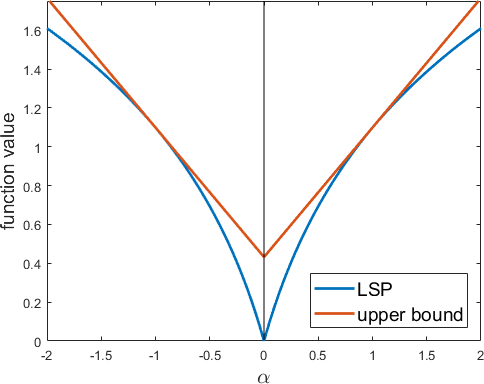
(c) LSP.

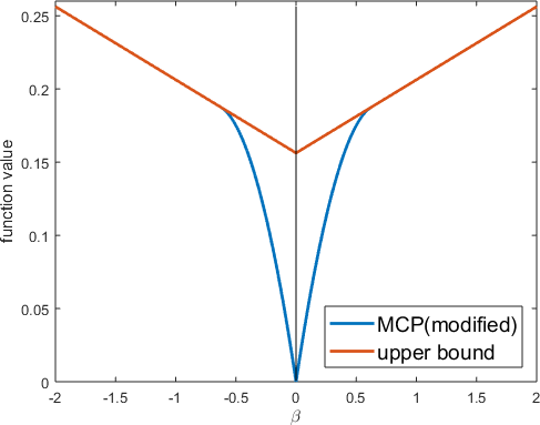
(d) modified MCP.

(e) modified SCAD.

Figure 1: Upper bounds for the various nonconvex penalities (see Table 5 in Appendix A.2) $\beta=1$, $\theta=2.5$ for SCAD and $\theta=0.5$ for the others; and $\delta=0.05$ for MCP and SCAD.

Given the current iterate $(U^{k},V^{k})$, we want to find increments $(\bar{U},\bar{V})$ as in (2). $\dot{H}$ in (4) can be rewritten as: $\dot{H}^{k}(\bar{U},\bar{V})\equiv\sum_{i=1}^{m}\sum_{j=1}^{n}W_{ij}\phi(|M_{ij}-[(U^{k}\!+\bar{U})(V^{k}+\bar{V})^{\top}]_{ij}|)+\frac{\lambda}{2}\|U^{k}+\bar{U}\|_{F}^{2}+\frac{\lambda}{2}\|V^{k}+\bar{V}\|_{F}^{2}$. Using Proposition 3.1, we obtain the following convex upper bound for $\dot{H}^{k}$.

Corollary 3.2.

$\dot{H}^{k}(\bar{U},\bar{V})\leq b^{k}+\frac{\lambda}{2}\|U^{k}+\bar{U}\|_{F}^{2}+\frac{\lambda}{2}\|V^{k}+\bar{V}\|_{F}^{2}+\|\dot{W}^{k}\odot(M-U^{k}(V^{k})^{\top}-\bar{U}(V^{k})^{\top}-U^{k}\bar{V}^{\top}-\bar{U}\bar{V}^{\top})\|_{1}$, where $b^{k}=\sum_{i=1}^{m}\sum_{j=1}^{n}W_{ij}(\phi(|[U^{k}(V^{k})^{\top}]_{ij}|)-A^{k}_{ij}|[U^{k}(V^{k})^{\top}]_{ij}|)$, $\dot{W}^{k}$ $=A^{k}\odot W$, and $A^{k}_{ij}=\phi^{\prime}(|[U^{k}(V^{k})^{\top}]_{ij}|)$.

The product $\bar{U}\bar{V}^{\top}$ still couples $\bar{U}$ and $\bar{V}$ together. As $\dot{H}^{k}$ is similar to $H^{k}$ in Section 2.2, one may want to reuse Proposition 2.1. However, Proposition 2.1 holds only when $W$ is a binary matrix, while $\dot{W}^{k}$ here is real-valued. Let $\Lambda_{r}^{k}=\text{Diag}(\sqrt{\smash[b]{\text{sum}(\dot{W}_{(1,:)}^{k})}},\dots,\sqrt{\smash[b]{\text{sum}(\dot{W}_{(m,:)}^{k})}})$ and $\Lambda_{c}^{k}=\text{Diag}(\sqrt{\smash[b]{\text{sum}(\dot{W}_{(:,1)}^{k})}},\dots,\sqrt{\smash[b]{\text{sum}(\dot{W}_{(:,n)}^{k})}})$. The following Proposition shows that $\dot{F}^{k}(\bar{U},\bar{V})\equiv\|\dot{W}^{k}\odot(M-U^{k}(V^{k})^{\top}-\bar{U}(V^{k})^{\top}-U^{k}\bar{V}^{\top})\|_{1}+\frac{\lambda}{2}\|U^{k}+\bar{U}\|_{F}^{2}+\frac{1}{2}\|\Lambda_{r}^{k}\bar{U}\|_{F}^{2}+\frac{\lambda}{2}\|V^{k}+\bar{V}\|_{F}^{2}+\frac{1}{2}\|\Lambda_{c}^{k}\bar{V}\|_{F}^{2}+b^{k}$, can be used as a surrogate. Moreover, it can be easily seen that $\dot{F}^{k}$ qualifies as a good surrogate in Section 2.1: (a) $\dot{H}(\bar{U}+U^{k},\bar{V}+V^{k})\leq\dot{F}^{k}(\bar{U},\bar{V})$; (b) $(0,0)=\arg\min_{\bar{U},\bar{V}}\dot{F}^{k}(\bar{U},\bar{V})-\dot{H}^{k}(\bar{U},\bar{V})$ and $\dot{F}^{k}(0,0)=\dot{H}(0,0)$; and (c) $\dot{F}^{k}$ is jointly convex in $\bar{U},\bar{V}$.

Proposition 3.3.

$\dot{H}^{k}(\bar{U},\bar{V})\leq\dot{F}^{k}(\bar{U},\bar{V})$, with equality holds iff $(\bar{U},\bar{V})=(0,0)$.

Remark 3.1.

In the special case where the $\ell_{1}$-loss is used, $\dot{W}^{k}=W$, $b^{k}=0$ $\Lambda_{r}^{k}=\Lambda_{r}$, and $\Lambda_{c}^{k}=\Lambda_{c}$. The surrogate $\dot{F}^{k}(\bar{U},\bar{V})$ then reduces to that in (3), and Proposition 3.3 becomes Proposition 2.1.

3.3 Optimizing the Surrogate via APG on the Dual

LADMPSAP, which is used in RMF-MM, can also be used to optimize $\dot{F}^{k}$. However, the dual variable in LADMPSAP is a dense matrix, and cannot utilize possible sparsity of $W$. Moreover, LADMPSAP converges at a rate of $O(1/T)$ [25], which is slow. In the following, we propose a time- and space-efficient optimization procedure basesd on running the accelerated proximal gradient (APG) algorithm on the surrogate optimization problem’s dual. Note that while the primal problem has $O(mn)$ variables, the dual problem has only $\text{nnz}(W)$ variables.

3.3.1 Problem Reformulation

Let $\Omega\equiv\{(i_{1},j_{1}),\dots,(i_{\text{nnz}(W)},j_{\text{nnz}(W)})\}$ be the set containing indices of the observed elements in $W$, $\mathcal{H}_{\Omega}(\cdot)$ be the linear operator which maps a $\text{nnz}(W)$-dimensional vector $x$ to the sparse matrix $X\in\mathbb{R}^{m\times n}$ with nonzero positions indicated by $\Omega$ (i.e., $X_{i_{t}j_{t}}=x_{t}$ where $(i_{t},j_{t})$ is the $t$th element in $\Omega$), and $\mathcal{H}_{\Omega}^{-1}(\cdot)$ be the inverse operator of $\mathcal{H}_{\Omega}$.

Proposition 3.4.

The dual problem of $\min_{\bar{U},\bar{V}}\dot{F}^{k}(\bar{U},\bar{V})$ is

$$\min_{x\in\mathcal{W}^{k}}\mathcal{D}^{k}(x) \equiv \frac{1}{2}\text{tr}((\mathcal{H}_{\Omega}(x)V^{k}-\lambda U^{k})^{\top}A_{r}^{k}(\mathcal{H}_{\Omega}(x)V^{k}-\lambda U^{k}))-\text{tr}(\mathcal{H}_{\Omega}(x)^{\top}M)$$ (5)

$$+\frac{1}{2}\text{tr}((\mathcal{H}_{\Omega}(x)^{\top}U^{k}-\lambda V^{k})^{\top}A_{c}^{k}(\mathcal{H}_{\Omega}(x)^{\top}U^{k}-\lambda V^{k})),$$

where $\mathcal{W}^{k}\equiv\{x\in\mathbb{R}^{\text{nnz}(W)}:|x_{i}|\leq[\dot{w}^{k}]_{i}^{-1}\}$, $\dot{w}^{k}=\mathcal{H}_{\Omega}^{-1}(\dot{W}^{k})$, $A_{r}^{k}=(\lambda I+(\Lambda_{r}^{k})^{2})^{-1}$, and $A_{c}^{k}=(\lambda I+(\Lambda_{c}^{k})^{2})^{-1}$. From the obtained $x$, the primal $(\bar{U},\bar{V})$ solution can be recovered as $\bar{U}=A_{r}^{k}(\mathcal{H}_{\Omega}(x)V^{k}-\lambda U^{k})$ and $\bar{V}=A_{c}^{k}(\mathcal{H}_{\Omega}(x)^{\top}U^{k}-\lambda V^{k})$.

Problem (5) can be solved by the APG algorithm, which has a convergence rate of $O(1/T^{2})$ [2, 32] and is faster than LADMPSAP. As $\mathcal{W}^{k}$ involves only $\ell_{1}$ constraints, the proximal step can be easily computed with closed-form (details are in Appendix B.3) and takes only $O(\text{nnz}(W))$ time.

The complete procedure, which will be called Robust Matrix Factorization with Nonconvex Loss (RMFNL) algorithm is shown in Algorithm 1. The surrogate is optimized via its dual in step 4. The primal solution is recovered in step 5, and $(U^{k},V^{k})$ are updated in step 6.

Algorithm 1 Robust matrix factorization using nonconvex loss (RMFNL) algorithm.

1:  initialize $U^{1}\in\mathbb{R}^{m\times r}$ and $V^{1}\in\mathbb{R}^{m\times r}$;

2:  for $k=1,2,\dots,K$ do

3:     compute $\dot{W}^{k}$ in Corollary 3.2 (only on the observed positions), and $\Lambda_{r}^{k},\Lambda_{c}^{k}$;

4:     compute $x^{k}=\arg\min_{x\in\mathcal{W}^{k}}\mathcal{D}^{k}(x)$ in Proposition 3.4 using APG;

5:     $\bar{U}^{k}=A_{r}^{k}\left(\mathcal{H}_{\Omega}(x^{k})V^{k}-\lambda U^{k}\right)$,   $\bar{V}^{k}=A_{c}^{k}(\mathcal{H}_{\Omega}(x^{k})^{\top}U^{k}-\lambda V^{k})$;

6:     $U^{k+1}=U^{k}+\bar{U}^{k}$,   $V^{k+1}=V^{k}+\bar{V}^{k}$;

7:  end for

8:  return  $U^{K+1}$ and $V^{K+1}$.

3.3.2 Exploiting Sparsity

A direct implementation of APG takes $O(mn)$ space and $O(mnr)$ time per iteration. In the following, we show how these can be reduced by exploiting sparsity fo $W$.

The objective in (5) involves $A_{r}^{k},A_{c}^{k}$ and $\mathcal{W}^{k}$, which are all related to $\dot{W}^{k}$. Recall that $\dot{W}^{k}$ in Corollary 3.2 is sparse (as $W$ is sparse). Thus, by exploting sparsity, constructing $A_{r}^{k},A_{c}^{k}$ and $\mathcal{W}^{k}$ only take $O(\text{nnz}(W))$ time and space.

In each APG iteration, one has to compute the gradient, objective, and proximal step. First, consider the gradient $\nabla\mathcal{D}^{k}(x)$ of the objective, which is equal to

$$\mathcal{H}_{\Omega}^{\!-\!1}(A_{r}^{k}(\mathcal{H}_{\Omega}(x)V^{k}-\lambda U^{k})(V^{k})^{\top})+\mathcal{H}_{\Omega}^{\!-\!1}(U^{k}[(U^{k})^{\top}\mathcal{H}_{\Omega}(x)-\lambda(V^{k})^{\top}]A_{c}^{k})-\mathcal{H}_{\Omega}^{\!-\!1}(M).\!\!\!\!$$ (6)

The first term can be rewritten as $\hat{g}^{k}=\mathcal{H}_{\Omega}^{\!-\!1}(Q^{k}(V^{k})^{\top})$, where $Q^{k}=A_{r}^{k}(\mathcal{H}_{\Omega}(x)V^{k}-\lambda U^{k})$. As $A_{r}^{k}$ is diagonal and $\mathcal{H}_{\Omega}(x)$ is sparse, $Q^{k}$ can be computed as $A_{r}^{k}(\mathcal{H}_{\Omega}(x)V^{k})-\lambda(A_{r}^{k}U^{k})$ in $O(\text{nnz}(W)r+mr)$ time, where $r$ is the number of columns in $U^{k}$ and $V^{k}$. Let the $t$th element in $\Omega$ be $(i_{t},j_{t})$. By the definition of $\mathcal{H}_{\Omega}^{\!-\!1}(\cdot)$, we have $\hat{g}^{k}_{t}=\sum_{q=1}^{r}Q^{k}_{i_{t}q}V^{k}_{j_{t}q}$, and this takes $O(\text{nnz}(W)r+mr)$ time. Similarly, computing the second term in (6) takes $O(\text{nnz}(W)r+nr)$ time. Hence, computing $\nabla\mathcal{D}^{k}(x)$ takes a total of $O(\text{nnz}(W)r+(m+n)r)$ time and $O(\text{nnz}(W)+(m+n)r)$ space (the Algorithm is shown in Appendix B.1). Similarly, the objective can be obtained in $O(\text{nnz}(W)r+(m+n)r)$ time and $O(\text{nnz}(W)+(m+n)r)$ space (details are in Appendix B.2). The proximal step takes $O(\text{nnz}(W))$ time and space, as $x\in\mathbb{R}^{\text{nnz}(W)}$. Thus, by exploiting sparsity, the APG algorithm has a space complexity of $O(\text{nnz}(W)+(m+n)r)$ and iteration time complexity of $O(\text{nnz}(W)r+(m+n)r)$. In comparison, LADMPSAP needs $O(mn)$ space and iteration time complexity of $O(mnr)$. A summary of the complexity results is shown in Figure 2(a).

3.4 Convergence Analysis

In this section, we study the convergence of RMFNL. Note that the proof technique in RMF-MM cannot be used, as it relies on convexity of the $\ell_{1}$-loss while $\phi$ in (4) is nonconvex (in particular, Proposition 1 in [26] fails). Moreover, the proof of RMF-MM uses the subgradient. Here, as $\phi$ is nonconvex, we will use the Clarke subdifferential [10], which generalizes subgradients to nonconvex functions (a brief introduction is in Appendix C). For the iterates $\{X^{k}\}$ generated by RMF-MM, it is guaranteed to have a sufficient decrease on the objective $f$ in the following sense [26]: There exists a constant $\gamma>0$ such that $f(X^{k})-f(X^{k+1})\geq\gamma\|X^{k}-X^{k+1}\|_{F}^{2},\forall k$. The following Proposition shows that RMFNL also achieves a sufficient decrease on its objective. Moreover, the $\{(U^{k},V^{k})\}$ sequence generated is bounded, which has at least one limit point.

Proposition 3.5.

For Algorithm 1, $\{(U^{k},V^{k})\}$ is bounded, and has a sufficient decrease on $\dot{H}$.

Theorem 3.6.

The limit points of the sequence generated by Algorithm 1 are critical points of (4).

4 Experiments

In this section, we compare the proposed RMFNL with state-of-the-art MF algorithms. Experiments are performed on a PC with Intel i7 CPU and 32GB RAM. All the codes are in Matlab, with sparse matrix operations implemented in C++. We use the nonconvex loss functions of LSP, Geman and Laplace in Table 5 of Appendix A, with $\theta=1$; and fix $\lambda=20/(m+n)$ in (1) as suggested in [26].

4.1 Synthetic Data

We first perform experiments on synthetic data, which is generated as $X=UV^{\top}$ with $U\in\mathbb{R}^{m\times 5}$, $V\in\mathbb{R}^{m\times 5}$, and $m=\{250,500,1000\}$. Elements of $U$ and $V$ are sampled i.i.d. from the standard normal distribution $\mathcal{N}(0,1)$. This is then corrupted to form $M=X+N+S$, where $N$ is the noise matrix from $\mathcal{N}(0,0.1)$, and $S$ is a sparse matrix modeling outliers with 5% nonzero elements randomly sampled from $\{\pm 5\}$. We randomly draw $10\log(m)/m\%$ of the elements from $M$ as observations, with half of them for training and the other half for validation. The remaining unobserved elements are for testing. Note that the larger the $m$, the sparser is the observed matrix.

The iterate $(U^{1},V^{1})$ is initialized as Gaussian random matrices, and the iterative procedure is stopped when the relative change in objective values between successive iterations is smaller than $10^{-4}$. For the subproblems in RMF-MM and RMFNL, iteration is stopped when the relative change in objective value is smaller than $10^{-6}$ or when a maximum of $300$ iterations is used. The rank $r$ is set to the ground truth (i.e., 5). For performance evaluation, we follow [26] and use the (i) testing root mean square error, $\text{RMSE}=\sqrt{\smash[b]{\|\bar{W}\odot(X-\bar{U}\bar{V}^{T})\|_{F}^{2}/\text{nnz}(\bar{W})}}$, where $\bar{W}$ is a binary matrix indicating positions of the testing elements; and (ii) CPU time. To reduce statistical variability, results are averaged over five repetitions.

4.1.1 Solvers for Surrogate Optimization

Here, we compare three solvers for surrogate optimization in each RMFNL iteration (with the LSP loss and $m=1000$): (i) LADMPSAP in RMF-MM; (ii) APG(dense), which uses APG but without utilizing data sparsity; and (iii) APG in Algorithm 1, which utilizes data sparsity as in Section 3.3. The APG stepsize is determined by line-search, and adaptive restart is used for further speedup [32]. Figure 2 shows convergence in the first RMFNL iteration (results for the other iterations are similar). As can be seen, LADMPSAP is the slowest w.r.t. the number of iterations, as its convergence rate is inferior to both variants of APG (whose rates are the same). In terms of CPU time, APG is the fastest as it can also utilize data sparsity.

(a) Complexities of surrogate optimizers.

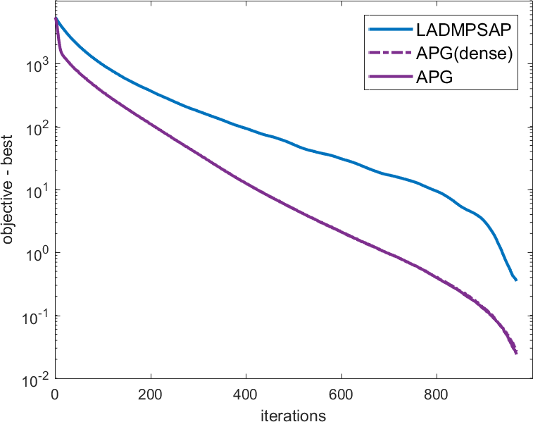
(b) Number of iterations.

(c) CPU time.

Figure 2: Convergence of the objective on the synthetic data set (with the LSP loss and $m=1000$). Note that the curves for APG-dense and APG overlap in Figure 2(b).

Table 1 shows performance of the whole RMFNL algorithm with different surrogate optimizers. As can be seen, the various nonconvex losses (LSP, Geman and Laplace) lead to similar RMSE’s, as has been similarly observed in [16, 38]. Moreover, the different optimizers all obtain the same RMSE. In terms of speed, APG is the fastest, then followed by APG(dense), and LADMPSAP is the slowest. Hence, in the sequel, we will only use APG to optimize the surrogate.

Table 1: Performance of RMFNL with different surrogate optimizers.

		$m=250$ (nnz: 11.04%)		$m=500$ (nnz: 6.21%)		$m=1000$ (nnz: 3.45%)
loss	solver	RMSE	CPU time	RMSE	CPU time	RMSE	CPU time
	LADMPSAP	0.110$\pm$0.004	17.0$\pm$1.4	0.072$\pm$0.001	195.7$\pm$34.7	0.45$\pm$0.007	950.8$\pm$138.8
LSP	APG(dense)	0.110$\pm$0.004	12.1$\pm$0.6	0.073$\pm$0.001	114.4$\pm$18.8	0.45$\pm$0.007	490.1$\pm$91.9
	APG	0.110$\pm$0.004	3.2$\pm$0.6	0.073$\pm$0.001	5.5$\pm$1.0	0.45$\pm$0.006	24.6$\pm$3.2
	LADMPSAP	0.115$\pm$0.014	20.4$\pm$0.8	0.074$\pm$0.006	231.0$\pm$36.9	0.45$\pm$0.007	950.8$\pm$138.8
Geman	APG(dense)	0.115$\pm$0.011	13.9$\pm$1.6	0.073$\pm$0.002	146.9$\pm$24.8	0.45$\pm$0.007	490.1$\pm$91.9
	APG	0.114$\pm$0.009	3.1$\pm$0.5	0.073$\pm$0.002	8.3$\pm$1.1	0.45$\pm$0.006	24.6$\pm$3.2
	LADMPSAP	0.110$\pm$0.004	17.1$\pm$1.5	0.072$\pm$0.001	203.4$\pm$22.7	0.45$\pm$0.007	950.8$\pm$138.8
Laplace	APG(dense)	0.110$\pm$0.004	12.1$\pm$2.1	0.073$\pm$0.003	120.9$\pm$28.9	0.45$\pm$0.007	490.1$\pm$91.9
	APG	0.111$\pm$0.004	2.8$\pm$0.4	0.074$\pm$0.001	5.6$\pm$1.0	0.45$\pm$0.006	24.6$\pm$3.2

4.1.2 Comparison with State-of-the-Art Matrix Factorization Algorithms

Next, we compare RMFNL with state-of-the-art MF and RMF algorithms. The $\ell_{2}$-loss-based MF algorithms that will be compared include alternating gradient descent (AltGrad) [30], Riemannian preconditioning (RP) [29], scaled alternating steepest descent (ScaledASD) [33], alternative minimization for large scale matrix imputing (ALT-Impute) [17] and online massive dictionary learning (OMDL) [28]. The $\ell_{1}$-loss-based RMF algorithms being compared include RMF-MM [26], robust matrix completion (RMC) [7] and Grassmannian robust adaptive subspace tracking algorithm (GRASTA) [18]. Codes are provided by the respective authors. We do not compare with AOPMC [36], which has been shown to be slower than RMC [7].

As can be seen from Table 2, RMFNL produces much lower RMSE than the MF/RMF algorithms, and the RMSEs from different nonconvex losses are similar. AltGrad, RP, ScaledASD, ALT-Impute and OMDL are very fast because they use the simple $\ell_{2}$ loss. However, their RMSEs are much higher than RMFNL and RMF algorithms. A more detailed convergence comparison is shown in Figure 3. As can be seen, RMF-MM is the slowest. RMFNL with different nonconvex losses have similar convergence behavior, and they all converge to a lower testing RMSE much faster than the others.

Table 2: Performance of the various matrix factorization algorithms on synthetic data.

		$m=250$ (nnz: 11.04%)		$m=500$ (nnz: 6.21%)		$m=1000$ (nnz: 3.45%)
loss	algorithm	RMSE	CPU time	RMSE	CPU time	RMSE	CPU time
$\ell_{2}$	AltGrad	1.062$\pm$0.040	1.0$\pm$0.6	0.950$\pm$0.005	1.8$\pm$0.3	0.853$\pm$0.010	6.0$\pm$4.2
	RP	1.048$\pm$0.071	0.1$\pm$0.1	0.953$\pm$0.012	0.4$\pm$0.2	0.848$\pm$0.009	1.1$\pm$0.1
	ScaledASD	1.042$\pm$0.066	0.2$\pm$0.1	0.950$\pm$0.009	0.4$\pm$0.3	0.847$\pm$0.009	1.2$\pm$0.5
	ALT-Impute	1.030$\pm$0.060	0.2$\pm$0.1	0.937$\pm$0.010	0.3$\pm$0.1	0.838$\pm$0.009	1.0$\pm$0.2
	OMDL	1.089$\pm$0.055	0.1$\pm$0.1	0.945$\pm$0.018	0.2$\pm$0.1	0.847$\pm$0.009	0.5$\pm$0.2
$\ell_{1}$	GRASTA	0.338$\pm$0.033	1.5$\pm$0.1	0.306$\pm$0.002	2.9$\pm$0.3	0.244$\pm$0.009	6.1$\pm$0.4
	RMC	0.226$\pm$0.040	2.8$\pm$1.0	0.201$\pm$0.001	2.7$\pm$0.5	0.195$\pm$0.006	4.2$\pm$2.5
	RMF-MM	0.194$\pm$0.032	13.4$\pm$0.6	0.145$\pm$0.009	154.9$\pm$12.5	0.122$\pm$0.004	827.7$\pm$116.3
LSP	RMFNL	0.110$\pm$0.004	3.2$\pm$0.6	0.073$\pm$0.001	5.5$\pm$1.0	0.047$\pm$0.002	14.0$\pm$5.2
Geman	RMFNL	0.114$\pm$0.004	3.1$\pm$0.5	0.073$\pm$0.001	8.3$\pm$1.1	0.047$\pm$0.001	19.0$\pm$4.9
Laplace	RMFNL	0.111$\pm$0.004	2.8$\pm$0.4	0.074$\pm$0.001	5.6$\pm$1.0	0.047$\pm$0.002	15.9$\pm$6.1

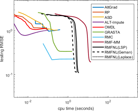
(a) $m=250$.

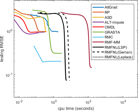
(b) $m=500$.

(c) $m=1000$.

Figure 3: Convergence of testing RMSE for the various algorithms on synthetic data.

4.2 Robust Collaborative Recommendation

In a recommender system, the love/hate attack changes the ratings of selected items to the minimum (hate) or maximum (love) [5]. The love/hate attack is very simple, but can significantly bias overall prediction. As no love/hate attack data sets are publicly available, we follow [5, 31] and manually add permutations. Experiments are performed on the popular MovieLens recommender data sets: MovieLens-100K, MovieLens-1M, and MovieLens-10M (Some statistics on these data sets are in Appendix E.1). We randomly select 3% of the items from each data set. For each selected item, all its observed ratings are set to either the minimum or maximum with equal possibilities. $50\%$ of the observed ratings are used for training, $25\%$ for validation, and the rest for testing. Algorithms in Section 4.1.1 will be compared. To reduce statistical variability, results are averaged over five repetitions. As in Section 4.1, the testing RMSE and CPU time are used for performance evaluation.

Results are shown in Table 3, and Figure 4 shows convergence of the RMSE. Again, RMFNL with different nonconvex losses have similar performance and achieve the lowest RMSE. The MF algorithms are fast, but have high RMSEs. GRASTA is not stable, with large RMSE and variance.

Table 3: Performance on the MovieLens data sets. CPU time is in seconds. RMF-MM cannot converge in $10^{4}$ seconds on the MovieLens-1M and MovieLens-10M data sets, and thus is not reported.

		MovieLens-100K		MovieLens-1M		MovieLens-10M
loss	algorithm	RMSE	CPU time	RMSE	CPU time	RMSE	CPU time
$\ell_{2}$	AltGrad	0.954$\pm$0.004	1.0$\pm$0.2	0.856$\pm$0.005	30.6$\pm$2.5	0.872$\pm$0.003	1130.4$\pm$9.6
	RP	0.968$\pm$0.008	0.2$\pm$0.1	0.867$\pm$0.002	4.4$\pm$0.4	0.948$\pm$0.011	199.9$\pm$39.0
	ScaledASD	0.951$\pm$0.004	0.3$\pm$0.1	0.878$\pm$0.003	8.7$\pm$0.2	0.884$\pm$0.001	230.2$\pm$7.7
	ALT-Impute	0.942$\pm$0.021	0.2$\pm$0.1	0.859$\pm$0.001	10.7$\pm$0.2	0.872$\pm$0.001	198.9$\pm$2.6
	OMDL	0.958$\pm$0.003	0.1$\pm$0.1	0.873$\pm$0.008	2.6$\pm$0.5	0.881$\pm$0.003	63.4$\pm$4.2
$\ell_{1}$	GRASTA	1.057$\pm$0.218	4.6$\pm$0.3	0.842$\pm$0.011	31.1$\pm$0.6	0.876$\pm$0.047	1304.3$\pm$18.0
	RMC	0.920$\pm$0.001	1.4$\pm$0.2	0.849$\pm$0.001	40.6$\pm$2.2	0.855$\pm$0.001	526.0$\pm$29.5
	RMF-MM	0.901$\pm$0.003	402.3$\pm$80.0	—	—	—	—
LSP	RMFNL	0.885$\pm$0.006	5.9$\pm$1.5	0.828$\pm$0.001	34.9$\pm$1.0	0.817$\pm$0.004	1508.2$\pm$69.1
Geman	RMFNL	0.885$\pm$0.005	6.6$\pm$1.2	0.829$\pm$0.005	35.3$\pm$0.3	0.817$\pm$0.004	1478.5$\pm$72.8
Laplace	RMFNL	0.885$\pm$0.005	4.9$\pm$1.1	0.828$\pm$0.001	35.1$\pm$0.2	0.817$\pm$0.005	1513.4$\pm$12.2

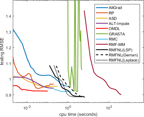
(a) MovieLens-100K.

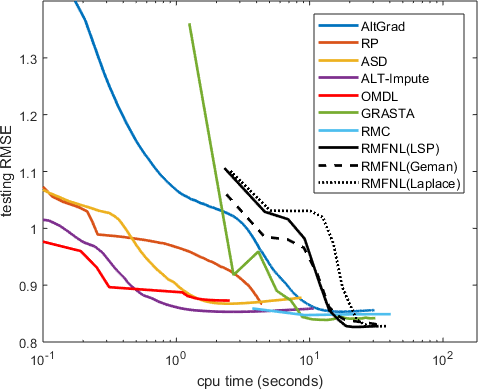
(b) MovieLens-1M.

(c) MovieLens-10M.

Figure 4: Convergence of testing RMSE on the recommendation data sets.

4.3 Affine Rigid Structure-from-Motion (SfM)

SfM reconstructs the 3D scene from sparse feature points tracked in $m$ images of a moving camera [23]. Each feature point is projected to every image plane, and is thus represented by a $2m$-dimensional vector. With $n$ feature points, this leads to a $2m\times n$ matrix. Often, this matrix has missing data (e.g., some feature points may not be always visible) and outliers (arising from feature mismatch). We use the Oxford Dinosaur sequence, which has $36$ images and $4,983$ feature points. As in [26], we extract three data subsets using feature points observed in at least $5,6$ and $7$ images. These are denoted “D1" (with size 72$\times$932), “D2" (72$\times$557) and “D3" (72$\times$336). The fully observed data matrix can be recovered by rank-$4$ matrix factorization [12], and so we set $r=4$.

We compare RMFNL with RMF-MM and its variant (denoted RMF-MM(heuristic)) described in Section 4.2 of [26]. In this variant, the diagonal entries of $\Lambda_{r}$ and $\Lambda_{c}$ are initialized with small values and then increased gradually. It is claimed in [26] that this leads to faster convergence. However, our experimental results show that this heuristic leads to more accurate, but not faster, results. Moreover, the key pitfall of this variant is that Proposition 2.1 and the convergence guarantee for RMF-MM no longer holds.

For performance evaluation, as there is no ground-truth, we follow [26] and use the (i) mean absolute error (MAE) $\|\bar{W}\odot(\bar{U}\bar{V}^{\top}-X)\|_{1}/\text{nnz}(\bar{W})$, where $\bar{U}$ and $\bar{V}$ are outputs from the algorithm, $X$ is the data matrix with observed positions indicated by the binary $\bar{W}$; and (ii) CPU time. As the various nonconvex penalties have been shown to have similar performance, we will only report the LSP here.

Results are shown in Table 4. As can be seen, RMF-MM(heuristic) obtains a lower MAE than RMF-MM, but is still outperformed by RMFNL. RMFNL is the fastest, though the speedup is not as significant as in previous sections. This is because the Dinosaur subsets are not very sparse (the percentages of nonzero entries in “D1", “D2" and “D3" are $17.9\%$, $20.5\%$ and $23.1\%$, respectively).

Table 4: Performance on the Dinosaur data subsets. CPU time is in seconds.

	D1		D2		D3
	MAE	CPU time	MAE	CPU time	MAE	CPU time
RMF-MM(heuristic)	0.374$\pm$0.031	43.9$\pm$3.3	0.381$\pm$0.022	25.9$\pm$3.1	0.382$\pm$0.034	10.8$\pm$3.4
RMF-MM	0.442$\pm$0.096	26.9$\pm$3.4	0.458$\pm$0.043	14.9$\pm$2.2	0.466$\pm$0.072	9.2$\pm$2.1
RMFNL	0.323$\pm$0.012	8.3$\pm$1.9	0.332$\pm$0.005	6.8$\pm$1.3	0.316$\pm$0.006	3.4$\pm$1.0

5 Conclusion

In this paper, we improved the robustness of matrix factorization by using a nonconvex loss instead of the commonly used (convex) $\ell_{1}$ and $\ell_{2}$-losses. Second, we improved its scalabililty by exploiting data sparsity (which RMF-MM cannot) and using the accelerated proximal gradient algorithm (which is faster than the commonly used ADMM). The space and iteration time complexities are greatly reduced. Theoretical analysis shows that the proposed RMFNL algorithm generates a critical point. Extensive experiments on both synthetic and real-world data sets demonstrate that RMFNL is more accurate and more scalable than the state-of-the-art.

Acknowledgment

The first author would like to specially thanks for Weiwei Tu and Yuqiang Chen from 4Paradigm Inc.

Appendix A Nonconvex Functions

A.1 Modification of MCP and SCAD

For the minimax concave penalty (MCP) [39]:

$$\phi(|\alpha|)=\begin{cases}|\alpha|-\frac{\alpha^{2}}{2\theta}&|\alpha|\leq\theta\\ \frac{1}{2}\theta&|\alpha|>\theta\end{cases}.$$

MCP does not meet Assumption 1 as $\phi$ is not strictly increasing when $|\alpha|>\theta$. To avoid this problem, we can simply modify its $\phi$ as $\tilde{\phi}(|\alpha|)=\phi(|\alpha|)+\delta|\alpha|$, where $\delta>0$ is a small constant (Figure 1(d)). The smoothly clipped absolute deviation (SCAD) penalty [13] can be modified in the same way (Figure 1(e)).

A.2 Definitions

A formal definition of nonconvex functions can be used by RMFML is in Table 5.

Table 5: Example nonconvex regularizers ($\theta>2$ for SCAD and $\theta>0$ for others is a constant). Here, $\delta>0$ is a small constant to ensure that the $\phi$’s for MCP and SCAD are strictly increasing.

	$\phi(|\alpha|)$
Geman penalty	$\frac{|\alpha|}{\theta+|\alpha|}$
Laplace penalty	$1-\exp\left(-\frac{|\alpha|}{\theta}\right)$
log-sum-penalty (LSP)	$\log\left(1+\frac{|\alpha|}{\theta}\right)$
minimax concave penalty (MCP)	$\begin{cases}(1+\delta)|\alpha|-\frac{\alpha^{2}}{2\theta}&\alpha\leq\theta\\ \frac{1}{2}\theta^{2}+\delta|\alpha|&\alpha>\theta\end{cases}$
smoothly clipped absolute deviation (SCAD) penalty	$\begin{cases}(1+\delta)|\alpha|&|\alpha|\leq 1\\ \frac{-\alpha^{2}+2\theta|\alpha|-1}{2(\theta-1)}+\delta|\alpha|&1<|\alpha|\leq\theta\\ \frac{(1+\theta)}{2}+\delta|\alpha|&|\alpha|>\theta\end{cases}$

Appendix B Details of the APG Algorithm

B.1 Computing the Gradient

The complete procedure for computing the gradient is shown in Algorithm 2.

Algorithm 2 Computing $\nabla\mathcal{D}^{k}(x)$ by exploiting sparsity.

1:  set $X_{i_{t}j_{t}}=x_{t}$ for all $(i_{t},j_{t})\in\Omega$; // i.e., $X=\mathcal{H}_{\Omega}(x)$

2:  $Q^{k}=A_{r}^{k}(XV^{k})-\lambda(A_{r}^{k}U^{k})$;

3:  obtain $\hat{g}^{k}\in\mathbb{R}^{\text{nnz}(W)}$ with $\hat{g}^{k}_{t}=\sum_{q=1}^{r}Q^{k}_{i_{t}q}V^{k}_{j_{t}q}$;

4:  $P^{k}=A_{c}^{k}(X^{\top}U^{k})-\lambda(A_{c}^{k}V^{k})$;

5:  obtain $\breve{g}^{k}\in\mathbb{R}^{\text{nnz}(W)}$ with $\breve{g}^{k}_{t}=\sum_{q=1}^{r}U^{k}_{i_{t}q}P^{k}_{j_{t}q}$;  // i.e., $\breve{g}^{k}=\mathcal{H}_{\Omega}^{\!-\!1}(U^{k}(P^{k})^{\top})$

6:  return  $\hat{g}^{k}+\breve{g}^{k}-\mathcal{H}_{\Omega}^{\!-\!1}(M)$.

B.2 Computing the Objective

By the definition of $\mathcal{H}_{\Omega}(x)$, we construct a sparse matrix $X=\mathcal{H}_{\Omega}(x)$. We then compute the first term in (5) as $\frac{1}{2}\|P^{k}\sqrt{A_{r}^{k}}\|_{F}^{2}$ where $P^{k}=XV^{k}-\lambda U^{k}$. Note that $X$ is sparse with $O(\text{nnz}(W))$ nonzero elements and $A_{r}^{k}$ is a diagonal, the computation of the first term in (5) takes $O(\text{nnz}(W)r+mr)$ time, where $r$ is the number of columns in $U^{k}$. Let $y=\mathcal{H}_{\Omega}^{\!-\!1}(M)$. The second term in (5) can then be computed as $\sum_{i=1}^{\text{nnz}(W)}x_{i}y_{i}$, which takes $O(\text{nnz}(W))$ time. For the last term in (5), it can be computed similarly as the first term using $O(\text{nnz}(W)r+nr)$ time. Moreover, we can see that only $O(\text{nnz}(W)+(m+n)r)$ space is needed.

The whole procedure for computing the objective is shown in Algorithm 3. It takes $O(\text{nnz}(W)+(m+n)r)$ space and $O(\text{nnz}(W)r+(m+n)r)$ time in total.

Algorithm 3 Computing $\mathcal{D}^{k}(x)$ by exploiting sparsity.

1:  set $X_{i_{t}j_{t}}=x_{t}$ for all $(i_{t},j_{t})\in\Omega$;

2:  $a_{1}=\frac{1}{2}\|\sqrt{A_{r}^{k}}P^{k}\|_{F}^{2}$ where $P^{k}=XV^{k}-\lambda U^{k}$;

3:  $a_{2}=\frac{1}{2}\|\sqrt{A_{c}^{k}}Q^{k}\|_{F}^{2}$ where $Q^{k}=X^{\top}U^{k}-\lambda V^{k}$;

4:  $a_{3}=\sum_{i=1}^{\text{nnz}(W)}x_{i}y_{i}$ where $y=\mathcal{H}_{\Omega}^{\!-\!1}(M)$;

5:  return  $a_{1}+a_{2}+a_{3}$.

B.3 Computing the Proximal Step

For the proximal step with (5), a closed-form solution can be obtained by the following Lemma.

Lemma B.1 ([4]).

For any given $z$, $x^{*}=\arg\min_{x\in\mathcal{W}^{k}}\frac{1}{2}\|x-z\|_{F}^{2}=[\text{sign}\left(z_{i}\right)\min(|z_{i}|,(\dot{w}^{k}_{i})^{-1})]$.

Appendix C Clarke Subdifferential

We first introduce two definitions from [10].

Definition C.1 (Clarke subdifferential).

Let $f:\mathbb{R}^{m\times n}\rightarrow\mathbb{R}$ be a locally Lipschitz function. The Clarke generalized directional derivative of $f$ at $X$ in the direction of $V$ is:

$$f^{\circ}(X,V)\equiv\limsup_{Y\rightarrow X,\lambda\rightarrow 0}\frac{1}{\lambda}[f(Y+\lambda V)-f(Y)].$$

The Clarke subdifferential of $f$ at $X$ is

$$\partial^{\circ}f(X)\equiv\{\xi:f^{\circ}(X,V)\geq\text{tr}(\xi^{\top}V),\forall\,V\in\mathbb{R}^{m\times n}\}.$$

Note that $f$ in Definition C.1 can be neither convex nor smooth.

Definition C.2 (Critical point).

A point $X$ is a critical point of $f$ if it satisfies $0\in\partial^{\circ}f(X)$.

Appendix D Proofs

D.1 Preliminaries

In the section, we first introduce some Lemmas that will be used later in the proof.

For a continuous $f$, $\partial^{\circ}{f}$ is the Clarke subdifferential. The critical points for problem (4) are defined in the following Lemma.

Lemma D.1.

Let $C=M-UV^{\top}$. $(U,V)$ is a critical point of (4) if $0\in(W\odot S)V+\lambda U\;\text{and}\;0\in(W\odot S)^{\top}U+\lambda V$, where $S_{ij}=\text{sign}\left(C_{ij}\right)\phi^{\prime}(|C_{ij}|)$ if $C_{ij}\neq 0$, and $S_{ij}\in[-\phi^{\prime}(0),\phi^{\prime}(0)]$ otherwise.

Proof.

For a nonconvex penalty function $\phi$ satisfying Assumption 1, from Proposition 5 in [15], its Clark subdifferential is

$$\begin{cases}\partial^{\circ}\phi(|\alpha|)=\text{sign}\left(\alpha\right)\cdot\phi^{\prime}(|\alpha|)&\text{if}\;\alpha\neq 0\\ \partial^{\circ}\phi(|\alpha|)\in\left[-\phi^{\prime}(0),\phi^{\prime}(0)\right]&\text{otherwise}\end{cases}.$$ (7)

By Definition C.2, if $(U,V)$ is a critical point of (4), it needs to satisfy

$$(0,0)\in\partial^{\circ}\dot{H}(U,V).$$ (8)

Combining (7) and (8), we obtain the Lemma. ∎

Lemma D.2.

Define the row sum $\text{sum}(\dot{W}_{(i,:)}^{k})=\sum_{j=1}^{n}\dot{W}^{k}_{ij}$, and the column sum $\text{sum}(\dot{W}_{(:,j)}^{k})=\sum_{i=1}^{m}\dot{W}^{k}_{ij}$. Then, $\|\dot{W}^{k}\odot(\bar{U}\bar{V}^{\top})\|_{1}\leq\frac{1}{2}\|\Lambda_{r}^{k}\bar{U}\|_{F}^{2}+\frac{1}{2}\|\Lambda_{c}^{k}\bar{V}\|_{F}^{2}$, where

$$\Lambda_{r}^{k}=\text{Diag}(\sqrt{\smash[b]{\text{sum}(\dot{W}_{(1,:)}^{k})}},\dots,\sqrt{\smash[b]{\text{sum}(\dot{W}_{(m,:)}^{k})}}),$$

and

$$\Lambda_{c}^{k}=\text{Diag}(\sqrt{\smash[b]{\text{sum}(\dot{W}_{(:,1)}^{k})}},\dots,\sqrt{\smash[b]{\text{sum}(\dot{W}_{(:,n)}^{k})}}).$$

Equality holds iff $(\bar{U},\bar{V})=(0,0)$.

Proof.

First, we have

$$\|\dot{W}^{k}\odot(\bar{U}\bar{V}^{\top})\|_{1} =\left\|\dot{W}^{k}\odot\begin{bmatrix}\underline{u}_{1}^{\top}\underline{v}_{1}\cdots\underline{u}_{1}^{\top}\underline{v}_{n}\\ \cdots\\ \underline{u}_{m}^{\top}\underline{v}_{1}\cdots\underline{u}_{m}^{\top}\underline{v}_{n}\end{bmatrix}\right\|_{1}$$

$$=\sum_{i=1}^{m}\sum_{i=1}^{n}\dot{W}^{k}_{ij}\left|\underline{u}_{i}^{\top}\underline{v}_{j}\right|.$$ (9)

where $\underline{u}_{i}$ is $i$th row in $\bar{U}$ (similar, for $\underline{v}_{j}$ in $\bar{V}$). Then, from Cauchy inequality, we have

$$\left|\underline{u}_{i}^{\top}\underline{v}_{j}\right|\leq\|\underline{u}_{i}\|_{2}\|\underline{v}_{j}\|_{2}\leq\frac{1}{2}\left(\|\underline{u}_{i}\|_{2}^{2}+\|\underline{v}_{j}\|_{2}^{2}\right).$$

Together with (9), we have

$$\|\dot{W}^{k}\odot(\bar{U}\bar{V}^{\top})\|_{1}\leq\frac{1}{2}\sum_{i=1}^{m}\sum_{j=1}^{n}\dot{W}^{k}_{ij}\left(\|\underline{u}_{i}\|_{2}^{2}+\|\underline{v}_{j}\|_{2}^{2}\right)=\frac{1}{2}\|\Lambda_{r}\bar{U}\|_{F}^{2}+\frac{1}{2}\|\Lambda_{c}\bar{V}\|_{F}^{2},$$

and the equality holds only when $(\bar{U},\bar{V})=(\mathbf{0},\mathbf{0})$. ∎

D.2 Proposition 3.1

Proof.

Note that $\phi(x)$ is concave on $x\geq 0$. For any $y\geq 0$, we have

$$\phi(y)\leq\phi(x)+(y-x)\phi^{\prime}(x).$$

Let $y=|\beta|$ and $x=|\alpha|$. We obtain

$$\phi(|\beta|)\leq\phi(|\alpha|)+(|\beta|-|\alpha|)\phi^{\prime}(|\alpha|).$$

As $\phi$ is concave and strictly increasing on $\mathbb{R}^{+}$, equality holds iff $\beta=\pm\alpha$. ∎

D.3 Corollary 3.2

Proof.

This Corollary can be easily obtained (i) using Proposition 3.1 on the nonconvex loss in (4); and (ii) $U=U^{k}+\bar{U}$ and $V=V^{k}+\bar{V}$. ∎

D.4 Proposition 3.3

Proof.

From the Cauchy inequality, we have

$$\|\dot{W}^{k}\odot(M-(U^{k}+\bar{U})\left(V^{k}+\bar{V}\right)^{\top})\|_{1}$$

$$\leq \|\dot{W}^{k}\odot(M-U^{k}(V^{k})^{\top}-\bar{U}(V^{k})^{\top}-U^{k}\bar{V}^{\top})\|_{1}+\|\dot{W}^{k}\odot(\bar{U}\bar{V}^{\top})\|_{1}.$$

For the last term, using Lemma D.2, we have

$$\|\dot{W}^{k}\odot(\bar{U}\bar{V}^{\top})\|_{1}\leq\frac{1}{2}\left(\|\Lambda_{r}^{k}\bar{U}\|_{F}^{2}+\|\Lambda_{c}^{k}\bar{V}\|_{F}^{2}\right).$$ (11)

Combining (D.4) and (11), we have

$$\sum_{i=1}^{m}\sum_{j=1}^{n}\dot{W}^{k}_{ij}\phi\left(\left|M_{ij}-[UV^{\top}]_{ij}\right|\right)\leq \|\dot{W}^{k}\odot(M-(U^{k}+\bar{U})(V^{k}+\bar{V})^{\top})\|_{1}$$

$$+\frac{1}{2}\left(\|\Lambda_{r}^{k}\bar{U}\|_{F}^{2}+\|\Lambda_{c}^{k}\bar{V}\|_{F}^{2}\right)+b^{k}.$$ (12)

Adding $\frac{\lambda}{2}\|U^{k}+\bar{U}\|_{F}^{2}+\frac{\lambda}{2}\|V^{k}+\bar{V}\|_{F}^{2}$ to both side of (12), we obtain the proposition.

Besides, from Lemma D.2, the equality in the proposition holds only when $(\bar{U},\bar{V})=(0,0)$. ∎

D.5 Proposition 3.4

Proof.

Using the fact that $\|X\|_{1}=\max_{\|Y\|_{\infty}\leq 1}\text{tr}(X^{\top}Y)$ [4], where $\|Y\|_{\infty}=\max_{i,j}|Y_{ij}|$ is the $\ell_{\infty}$-norm, $\mathcal{D}^{k}(x)$ can be rewritten as

$$\max_{x\in\mathcal{W}^{k}}\min_{\bar{U},\bar{V}}\mathcal{P}(x,\bar{U},\bar{V}),$$

where

$$\!\!\!\!\mathcal{P}(x,\bar{U},\bar{V})\equiv\; \text{tr}(\mathcal{H}_{\Omega}(x)^{\top}(M-\bar{U}(V^{k})^{\top}-U^{k}\bar{V}^{\top}))$$ (13)

$$+\frac{\lambda}{2}\|U^{k}+\bar{U}\|_{F}^{2}+\frac{1}{2}\|\Lambda_{r}^{k}\bar{U}\|_{F}^{2}+\frac{\lambda}{2}\|V^{k}+\bar{V}\|_{F}^{2}+\frac{1}{2}\|\Lambda_{c}^{k}\bar{V}\|_{F}^{2}.$$

As (13) is an unconstrained, smooth and convex problem on $\bar{U}$, the optimal solution is obtained when $\nabla_{\bar{U}}\mathcal{P}(X,\bar{U},\bar{V})=0$. Then,

$$\bar{U}=A_{r}^{k}(\mathcal{H}_{\Omega}(x)V^{k}-\lambda U^{k}).$$ (14)

Similarly, we obtain

$$\bar{V}=A_{c}^{k}(\mathcal{H}_{\Omega}(x)^{\top}U^{k}-\lambda V^{k}).$$ (15)

Substituting (14) and (15) back into (13), we obtain $\mathcal{D}^{k}(X)$ in the proposition. ∎

D.6 Proposition 3.5

First, Proposition 3.5 can be elaborated as fololows.

Proposition D.3.

For Algorithm 1,

• $\{(U^{k},V^{k})\}$ is bounded.

• $\{(U^{k},V^{k})\}$ has a sufficient decrease on $\dot{H}$, i.e., $\dot{H}(U^{k},V^{k})-\dot{H}(U^{k+1},V^{k+1})\geq\gamma\|U^{k+1}-U^{k}\|_{F}^{2}+\gamma\|V^{k+1}-V^{k}\|_{F}^{2}$, where $\gamma>0$ is a constant; and

• $\lim_{k\rightarrow\infty}(U^{k+1}-U^{k})=0$ and $\lim_{k\rightarrow\infty}(V^{k+1}-V^{k})=0$.

Proof.

First note that,

$$\inf_{U,V}H(U,V)\geq 0,\lim\limits_{\begin{subarray}{c}\|U\|_{F}\rightarrow\infty\\ \|V\|_{F}\rightarrow\infty\end{subarray}}H(U,V)=\infty,$$ (16)

Then, the sequence $\{U^{k}\}$ and $\{V^{k}\}$ is bounded, and we otbain the result in part (i).

Thus, there exists a positive constant $c$ such that

$$c_{1}\geq|[U^{k}(V^{k})^{\top}]_{ij}|,\quad\forall i,j,k.$$

From Assumption 1, $\phi$ is a strictly increasing function, thus $\phi^{\prime}>0$. Then, there exists a positive constant $c_{2}$ such that

$$\phi^{\prime}\left(|[U^{k}(V^{k})^{\top}]_{ij}|\right)\geq c_{2}\equiv\phi^{\prime}(c_{1}).$$

From Assumption 2, each row and column in $W$ has at least one nonzero element. By the definition of $\Lambda_{r}^{k}$ in Proposition 3.3, its diagonal elements is given by

$$\left[\Lambda_{r}^{k}\right]_{ii}\geq\sqrt{\sum_{j=1}^{n}W_{ij}c_{2}}.$$

The same holds for $\Lambda_{c}^{k}$. Thus, there exists a constant $\alpha>0$ such that all diagonal elements in $\Lambda_{r}^{k}$ and $\Lambda_{c}^{k}$ are not smaller than it.

As $\left(\bar{U}^{k},\bar{V}^{k}\right)$ is the optimal solution of $\min\dot{F}^{k}$, then

$$(0,0)\in\partial\dot{F}^{k}\left(\bar{U}^{k},\bar{V}^{k}\right).$$ (17)

Define

$$\dot{J}^{k}(\bar{U},\bar{V})\equiv\|\dot{W}^{k}\odot(M\!-\!U^{k}(V^{k})^{\top}\!-\!\bar{U}(V^{k})^{\top}\!-\!U^{k}\bar{V}^{\top})\|_{1}\!+\!\frac{\lambda}{2}\|U^{k}\!+\!\bar{U}\|_{F}^{2}\!+\!\frac{\lambda}{2}\|V^{k}\!+\!\bar{V}\|_{F}^{2}\!+\!b^{k}.$$

Recall the definition of $\dot{F}^{k}$. From (17), we have

$$\left(G_{\bar{U}^{k}},G_{\bar{V}^{k}}\right)\in\partial\bar{J}^{k}(\bar{U}^{k},\bar{V}^{k}).$$

Thus

$$(0,0)=\left(G_{\bar{U}^{k}},G_{\bar{V}^{k}}\right)+\left((\Lambda_{r}^{k})^{2}\bar{U},(\Lambda_{c}^{k})^{2}\bar{V}\right).$$ (18)

Multiplying $(\bar{U}^{k},\bar{V}^{k})$ on both side of (18), we have

$$0=\; \text{tr}(G_{\bar{U}^{k}}^{\top}\bar{U}^{k})+\text{tr}(G_{\bar{V}^{k}}^{\top}\bar{V}^{k})+\|(\Lambda_{r}^{k})^{2}\bar{U}\|_{F}^{2}+\|(\Lambda_{c}^{k})^{2}\bar{V}\|_{F}^{2}.$$ (19)

As $\dot{J}^{k}$ is a convex function, by the definition of the subgradient, we have

$$\dot{J}^{k}(0,0)\geq\dot{J}^{k}(\bar{U}^{k},\bar{V}^{k})-\text{tr}(G_{\bar{U}^{k}}^{\top}\bar{U}^{k})-\text{tr}(G_{\bar{V}^{k}}^{\top}\bar{V}^{k}).$$ (20)

Combining (19) and (20), we obtain

$$\dot{J}^{k}(0,0) \geq\dot{J}^{k}(\bar{U}^{k},\bar{V}^{k})+\|(\Lambda_{r}^{k})^{2}\bar{U}\|_{F}^{2}+\|(\Lambda_{c}^{k})^{2}\bar{V}\|_{F}^{2}$$

$$\geq\dot{H}^{k}(\bar{U}^{k},\bar{V}^{k})\!+\!\frac{1}{2}\|(\Lambda_{r}^{k})^{2}\bar{U}\|_{F}^{2}\!+\!\frac{1}{2}\|(\Lambda_{c}^{k})^{2}\bar{V}\|_{F}^{2}.$$ (21)

Note that

$$\dot{J}^{k}(\mathbf{0},\mathbf{0}) =H(U^{k},V^{k}),$$

$$\dot{H}^{k}(\bar{U}^{k},\bar{V}^{k}) =H(U^{k+1},V^{k+1}),$$

and using (21), we have

$$\!\!\!H(U^{k},V^{k})-H(U^{k+1},V^{k+1})\geq\frac{1}{2}\|\Lambda_{r}^{k}\bar{U}^{k}\|_{F}^{2}+\frac{1}{2}\|(\Lambda_{c}^{k})^{2}\bar{V}^{k}\|_{F}^{2}\geq\frac{\alpha}{2}\left(\|\bar{U}^{k}\|_{F}^{2}+\|\bar{V}^{k}\|_{F}^{2}\right).$$ (22)

Thus, we obtain the result in part (ii) in Proposition 3.5 (with $\gamma=\alpha/2$).

Summing all inequalities in (22) from $k=1$ to $K$, we have

$$H(U^{1},V^{1})-H(U^{K+1},V^{K+1})\geq\sum_{k=1}^{K}\frac{\alpha}{2}\|\bar{U}^{k}\|_{F}^{2}+\frac{\alpha}{2}\|\bar{V}^{k}\|_{F}^{2}.$$

From (16), we have

$$\sum_{k=1}^{\infty}\|\bar{U}^{k}\|_{F}^{2}<\infty,\sum_{k=1}^{\infty}\|\bar{V}^{k}\|_{F}^{2}<\infty,$$ (23)

which indicates that

$$\lim\limits_{k\rightarrow\infty}\|\bar{U}^{k}\|_{F}^{2} =\lim\limits_{k\rightarrow\infty}\|(U^{k}-U^{k+1})\|_{F}^{2}=0,$$

$$\lim\limits_{k\rightarrow\infty}\|\bar{V}^{k}\|_{F}^{2} =\lim\limits_{k\rightarrow\infty}\|(V^{k}-V^{k+1})\|_{F}^{2}=0.$$

Then, we have the result in part (iii). ∎

D.7 Proposition D.4

The following connects the subgradient of surrogate $\dot{F}^{k}$ to the Clarke subdifferential of $\dot{H}$.

Proposition D.4.

(i) $\partial\dot{F}^{k}(0,0)=\partial^{\circ}\dot{H}^{k}(0,0)$; (ii) If $0\in\partial^{\circ}\dot{H}^{k}(0,0)$, then $(U^{k},V^{k})$ is a critical point of (4).

Proof.

Part (i). We prove this by the Clark subdifferential of $\dot{H}^{k}$ and subgradient of $\dot{F}^{k}$.

• Clark subdifferential of $\dot{H}^{k}$: Let $C^{H}=M-UV^{\top}$. By the definition of Clark differential, we have

  $$\partial_{U}^{\circ}\dot{H}^{k}(\bar{U},\bar{V}) =(W\odot S^{H})(V^{k}+\bar{V})+\lambda(U^{k}+\bar{U}),$$ (24)

  $$\partial_{V}^{\circ}\dot{H}^{k}(\bar{U},\bar{V}) =(W\odot S^{H})^{\top}(U^{k}+\bar{U})+\lambda(V^{k}+\bar{V}),$$ (25)

  where $S^{H}_{ij}=\text{sign}\left(C^{H}_{ij}\right)\cdot\phi^{\prime}\left(\left|C^{H}_{ij}\right|\right)$ if $C^{H}_{ij}\neq 0$, and $S^{H}_{ij}\in\left[-\phi^{\prime}(0),\phi^{\prime}(0)\right]$ otherwise.

• Subgradient of $\dot{F}^{k}$: Let $C^{F}=M-U^{k}(V^{k})^{\top}-\bar{U}^{k}(V^{k})^{\top}-U^{k}(\bar{V}^{k})^{\top}$. For $\dot{F}^{k}$, we have

  $$\partial_{U}\dot{F}^{k}(\bar{U},\bar{V}) =(\dot{W}^{k}\odot S^{F})(V^{k}+\bar{V}^{k})+\lambda(U^{k}+\bar{U})+(\Lambda_{r}^{k})^{2}\bar{U},$$ (26)

  $$\partial_{V}\dot{F}^{k}(\bar{U},\bar{V}) =(\dot{W}^{k}\odot S^{F})^{\top}(U^{k}+\bar{U}^{k})+\lambda(V^{k}+\bar{V})+(\Lambda_{c}^{k})^{2}\bar{V},$$ (27)

  where $S^{F}_{ij}=\text{sign}\left(C^{F}_{ij}\right)$ if $C^{F}_{ij}\neq 0$, and $S^{F}_{ij}\in[-1,1]$ otherwise.

Note that when $\bar{U}=0$ and $\bar{V}=0$, we have $C^{H}=C^{F}$. By the definition of $\dot{W}^{k}=A^{k}\odot W$, we also have $W\odot S^{H}=\dot{W}^{k}\odot S^{F}$. Finally, the last term in (26) vanishes to zero as $\bar{U}=0$. Thus, (24) is exactly the same as (26). Similarly (25) is also the same as (27). As a result, we have $\partial^{\circ}\dot{F}^{k}(\mathbf{0},\mathbf{0})=\partial^{\circ}\dot{H}^{k}(0,0)$.

Part (ii). From the definition of $\dot{H}$ in (4) and $\dot{H}^{k}$ in Proposition 3.3, we have

$$\dot{H}^{k}(\bar{U},\bar{V})=\dot{H}(U^{k}+\bar{U},V^{k}+\bar{V}).$$

Thus, if $(\mathbf{0},\mathbf{0})\in\partial^{\circ}\dot{H}^{k}(\mathbf{0},\mathbf{0})$, we have

$$(0,0)\in\partial^{\circ}\dot{H}(U^{k},V^{k}),$$

which shows that $(U^{k},V^{k})$ is a critical point. ∎

D.8 Theorem 3.6

Proof.

From Proposition 3.5, we know thata there is at least one limit point for the sequence $\left\{\left(U^{k},V^{k}\right)\right\}$. Let $\left\{\left(U^{k_{j}},V^{k_{j}}\right)\right\}$ be one of its subsequences, and

$$U^{*}=\lim\limits_{k_{j}\rightarrow\infty}U^{k_{j}},\quad V^{*}=\lim\limits_{k_{j}\rightarrow\infty}V^{k_{j}},$$

where $(U^{*},V^{*})$ is a limit point. Using Proposition D.4, we have

$$\lim\limits_{k_{j}\rightarrow\infty}\partial^{\circ}\dot{F}^{k_{j}}\left(\bar{U}_{k_{j}},\bar{V}_{k_{j}}\right)=\lim\limits_{k_{j}\rightarrow\infty}\partial^{\circ}\dot{F}^{k_{j}}\left(0,0\right)=\lim\limits_{k_{j}\rightarrow\infty}\partial^{\circ}\dot{H}^{k_{j}}\left(0,0\right)=\partial^{\circ}\dot{H}\left(U^{*},V^{*}\right).$$

Thus, $(0,0)\in\partial^{\circ}\dot{H}\left(U^{*},V^{*}\right)$, which shows that $(U^{*},V^{*})$ is a critical point (Lemma D.1). ∎

Appendix E Additional Materials for the Experiments

E.1 Statistics of MovieLens.

The statistics of MovieLens data sets are in following Table 6.

Table 6: MovieLens data sets used.

	number of users	number of movies	number of ratings	% nonzero elements
MovieLens-100K	943	1,682	100,000	6.30
MovieLens-1M	6,040	3,449	999,714	4.80
MovieLens-10M	69,878	10,677	10,000,054	1.34

E.2 Experiments on Larger Recommendation Datasets

We also perform experiments on two much larger recommendation datasets: netflix (480,189 users, 17,770 items and 100,480,507 ratings) and yahoo (249,012 users, 296,111 items and 62,551,438 ratings). The same setup in Section 4.2 is used. RMC runs out of memory and RMF-MM is too slow. Thus, they are not compared. Results are shown on the right (CPU time is in minutes). Observations here are the same as those for MovieLens data sets. RMFNL with different nonconvex losses have similar performance and achieve the lowest RMSE. Algorithms for the $\ell_{2}$-loss have much higher RMSEs than that of $\ell_{1}$ and RMFNL.

Table 7: Results on Netflix and Yahoo datasets.

		netflix		yahoo
loss	algorithm	RMSE	time (min)	RMSE	time (min)
$\ell_{2}$	RP	0.910	142.3	0.842	105.4
	ScaledASD	0.918	213.9	0.864	74.2
	ALT-Impute	0.931	309.1	0.802	77.4
	OMDL	0.923	16.5	0.831	12.3
$\ell_{1}$	GRASTA	0.857	247.3	0.751	238.5
LSP	RMFNL	0.805	221.0	0.668	81.2
Geman	RMFNL	0.806	228.4	0.670	98.7
Laplace	RMFNL	0.805	216.8	0.669	89.2

References

• [1] R. Basri, D. Jacobs, and I. Kemelmacher. Photometric stereo with general, unknown lighting. International Journal of Computer Vision, 72(3):239–257, 2007.
• [2] M. Beck, A.and Teboulle. A fast iterative shrinkage-thresholding algorithm for linear inverse problems. SIAM Journal on Imaging Sciences, 2(1):183–202, 2009.
• [3] S. Boyd, N. Parikh, E. Chu, B. Peleato, and J. Eckstein. Distributed optimization and statistical learning via the alternating direction method of multipliers. Foundations and Trends in Machine Learning, 3(1):1–122, 2011.
• [4] S. Boyd and L. Vandenberghe. Convex optimization. Cambridge University Press, 2004.
• [5] R. Burke, M. O’Mahony, and N. Hurley. Recommender Systems Handbook. Springer, 2015.
• [6] R. Cabral, F. De la Torre, J. Costeira, and A. Bernardino. Unifying nuclear norm and bilinear factorization approaches for low-rank matrix decomposition. In International Conference on Computer Vision, pages 2488–2495, 2013.
• [7] L. Cambier and P. Absil. Robust low-rank matrix completion by Riemannian optimization. SIAM Journal on Scientific Computing, 38(5):S440–S460, 2016.
• [8] E.J. Candès and B. Recht. Exact matrix completion via convex optimization. Foundations of Computational Mathematics, 9(6):717–772, 2009.
• [9] E.J. Candès, M.B. Wakin, and S. Boyd. Enhancing sparsity by reweighted $\ell_{1}$ minimization. Journal of Fourier Analysis and Applications, 14(5-6):877–905, 2008.
• [10] F. Clarke. Optimization and nonsmooth analysis. SIAM, 1990.
• [11] F. De La Torre and M. Black. A framework for robust subspace learning. International Journal of Computer Vision, 54(1):117–142, 2003.
• [12] A. Eriksson and A. Van Den Hengel. Efficient computation of robust low-rank matrix approximations in the presence of missing data using the $\ell_{1}$-norm. In Computer Vision and Pattern Recognition, pages 771–778, 2010.
• [13] J. Fan and R. Li. Variable selection via nonconcave penalized likelihood and its oracle properties. Journal of the American Statistical Association, 96(456):1348–1360, 2001.
• [14] D. Geman and C. Yang. Nonlinear image recovery with half-quadratic regularization. IEEE Transactions on Image Processing, 4(7):932–946, 1995.
• [15] P. Gong and J. Ye. HONOR: Hybrid Optimization for NOn-convex regularized problems. In Advance in Neural Information Processing Systems, pages 415–423, 2015.
• [16] P. Gong, C. Zhang, Z. Lu, J. Huang, and J. Ye. A general iterative shrinkage and thresholding algorithm for non-convex regularized optimization problems. In International Conference on Machine Learning, pages 37–45, 2013.
• [17] T. Hastie, R. Mazumder, J. Lee, and R. Zadeh. Matrix completion and low-rank SVD via fast alternating least squares. Journal of Machine Learning Research, 16:3367–3402, 2015.
• [18] J. He, L. Balzano, and A. Szlam. Incremental gradient on the Grassmannian for online foreground and background separation in subsampled video. In Computer Vision and Pattern Recognition, pages 1568–1575, 2012.
• [19] P. Huber. Robust Statistics. Springer, 2011.
• [20] D. Hunter and K. Lange. A tutorial on MM algorithms. The American Statistician, 58(1):30–37, 2004.
• [21] W. Jiang, F. Nie, and H. Huang. Robust dictionary learning with capped $\ell_{1}$-norm. In International Joint Conference on Artificial Intelligence, pages 3590–3596, 2015.
• [22] E. Kim, M. Lee, C. Choi, N. Kwak, and S. Oh. Efficient $\ell_{1}$-norm-based low-rank matrix approximations for large-scale problems using alternating rectified gradient method. IEEE Transactions on Neural Networks and Learning Systems, 26(2):237–251, 2015.
• [23] J. Koenderink and A. Van Doorn. Affine structure from motion. Journal of the Optical Society of America, 8(2):377–385, 1991.
• [24] K. Lange, R. Hunter, and I. Yang. Optimization transfer using surrogate objective functions. Journal of Computational and Graphical Statistics, 9(1):1–20, 2000.
• [25] Z. Lin, R. Liu, and H. Li. Linearized alternating direction method with parallel splitting and adaptive penalty for separable convex programs in machine learning. Machine Learning, 2(99):287–325, 2015.
• [26] Z. Lin, C. Xu, and H. Zha. Robust matrix factorization by majorization minimization. IEEE Transactions on Pattern Analysis and Machine Intelligence, (99), 2017.
• [27] D. Meng, Z. Xu, L. Zhang, and J. Zhao. A cyclic weighted median method for $\ell_{1}$ low-rank matrix factorization with missing entries. In AAAI Conference on Artificial Intelligence, pages 704–710, 2013.
• [28] Arthur Mensch, Julien Mairal, Bertrand Thirion, and Gaël Varoquaux. Dictionary learning for massive matrix factorization. In International Conference on Machine Learning, pages 1737–1746, 2016.
• [29] B. Mishra and R. Sepulchre. Riemannian preconditioning. SIAM Journal on Optimization, 26(1):635–660, 2016.
• [30] A. Mnih and R. Salakhutdinov. Probabilistic matrix factorization. In Advance in Neural Information Processing Systems, pages 1257–1264, 2008.
• [31] B. Mobasher, R. Burke, R. Bhaumik, and C. Williams. Toward trustworthy recommender systems: An analysis of attack models and algorithm robustness. ACM Transactions on Internet Technology, 7(4):23, 2007.
• [32] Y. Nesterov. Gradient methods for minimizing composite functions. Mathematical Programming, 140(1):125–161, 2013.
• [33] J. Tanner and K. Wei. Low rank matrix completion by alternating steepest descent methods. Applied and Computational Harmonic Analysis, 40(2):417–429, 2016.
• [34] J. Trzasko and A. Manduca. Highly undersampled magnetic resonance image reconstruction via homotopic-minimization. IEEE Transactions on Medical Imaging, 28(1):106–121, 2009.
• [35] M. Yan. Restoration of images corrupted by impulse noise and mixed gaussian impulse noise using blind inpainting. SIAM Journal on Imaging Sciences, 6(3):1227–1245, 2013.
• [36] M. Yan, Y. Yang, and S. Osher. Exact low-rank matrix completion from sparsely corrupted entries via adaptive outlier pursuit. Journal of Scientific Computing, 56(3):433–449, 2013.
• [37] J. Yang and J. Leskovec. Overlapping community detection at scale: a nonnegative matrix factorization approach. In Web Search and Data Mining, pages 587–596, 2013.
• [38] Q. Yao, J. Kwok, T. Wang, and T. Liu. Large-scale low-rank matrix learning with nonconvex regularizers. IEEE Transactions on Pattern Analysis and Machine Intelligence, 2018.
• [39] C. Zhang. Nearly unbiased variable selection under minimax concave penalty. The Annals of Statistics, 38(2):894–942, 2010.
• [40] Y. Zheng, G. Liu, S. Sugimoto, S. Yan, and M. Okutomi. Practical low-rank matrix approximation under robust $\ell_{1}$-norm. In Computer Vision and Pattern Recognition, pages 1410–1417, 2012.
• [41] W. Zuo, D. Meng, L. Zhang, X.angchu Feng, and D. Zhang. A generalized iterated shrinkage algorithm for non-convex sparse coding. In International Conference on Computer Vision, pages 217–224, 2013.