Numerical experiments using deflation with the HISQ action

Abstract

We report on numerical experiments using deflation to compute quark propagators for the highly improved staggered quark (HISQ) action. The method is tested on HISQ gauge configurations, generated by the MILC collaboration, with lattice spacings of 0.15 fm, with a range of volumes, and sea quark masses down to the physical quark mass.

1 Introduction

An important goal of lattice QCD flavour physics calculations is to find deviations from the predictions of the standard model of particle physics. To exploit configurations with physical pion masses requires speeding up the calculation of quark propagators and improved measurement techniques to reduce statistical errors. For example, the poor signal-to-noise ratio for the rho correlator at large times complicates the analysis of the hadronic vacuum polarization contribution to the anomalous magnetic moment of the muon Chakraborty:2016mwy . The eigenvalues and eigenvectors of the fermion matrix can be useful both for speeding up the calculation of quark propagators and creating correlators with reduced errors. The RBC collaboration has implemented techniques that require thousands of eigenmodes to be calculated Shintani:2014vja ; CLehner .

There has been much reported progress in developing faster algorithms for the computation of quark propagators for both Wilson-like fermions and domain wall (and overlap) fermions. The time taken to compute quark propagators has been speeded up by factors of up to $O(15)$ Babich:2010qb ; Frommer:2013fsa ; Frommer:2013kla ; Boyle:2014rwa , using algorithms such as multigrid or domain decomposition, applied to lattice QCD.

Another way to speed up an inversion is to remove eigenvalues and eigenvectors from the matrix. This is known as exact deflation. The use of deflation has been used to speed up the inversion of sparse matrices frank2001construction ; saad2000deflated in applied mathematics. Wilcox Morgan:2004zh ; Darnell:2007dr ; AbdelRehim:2008nu has reviewed the various deflation algorithms Wilcox:2007ei used in lattice-QCD calculations developed before 2007. The xQCD collaboration Li:2010pw have reported speed ups of 20 to 80, using deflation in combination with other techniques for the calculation of quark propagators with the overlap formalism on configurations with domain wall sea quarks.

Lüscher Luscher:2007se ; Luscher:2007es noted that the determination of the eigenvalues for deflation has a potential cost that grows as $O(V^{2})$ for a volume $V$. In principle inversion algorithms using multigrid or domain decomposition should have a performance which is independent of volume. In practice the parameter dependence of the algorithms has to be tested.

There are close connections between matrix-inversion algorithms and the algorithms used to compute eigenvalues trefethen1997numerical . For example, Stathopoulos and Orginos have developed an algorithm, called EIG-CG, which combines sparse matrix inversion with the determination of the eigenvalues Stathopoulos:2007zi . The original algorithm worked for hermitian systems. They tested it with anisotropic unquenched Wilson fermions. For single sources, they found a speedup of between 7 and 10 for the ensembles they tested. See Cundy:2015jz for a similar algorithm.

There has been much less reported progress in the inversion algorithms for staggered fermions. The staggered fermion operator is antihermitian, and thus the inversion algorithm generally used is conjugate gradient for the normal equations, exploiting even-odd pre-conditioning. The Wilson-like operators are nonnormal, and additional algorithms were developed to work with this type of matrix. The calculation of the inverse operator for overlap and domain wall uses a nested procedure. The performance of deflation techniques for the inversion of staggered operators could thus be very different to those for domain wall, overlap or Wilson theories. The main development in speeding up the inversion algorithms for staggered fermions was use of multimass inverters Jegerlehner:1996pm . After 20 years Kalkreuter:1994ax work has restarted on using multigrid algorithms for staggered fermions Weinberg:2017zlv ; EWeinberg , but algorithms are not yet available for QCD.

The determination of a large number of eigenmodes can be extremely costly. One way to amortize this startup cost is to reuse the eigenvectors many times, as, for example, by inverting the quark-fermion operator for multiple right hand sides AbdelRehim:2008nu . They can be used to compute the low-mode contribution to correlators from all-to-all propagators Neff:2001zr ; DeGrand:2004qw ; Foley:2005ac ; Bali:2009hu ; Bali:2015qya ; Abdel-Rehim:2016pjw treating only the high modes with stochastic corrections. Also difficult-to-estimate disconnected loops can be computed using eigenvectors and eigenvalues. Note that there are also newer techniques for reducing the noise Ce:2016idq in lattice QCD calculations, which are not based on eigenmodes.

1.1 Eigenvalues of the improved staggered Dirac operator

Staggered Dirac operators, including the HISQ Follana:2006rc operator, obey

$$\{\not{D},\epsilon\}=0\,,$$ (1)

where

$$\epsilon=(-1)^{\sum_{\mu=1}^{d}x_{\mu}}\,.$$ (2)

The massless staggered Dirac operator is antihermitian; hence, the eigenvalue spectrum is purely imaginary.

$$\mathop{\mathrm{sp}}(\hbox to0.0pt{\hbox to8.55695pt{\hfil/\hfil}\hss}D)=\{\pm i\lambda_{s},\lambda_{s}\in\mathbb{R}\}\;.$$ (3)

If $f_{s}$ is an eigenvector with eigenvalue $i\lambda_{s}$, then $\epsilon\,f_{s}$ is also an eigenvector with $-i\lambda_{s}$. There are potential zero modes $\lambda_{s}=0$, related to the topology of the gauge fields in the continuum. The lattice approximation moves the eigenvalues from 0.

The fermion matrix for the HISQ action used in the inverter is

$$M=\begin{pmatrix}m&D_{eo}\\ -D_{eo}^{\dagger}&m\end{pmatrix}$$ (4)

where $D_{eo}$ is the part of the fermion operator which connects the even and odd sublattices and $m$ is the quark mass.

The following combination

$$D_{eo}D_{eo}^{\dagger}$$ (5)

was used in the eigensolver. Unlike matrix inverters, the eigensolvers do not require that the matrix be positive definite. The odd part of the j-th eigenvector, ($\chi_{o}^{j}$)  , can be reconstructed from the even part ($\chi_{e}^{j}$) of the j-th eigenvector,

$$\chi_{o}^{j}=\frac{i}{\lambda^{j}}D_{oe}\chi_{e}^{j}\,.$$ (6)

2 Eigensolvers in lattice QCD

A key issue in the use of deflation is the performance of the algorithm used to determine the eigenvalues and eigenvectors. The Lanczos algorithm has been used from the very early days of lattice QCD to determine eigenvalues. A three- term recursion relation is used to find a tridiagonal matrix. Unfortunately, the rounding errors generate ghost eigenvalues. There are many improvements of the basic Lanczos algorithm involving various types of restarts and vector spaces, which are implemented in various software libraries or implemented in lattice QCD codes. For example the MILC code contains routines which compute eigenvalues using an accelerated conjugate gradient algorithm  Kalkreuter:1995mm , as well as an implementation of the EIG-CG algorithm Stathopoulos:2007zi .

There are a number of external sparse eigensolvers libraries commonly used in lattice QCD calculations. For example: the MILC code can call the PRIMME (preconditioned iterative multi-method eigensolver methods) library stathopoulos2010primme , which uses the Jacobi-Davidson method. For this project we added an interface to the ARPACK library lehoucq1998arpack , which uses the implicitly restarted Arnoldi method (IRAM). A comparison Kalkreuter:1995vg of a variant of the Lanczos algorithm with the accelerated conjugate gradient algorithm  Kalkreuter:1995mm , found that Lanczos was better. Most of our work on this project has used either the PRIMME or ARPACK libraries to determine the eigenvalues.

The number of iterations required in solving linear equations using conjugate gradient is related to the condition number of the matrix. This condition number is crucial to understanding the performance of the conjugate gradient algorithm, and indeed the idea of exact deflation is based on reducing the condition number by removing the lowest eigenvectors.

The condition number of an algorithm also expresses how sensitive the output is to changes in the input. There are condition numbers for the determination of each eigenvalues and eigenvectors. Here we report some results (reviewed in bai2000templates for the condition numbers of eigenvectors and eigenvalues for Hermitian matrices.

If $x_{i}$ and $\lambda_{i}$ are estimates of the i-th eigenvector and eigenvalue of the matrix $M$, respectively. Then a residual can be computed

$$r_{j}=\mid\mid Mx_{j}-\lambda_{i}x_{j}\mid\mid_{2}$$ (7)

with the convention $\mid\mid x_{j}\mid\mid_{2}=1$. We use the notation $\hat{\lambda_{j}}$ and $\hat{x}_{j}$ for the true eigenvalues and eigenvectors. Then the error in the determination of a given eigenvalue is bounded:

$$\mid\lambda_{j}-\hat{\lambda_{j}}\mid\leq\mid\mid r_{j}\mid\mid_{2}$$ (8)

There is another relationship based on how close together the eigenvalues are, which may produce a tighter bound on the computed eigenvalues.

$$\delta_{j}=\min_{k\neq j}\mid\lambda_{j}-\lambda_{k}\mid$$ (9)

$$\mid\lambda_{j}-\hat{\lambda_{j}}\mid\leq\frac{\mid\mid r_{j}\mid\mid_{2}^{2}}{\delta}$$ (10)

The computed eigenvectors of a Hermitian matrix are much more sensitive to input conditions than eigenvalues.

$$\sin\theta\leq\frac{\mid\mid r_{j}\mid\mid_{2}}{\delta}$$ (11)

The angle $\theta$ is defined by

$$\hat{x_{j}}=x_{j}\cos\theta+z\sin\theta$$ (12)

where $z$ is a vector orthognal to $x_{j}$. This is the basis of the heuristic statement that it is cheaper to compute the eigenvalue spectrum if the eigenvalues are widely separated.

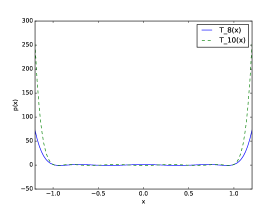
Figure 1: Two Chebyshev polynomials

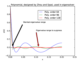
Figure 2: Polynomials from Zhou and Saad zhou2007chebyshev

To speed up the computation of the eigenvalues we are experimenting with polynomial acceleration Neff:2001zr ; Morningstar:2011ka ; Shintani:2014vja A polynomial of the matrix ($p(x)$)

$$p(D_{eo}D_{eo}^{\dagger})$$ (13)

is used in the eigensolver. The idea is to suppress the unwanted part of the eigenvalue spectrum and to spread out the required part of the spectrum. Chebyshev polynomials are a popular choice. They are of order 1 between -1 and 1, but grow rapidly outside this region. In the simplest scheme, the unwanted eigenvalues are mapped to lie between -1 and 1. See the Chebyshev polynomials in figure 2. Sorensen and Yang sorensen1997accelerating have investigated using polynomial approximations to step functions in the eigensolver, but found that the use of Chebyshev polynomials gave superior results to other polynomials they tested.

We have tested a polynomial proposed and investigated by Zhou and Saad zhou2007chebyshev . Consider a matrix $M$ with eigenvalues zhou2007chebyshev in the range $[a_{0},b]$. The polynomial is designed to suppress the eigenvalues in the range: $[a,b]$, where $a>a_{0}$. Define $e=\frac{(b-a)}{2}$ and $c=\frac{(b+a)}{2}$.

The iterative scheme for the polynomials is below

$$x_{j+1} = \frac{2}{e}(M-cI)x_{j}-x_{j-1}$$

$$x_{1} = (M-cI)x_{0}$$ (14)

Zhou and Saad zhou2007chebyshev introduced a modification to the above iterative scheme. They introduce a scaling factor $\rho_{j}=C_{j}(\frac{2}{e}(a_{0}-cI))$, so that the eigenvalues in the range $[a_{0},a]$ are mapped close to 1, and the eigenvalues in the range $[a,b]$ are mapped close to 0. In figure 2, we plot polynomials of different orders suggested by Zhou and Saad zhou2007chebyshev for target eigenvalues in the range 0.0 to 0,01.

3 Results from numerical experiments

The goal is to solve the linear equations

$$M\underline{x}=\underline{b}$$ (15)

for $\underline{x}$, given $\underline{b}$ and the fermion matrix $M$. The conjugate gradient algorithm reduces the norm of the residual ($r_{i}=M\underline{x_{i}}-\underline{b}$) at every iteration, and hence finds $\underline{x}$.

We have investigated the performance of the eigensolver and the deflated inverter using ($n_{f}$ = 2+1+1) HISQ ensembles generated by the MILC collaboration Bazavov:2010ru ; Bazavov:2012xda . Three ensembles, with lattice spacing of $a\sim 0.15$fm, were investigated. The volumes and pion masses of the three ensembles are: $16^{3}\times 48$ and $m_{\pi}\sim$ 310 MeV; $24^{3}\times 48$ and $m_{\pi}\sim$ 220 MeV; and $32^{3}\times 48$ and $m_{\pi}\sim$ 134 MeV.

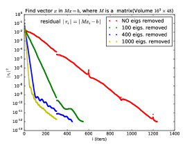
Figure 3: Square of the residual as a function of iteration with a number of eigenvalues projected out.

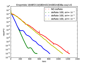
Figure 4: Square of the residual as a function of iteration with a 100 eigenvalues projected out. The eigenvalues are determined with different accuracies.

Figure 4 shows the square of the residual of the CG inverter as a function of the number of iterations as the number of deflated low eigenmodes is varied. As expected, deflation reduces the number of iterations required to get to a given residual. Progress stops when the residual reaches a value comparable the accuracy of the eigenmodes. Figure 4 shows the residual as a function of iteration when 100 eigenmodes are deflated. The eigenmodes are determined with varying accuracy using the PRIMME eigensolver.

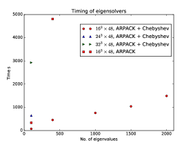
Figure 5: Preliminary timings for eigensolvers on 64 cores for the ARPACK eigensolver.

An important issue is the performance of the eigensolver, because it determines the setup cost for exact deflation. The timings for the ARPACK eigensolvers are plotted in figure 5. We are still tuning the Jacobi-Davidson algorithm in the PRIMME library. For example, the paper sorensen1997accelerating uses polynomial acceleration with a Davidson algorithm for a nonlattice QCD application. We did not optimize the polynomials used in the acceleration procedure. We stopped tuning the parameters of the algorithm once we obtained residuals around $10^{-14}$ with polynomial acceleration, so a further reduction of time can probably be made.

Figure 5 shows the preliminary time of determining different numbers of eigenmodes with different algorithms. The tests were run on 64 nodes (Intel Sandy-Bridge cores). The figure shows the dramatic speed up of the eigensolver when polynomial acceleration is used. We are still tuning the various polynomials used and the performance of the algorithm in the ARPACK library. The figure also shows the increase in time to compute the eigenvalues required as the volume is increased from $16^{3}\times 48$ to $32^{3}\times 48$.

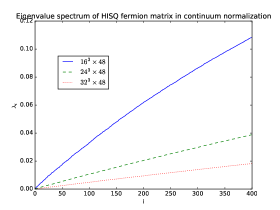
Figure 6: Eigenvalue spectrum on the three ensembles 

The performance of the eigensolver depends on the separation between the eigenvalues, so it is useful to study the first O(1000) eigenvalues. The majority (apart from Catillo:2017qbz .) of the studies of the eigenvalues of the lattice Dirac operators has focused on the smallest eigenvalues, because these are related to topology.

In figure 6 we plot the the eigenvalues of $D_{eo}$ (computed from the square root of the eigenvalues of $D_{eo}D_{eo}^{\dagger}$) on the three volumes. The magnitude of the eigenvalues is approximately linear against the mode number. A simple scaling of the bulk eigenvalues with $\frac{1}{V}$ for the space-time volume $V$ doesn’t map the eigenvalues onto a universal curve, so more study is required of the volume dependence. A log scale on the y-axis would help to reveal the potential zero modes. Follana et al. Follana:2005km argued that the near-zero topological eigenmodes scale differently with volume than the bulk eigenmodes.

4 Conclusions

There are many places in lattice QCD calculations where the computation of thousands of eigenmodes are required, either in speeding up the calculation of propagators, or in the design of better measurement techniques. Our experience has been that a lot of tuning is required to get even reasonable performance from an eigensolver. It would be useful to have a better understanding trefethen1997numerical of how to construct improved polynomials to use with an eigensolver.

We thank Carsten Urbach, Christoph Lehner, and Abdou Abdel-Rehim for discussions. This work used the Darwin Data Analytic system at the University of Cambridge, operated by the University of Cambridge High Performance Computing Service on behalf of the STFC DiRAC HPC Facility (www.dirac.ac.uk). This equipment was funded by a BIS National E-infrastructure capital grant (ST/K001590/1), STFC capital grants ST/H008861/1 and ST/H00887X/1, and DiRAC Operations grant ST/K00333X/1. DiRAC is part of the National E-Infrastructure.

References

- (1) B. Chakraborty, C.T.H. Davies, P.G. de Oliviera, J. Koponen, G.P. Lepage (2016), 1601.03071
- (2) E. Shintani, R. Arthur, T. Blum, T. Izubuchi, C. Jung, C. Lehner, Phys. Rev. D91, 114511 (2015), 1402.0244
- (3) C. Lehner, Multi-grid Lanczos, in Proceedings, 35th International Symposium on Lattice Field Theory (Lattice2017): Granada, Spain, to appear in EPJ Web Conf., 1710.01000
- (4) R. Babich, J. Brannick, R.C. Brower, M.A. Clark, T.A. Manteuffel, S.F. McCormick, J.C. Osborn, C. Rebbi, Phys. Rev. Lett. 105, 201602 (2010), 1005.3043
- (5) A. Frommer, K. Kahl, S. Krieg, B. Leder, M. Rottmann, SIAM J. Sci. Comput. 36, A1581 (2014), 1303.1377
- (6) A. Frommer, K. Kahl, S. Krieg, B. Leder, M. Rottmann (2013), 1307.6101
- (7) P.A. Boyle (2014), 1402.2585
- (8) J. Frank, C. Vuik, SIAM Journal on Scientific Computing 23, 442 (2001)
- (9) Y. Saad, M. Yeung, J. Erhel, F. Guyomarc’h, SIAM Journal on Scientific Computing 21, 1909 (2000)
- (10) R.B. Morgan, W. Wilcox (2004), math-ph/0405053
- (11) D. Darnell, R.B. Morgan, W. Wilcox, Linear Algebra Appl. 429, 2415 (2008), 0707.0502
- (12) A.M. Abdel-Rehim, R.B. Morgan, D.A. Nicely, W. Wilcox, SIAM J. Sci. Statist. Comput. 32, 129 (2008), 0806.3477
- (13) W.M. Wilcox, PoS LAT2007, 025 (2007), 0710.1813
- (14) A. Li et al. (xQCD), Phys. Rev. D82, 114501 (2010), 1005.5424
- (15) M. Luscher, JHEP 07, 081 (2007), 0706.2298
- (16) M. Luscher, JHEP 12, 011 (2007), 0710.5417
- (17) L. Trefethen, D. Bau, Numerical Linear Algebra, Other Titles in Applied Mathematics (Society for Industrial and Applied Mathematics (SIAM, 3600 Market Street, Floor 6, Philadelphia, PA 19104), 1997), ISBN 9780898719574, https://books.google.co.uk/books?id=JaPtxOytY7kC
- (18) A. Stathopoulos, K. Orginos, SIAM J. Sci. Comput. 32, 439 (2010), 0707.0131
- (19) N. Cundy, W. Lee, Comput. Phys. Commun. 203, 1 (2016), 1501.01855
- (20) B. Jegerlehner (1996), hep-lat/9612014
- (21) T. Kalkreuter, Phys. Rev. D51, 1305 (1995), hep-lat/9408013
- (22) E.S. Weinberg, R.C. Brower, K. Clark, A. Strelchenko, PoS LATTICE2016, 273 (2017)
- (23) E. Weinberg, Update on a Staggered Multigrid Algorithm in Four Dimensions, in Proceedings, 35th International Symposium on Lattice Field Theory (Lattice2017): Granada, Spain, to appear in EPJ Web Conf., 1710.01000
- (24) H. Neff, N. Eicker, T. Lippert, J.W. Negele, K. Schilling, Phys. Rev. D64, 114509 (2001), hep-lat/0106016
- (25) T.A. DeGrand, S. Schaefer, Comput. Phys. Commun. 159, 185 (2004), hep-lat/0401011
- (26) J. Foley, K. Jimmy Juge, A. O’Cais, M. Peardon, S.M. Ryan, J.I. Skullerud, Comput. Phys. Commun. 172, 145 (2005), hep-lat/0505023
- (27) G.S. Bali, S. Collins, A. Schafer, Comput. Phys. Commun. 181, 1570 (2010), 0910.3970
- (28) G. Bali, S. Collins, A. Frommer, K. Kahl, I. Kanamori, B. MÃller, M. Rottmann, J. Simeth, PoS LATTICE2015, 350 (2015), 1509.06865
- (29) A. Abdel-Rehim, C. Alexandrou, M. Constantinou, J. Finkenrath, K. Hadjiyiannakou, K. Jansen, C. Kallidonis, G. Koutsou, A.V. AvilÃs-Casco, J. Volmer, PoS LATTICE2016, 155 (2016), 1611.03802
- (30) M. CÃ, L. Giusti, S. Schaefer, Phys. Rev. D93, 094507 (2016), 1601.04587
- (31) E. Follana, Q. Mason, C. Davies, K. Hornbostel, G.P. Lepage, J. Shigemitsu, H. Trottier, K. Wong (HPQCD, UKQCD), Phys. Rev. D75, 054502 (2007), hep-lat/0610092
- (32) T. Kalkreuter, H. Simma, Comput. Phys. Commun. 93, 33 (1996), hep-lat/9507023
- (33) A. Stathopoulos, J.R. McCombs, ACM Transactions on Mathematical Software (TOMS) 37, 21 (2010)
- (34) R.B. Lehoucq, D.C. Sorensen, C. Yang, ARPACK users’ guide: solution of large-scale eigenvalue problems with implicitly restarted Arnoldi methods, Vol. 6 (Siam, 1998)
- (35) T. Kalkreuter, Comput. Phys. Commun. 95, 1 (1996), hep-lat/9509071
- (36) Z. Bai, J. Demmel, J. Dongarra, A. Ruhe, H. van der Vorst, Templates for the Solution of Algebraic Eigenvalue Problems: A Practical Guide, SIAM e-books (Society for Industrial and Applied Mathematics (SIAM, 3600 Market Street, Floor 6, Philadelphia, PA 19104), 2000), ISBN 9780898719581, https://books.google.co.uk/books?id=TOwacg5-QNoC
- (37) Y. Zhou, Y. Saad, SIAM Journal on Matrix Analysis and Applications 29, 954 (2007)
- (38) C. Morningstar, J. Bulava, J. Foley, K.J. Juge, D. Lenkner, M. Peardon, C.H. Wong, Phys. Rev. D83, 114505 (2011), 1104.3870
- (39) D. Sorensen, C. Yang, TR97-29, Dept. of Computational and Applied Mathematics, Rice University, Houston, TX (1997)
- (40) A. Bazavov et al. (MILC), Phys. Rev. D82, 074501 (2010), 1004.0342
- (41) A. Bazavov et al. (MILC), Phys. Rev. D87, 054505 (2013), 1212.4768
- (42) M. Catillo, L.Ya. Glozman (2017), 1709.01886
- (43) E. Follana, A. Hart, C.T.H. Davies, Q. Mason (HPQCD, UKQCD), Phys. Rev. D72, 054501 (2005), hep-lat/0507011