Entropy of higher-dimensional charged de Sitter black holes and phase transition

Abstract

From a new perspective, we discuss the thermodynamic entropy of $n+2$-dimensional Reissner-Nordström-de Sitter(RNdS) black hole and analyze the phase transition of the effective thermodynamic system. Considering the correlations between the black hole event horizon and the cosmological horizon, we conjecture that the total entropy of the RNdS black hole should contain an extra term besides the sum of the entropies of the two horizons. In the lukewarm case, the effective temperature of the RNdS black hole is the same as that of the black hole horizon and the cosmological horizon. Under this condition, we obtain the extra contribution to the total entropy. With the corrected entropy, we derive other effective thermodynamic quantities and analyze the phase transition of the RNdS black hole in analogy to the usual thermodynamic system.

I Introduction

Black holes are exotic objects in the theory of classical and quantum gravity. Even more surprising is their connection with the laws of standard thermodynamics. Since black hole thermodynamics is expected to play a role in any meaningful theory of gravity, therefore it will be a natural question to ask whether the thermodynamic properties of black holes are modified if higher dimensional corrections are incorporated in the Einstein-Hilbert action. One can expect a similar situation to appear in an effective theory of quantum gravity, such as string theory.

Black holes in different various dimensional sapcetime with different geometric properties have been drawing many interests. Many physical properties of black holes are related to its thermodynamic properties, such as entropy, Hawking radiation. Recently, the idea of including the variation of the cosmological constant $\Lambda$ in the first law of black hole thermodynamics has attained increasing attention Kastor-2009 ; Kubiznak:2012 ; Dolan:2011 ; Gunasekaran ; Banerjee:2011raa ; Cai:2013 ; Zhao:2013 ; Ma.2014 ; Dolan.2014 ; Ma.2014b ; Ma.2015 ; Ma.2015b ; ZhaoHH.2015 ; BEP:2015 ; Dehghani ; YXL:2016 ; Hendi:2016 ; Panahiyan:2016 ; Chabab:2016 ; Miao:2016 ; Sadeghi:2016 ; Meng:2016 ; Poshteh:2017 ; BEP:2017 ; Ma:2017 . Comparing the thermodynamic quantities in AdS black holes with those of conventional thermodynamic system, the P-V criticalities of these black holes have been extensively studied. It is shown that the phase structure, critical exponent and Clapeyron equation of the AdS black holes are similar to those of a van der Waals liquid/gas system.

As is well known, de Sitter black holes can have both the black hole event horizon and the cosmological horizon. Both the horizons can radiate, however their temperatures are different generally. Therefore, the whole de Sitter black hole system is thermodynamically unstable. We also know that the two horizons both satisfy the first law of thermodynamics and the corresponding entropies both satisfy the area lawCai:2002 ; Sekiwa ; Urano . In recent years, the studies on the thermodynamic properties of de Sitter space have aroused wide attentionCai:2002 ; Sekiwa ; Urano ; Gombero:2003 ; Mann:2005 ; Padmanabhan:2007 ; Bhattacharya ; Katsuragawa ; MAA1 ; MAA2 ; Hajian ; Kubiznak ; McInerney ; Li-2016 . In the early inflation epoch, the universe is a quasi-de Sitter spacetime. If the cosmological constant is the dark energy, our universe will evolve to a new de Sitter phase.

Because the two horizons are expressed by the same parameters: the mass M, electric charge Q and the cosmological constant $\Lambda$, they should be dependent each other. Taking into account of the correlations between the two horizons is very important for the description of the thermodynamic properties of de Sitter black holes. Previous works, such as Refs.Mellor ; Romans ; Cai:1998 ; BPD:2013 ; ZR:2014 ; ZLC:2014 ; ZHH ; MMS:2014 ; Brenna ; Poshteh2 ; Ma ; Guo2 ; ZLC ; Guo1 ; MYQ , considered that the entropy of the de Sitter black holes is the sum of the black hole entropy and the entropy of the cosmological horizon. Based on this consideration, the effective thermodynamic quantities and phase transition are analyzed. It shows that de Sitter black holes have the similar critical behaviors to those of black holes in anti-de Sitter space. However, considering the correlation or entanglement between the event horizon and the cosmological horizon, the total entropy of the charged black hole in de Sitter space is no longer simply $S=S_{+}+S_{c}$, but should include an extra term from the contribution of the correlations of the two horizonsZLC:2016 ; LHF:2017 .

In this paper, we study the $(n+2)$-dimensional Reissner-Nordström-dS black hole by considering the correlation of the black hole horizon and the cosmological horizon. In the Sec.II, we review the various thermodynamic quantities on the both horizons and give the condition under which the temperatures of the two horizons are equal. In Sec. III, we derive the effective thermodynamic quantities and propose the expression of the whole entropy. In Sec. IV, the phase transition of the higher-dimensional RN-dS black hole is studied according to the Ehrenfest’s equations. At last, we will give the conclusions. (we use the units $\hbar=k_{B}=c=1)$.

II Lukewarm $(n+2)$-dimensional Reissner-Nordstrom solutions in de Sitter space

The line element of the $(n+2)$-dimensional RNdS black hole is given byCai:2002

$$ds^{2}=-f(r)dt^{2}+f^{-1}(r)dr^{2}+r^{2}d\Omega_{n}^{2},$$ (1)

where

$$f(r)=1-\frac{\omega_{n}M}{r^{n-1}}+\frac{n\omega_{n}^{2}Q^{2}}{8(n-1)r^{2n-2}}-\frac{r^{2}}{l^{2}},\quad\omega_{n}=\frac{16\pi G}{nVol(S^{n})}.$$ (2)

Here $G$ is the gravitational constant in $(n+2)$ dimensions, $l$ is the curvature radius of dS space, $Vol(S^{n})$ denotes the volume of a unit $n$-sphere $d\Omega_{n}^{2}$, $M$ is an integration constant and $Q$ is the electric/magnetic charge of Maxwell field. For general $M$ and $Q$, the equation $f(r)=0$ may have four real roots. Three of them are real: the largest one is the cosmological horizon $r_{c}$, the smallest is the inner (Cauchy) horizon of black hole, the middle one is the event horizon $r_{+}$ of black hole. Some thermodynamic quantities associated with the cosmological horizon are

$$T_{c} = \frac{1}{4\pi r_{c}}\left[{-(n-1)+(n+1)\frac{r_{c}^{2}}{l^{2}}+\frac{n\omega_{n}^{2}Q^{2}}{8r_{c}^{2n-2}}}\right],$$ (3)

$$S_{c} = \frac{r_{c}^{n}Vol(S^{n})}{4G},$$ (4)

$$\Phi_{c} = \frac{n}{4(n-1)}\frac{\omega_{n}Q}{r_{c}^{n-1}},$$ (5)

where $\Phi_{c}$ is the chemical potential conjugate to the charge $Q$. The first law of thermodynamics of the cosmological horizon is BPD:2013

$$dM=T_{c}dS_{c}+V_{c}dP+\Phi_{c}dQ,$$ (6)

$$P=-\frac{n(n+1)}{16\pi l^{2}},\quad V_{c}=\frac{Vol(S^{n})}{(n+1)}r_{c}^{n+1}.$$ (7)

For the black hole horizon, associated thermodynamic quantities are

$$T_{+} = \frac{1}{4\pi r_{+}}\left[{(n-1)-(n+1)\frac{r_{+}^{2}}{l^{2}}-\frac{n\omega_{n}^{2}Q^{2}}{8r_{+}^{2n-2}}}\right],$$ (8)

$$S_{+} = \frac{r_{+}^{n}Vol(S^{n})}{4G},$$ (9)

$$\Phi_{+} = \frac{n}{4(n-1)}\frac{\omega_{n}Q}{r_{+}^{n-1}}.$$ (10)

The first law of thermodynamics of the black hole horizon isBPD:2013

$$dM=T_{+}dS_{+}+V_{+}dP+\Phi_{+}dQ,$$ (11)

$$V_{+}=\frac{Vol(S^{n})}{(n+1)}r_{+}^{n+1}.$$ (12)

In the following, we find the “lukewarm” $(n+2)$-dimensional RN solutions which realize this state of affairs, that is, describing an outer black hole horizon at radius $r_{+}$ and a de Sitter edge at radius $r_{c}$, with the same Hawking temperature at $r_{+}$ and $r_{c}$. In terms of the metric function $f(r)$, the algebraic problem is Cai:1998 ; Romans ; Mellor

$$f(r_{c})=f(r_{+})=0;\quad f^{\prime}(r_{c})=\pm f^{\prime}(r_{+}),$$ (13)

where the minus sign is appropriate, since there should be no roots of $f(r)$ between $r_{+}$ and $r_{c}$.

According to $f(r_{+})=f(r_{c})=0$, one can derive

$$\frac{1}{l^{2}}=\frac{r_{c}^{n-1}-r_{+}^{n-1}}{r_{c}^{n+1}-r_{+}^{n+1}}\left[{1-\frac{A}{(n-1)}}\right],$$ (14)

and

$$\omega_{n}M=r_{c}^{n-1}x^{n-1}\frac{1-x^{2}}{1-x^{n+1}}+\frac{n\omega_{n}^{2}Q^{2}}{8(n-1)r_{c}^{n-1}x^{n-1}}\frac{1-x^{2n}}{1-x^{n+1}}.$$ (15)

where we have set $\frac{n\omega_{n}^{2}Q^{2}}{8(r_{c}r_{+})^{n-1}}=\frac{n\omega_{n}^{2}Q^{2}}{8r_{c}^{2n-2}x^{n-1}}=A$ and $x=r_{+}/r_{c}$.

From $T_{+}=T_{c}$, we can get

$$\frac{r_{c}^{n-1}-r_{+}^{n-1}}{r_{c}^{n+1}-r_{+}^{n+1}}-\frac{(n-1)}{(n+1)r_{c}r_{+}}=\frac{n\omega_{n}^{2}Q^{2}}{8}F(r_{+},r_{c},n).$$ (16)

where

$$F(r_{+},r_{c},n)=\frac{(r_{c}^{n-1}-r_{+}^{n-1})}{(n-1)r_{c}^{n-1}r_{+}^{n-1}(r_{c}^{n+1}-r_{+}^{n+1})}-\frac{r_{c}^{2n-1}+r_{+}^{2n-1}}{(n+1)r_{+}^{2n-1}r_{c}^{2n-1}(r_{c}+r_{+})}.$$ (17)

Substituting Eqs. (14) and (15) into Eqs. (3) and (8), the lukewarm temperature $T_{c+}$ is

$$T_{c+} = \frac{T_{+}+T_{c}}{2}$$ (18)

$$= \frac{(n-1)(1-x)}{4\pi r_{c}x}-\frac{(1-x^{2n})}{4\pi r_{c}x^{2n-1}(1+x)r_{c}^{2n}F(r_{c},x,n)}\left[{\frac{1-x^{n-1}}{1-x^{n+1}}-\frac{(n-1)}{(n+1)x}}\right],$$

where

$$F(r_{c},x,n)=\frac{(1-x^{n-1})}{(n-1)r_{c}^{n}x^{n-1}(1-x^{n+1})}-\frac{1+x^{2n-1}}{(n+1)r_{c}^{2n}x^{2n-1}(1+x)}.$$ (19)

When the cosmological constant satisfies Eq.(14), and the electric charge Q satisfies Eq.(16), the temperatures of the two horizons are equal, which is given in Eq.(18).

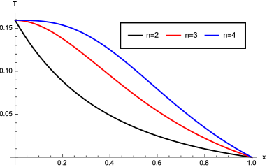
Figure 1: The temperature of lukewarm black hole as function of $x$ for different spacetime dimensions. We have set $r_{c}=1$.

As is depicted in Fig.1, in the lukewarm case, the temperature of the horizons increases with the dimension of spacetime and monotonically decreases with the increase of $x$. This means that the closer the two horizons are, the lower of their temperature will be.

III Entropy of the $(n+2)$-dimensional RNdS black hole

The thermodynamic quantities of $(n+2)$-dimensional RNdS black hole satisfyZR:2014 ; ZLC:2014

$$dM=T_{eff}dS-P_{eff}dV+\Phi_{eff}dQ,$$ (20)

where the thermodynamic volume is McInerney ; BPD:2013 ; Brenna

$$V=V_{c}-V_{+}=\frac{Vol(S^{n})}{(n+1)}(r_{c}^{n+1}-r_{b}^{n+1})=\frac{Vol(S^{n})}{(n+1)}r_{c}^{n+1}(1-x^{n+1}).$$ (21)

The effective temperature, the effective pressure and the effective electric potential are respectively

$$T_{eff}=\left({\frac{\partial M}{\partial S}}\right)_{Q,V}=\frac{\left({\frac{\partial M}{\partial x}}\right)_{r_{c}}\left({\frac{\partial V}{\partial r_{c}}}\right)_{x}-\left({\frac{\partial V}{\partial x}}\right)_{r_{c}}\left({\frac{\partial M}{\partial r_{c}}}\right)_{x}}{\left({\frac{\partial S}{\partial x}}\right)_{r_{c}}\left({\frac{\partial V}{\partial r_{c}}}\right)_{x}-\left({\frac{\partial V}{\partial x}}\right)_{r_{c}}\left({\frac{\partial S}{\partial r_{c}}}\right)_{x}},$$ (22)

$$P_{eff}=-\left({\frac{\partial M}{\partial V}}\right)_{Q,S}=-\frac{\left({\frac{\partial M}{\partial x}}\right)_{r_{c}}\left({\frac{\partial S}{\partial r_{c}}}\right)_{x}-\left({\frac{\partial S}{\partial x}}\right)_{r_{c}}\left({\frac{\partial M}{\partial r_{c}}}\right)_{x}}{\left({\frac{\partial V}{\partial x}}\right)_{r_{c}}\left({\frac{\partial S}{\partial r_{c}}}\right)_{x}-\left({\frac{\partial S}{\partial x}}\right)_{r_{c}}\left({\frac{\partial V}{\partial r_{c}}}\right)_{x}},$$ (23)

$$\Phi_{eff}=\left({\frac{\partial M}{\partial Q}}\right)_{S,V}.$$ (24)

For a system composed of two subsystems, the total entropy should be the simple sum of the entropies of the two subsystems if there is no interactions between them. When correlation exists between the two subsystems, the total entropy should contain an extra contribution coming from the correlations between the two subsystems. Considering the correlation between the two horizons, we conjecture that the entropy of the $(n+2)$-dimensional RNdS black hole should take the form of

$$S=\frac{Vol(S^{n})}{4G}r_{c}^{n}(1+x^{n}+f(x)),$$ (25)

where the undefined function $f(x)$ represents the extra contribution from the correlations of the two horizons. Next we try to determine the concrete form of $f(x)$.

Substituting Eqs. (15), (21) and (25) into Eq. (22), we can get

$$T_{eff}=\frac{4G}{Vol(S^{n})r_{c}^{n-1}}\frac{\frac{1}{r_{c}}\left({\frac{\partial M}{\partial x}}\right)_{r_{c}}\left({1-x^{n+1}}\right)+\left({\frac{\partial M}{\partial r_{c}}}\right)_{x}x^{n}}{(nx^{n-1}+f^{\prime}(x))(1-x^{n+1})+nx^{n}(1+x^{n}+f(x))}.$$ (26)

From Eq.(15), we can derive

$$\left({\frac{\partial M}{\partial r_{c}}}\right)_{x}=(n-1)\frac{r_{c}^{n-2}x^{n-1}}{\omega_{n}}\left({\frac{1-x^{2}}{1-x^{n+1}}}\right)\frac{n\omega_{n}Q^{2}(1-x^{2n})}{8r_{c}^{n}x^{n-1}(1-x^{n+1})},$$ (27)

and

$$\left({\frac{\partial M}{\partial x}}\right)_{r_{c}}=\frac{r_{c}^{n-1}}{\omega_{n}}\frac{(n-1)x^{n-2}-(n+1)x^{n}+2x^{2n-1}}{(1-x^{n+1})^{2}}+\frac{n\omega_{n}Q^{2}(2nx^{n+1}-(n-1)-(n+1)x^{2n})}{8(n-1)r_{c}^{n-1}x^{n}(1-x^{n+1})^{2}}.$$ (28)

When the temperatures of the two horizons are the same, the charge $Q$ satisfies Eq.(16). Thus, we can derive the effective temperature $T_{eff}$ in the lukewarm case:

$$T_{eff}=\frac{n}{4\pi r_{c}}\frac{A+B}{(nx^{n-1}+f^{\prime}(x))(1-x^{n+1})+nx^{n}(1+x^{n}+f(x))},$$ (29)

where

$$A=\frac{(n-1)x^{n-2}-(n+1)x^{n}+2x^{2n-1}}{(1-x^{n+1})}+\frac{2nx^{n+1}-(n-1)-(n+1)x^{2n}}{(n-1)x^{n}(1-x^{n+1})F_{0}(r_{c},x,n)}\left({\frac{(1-x^{n-1})}{-x^{n+1})}-\frac{(n-1)}{(n+1)x}}\right),$$

$$B=(n-1)x^{2n-1}\left({\frac{1-x^{2}}{1-x^{n+1}}}\right)\frac{x(1-x^{2n})}{(1-x^{n+1})F_{0}(r_{c},x,n)}\left({\frac{(1-x^{n-1})}{-x^{n+1})}-\frac{(n-1)}{(n+1)x}}\right),$$

with

$$F_{0}(r_{c},x,n)=\frac{(1-x^{n-1})}{(n-1)x^{n-1}(1-x^{n+1})}-\frac{1+x^{2n-1}}{(n+1)x^{2n-1}(1+x)}.$$

When the two horizons have the same temperature, we think the effective temperature of the system should have the same value, namely

$$T_{eff}=T_{c}=T_{+}=T_{c+}.$$ (30)

According to Eqs. (18) and (29), we derive the equations about $f(x)$:

$$f^{\prime}(x)-\frac{nx^{n}f(x)}{x^{n+1}-1}=\frac{nx^{n}\left(2x^{n+1}+x^{n}-1\right)}{\left(x^{n+1}-1\right)^{2}}.$$ (31)

For $n=2,~{}n=3,~{}n=4$, the field equations about $f(x)$ are respectively :

$$f^{\prime}(x)+\frac{2x^{2}f(x)}{1-x^{3}} = \frac{2x^{2}\left(2x^{3}+x^{2}-1\right)}{\left(1-x^{3}\right)^{2}},$$ (32)

$$f^{\prime}(x)+\frac{3x^{3}f(x)}{1-x^{4}} = \frac{3x^{3}\left(2x^{4}+x^{3}-1\right)}{\left(1-x^{4}\right)^{2}},$$ (33)

$$f^{\prime}(x)+\frac{4x^{4}f(x)}{1-x^{5}} = \frac{4x^{4}\left(2x^{5}+x^{4}-1\right)}{\left(1-x^{5}\right)^{2}}.$$ (34)

And the solutions for these equations are respectively:

$$f(x) = \frac{8}{5}\left(1-x^{3}\right)^{2/3}-\frac{2\left(x^{5}+5x^{3}-4\right)}{5\left(x^{3}-1\right)},$$ (35)

$$f(x) = \frac{11}{7}\left(1-x^{4}\right)^{3/4}+\frac{-3x^{6}+3x^{5}-3x^{4}-11x^{3}+11x^{2}-11x+11}{7\left(x^{3}-x^{2}+x-1\right)},$$ (36)

$$f(x) = \frac{14}{9}\left(1-x^{5}\right)^{4/5}+\frac{2\left(-2x^{9}-9x^{5}+7\right)}{9\left(x^{5}-1\right)},$$ (37)

where we have taken the boundary condition $f(0)=0$, because $x=0$ means the absence of the black hole horizon and thus no correlation between the black hole horizon and the cosmological horizon.

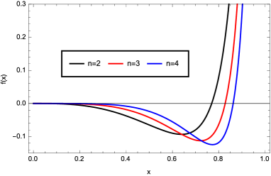
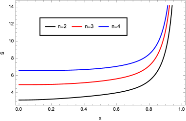
Figure 2: The left panel depicts $f(x)$ as functions of $x$ for $n+2$-dimensional RNdS black hole. The right panel depicts the whole entropy $S$ of the RNdS black hole in different dimensions. We have set $r_{c}=1$.

As is shown in Fig.2, the value of $f(x)$ does not vary monotonically. It first decreases as the $x$ increases, at some point it reaches a minimum and then begins to increase to the infinity at $x=1$. The entropy $S$ increases with the spacetime deimension $n$ and diverges as $x\rightarrow 1$. We also depict the effective temperature $T_{eff}$ in Fig.3, from which we can see that $T_{eff}$ tends to zero as $x\to 1$, namely the charged Nariai limit. Although this result does not agree with that of Bousso and HawkingBousso , it is consistent with the entropy. Besides, the temperature has a maximum. The maximum of the temperature is dependent on the values of $n$ and $Q$. For larger $n$, the maximum lies at bigger $x$. And for larger $Q$, the maximum will be smaller.

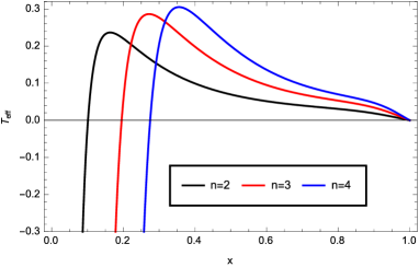
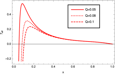
Figure 3: The effective temperature as functions of $x$. The left panel depicts $T_{eff}$ at fixed $Q=0.05$. The right panel depicts depicts $T_{eff}$ at fixed $n=3$. We have set $r_{c}=1$.

IV Phase transition in RN-dS black hole spacetime

In analogy to the van der Waals liquid/gas system, one can analyze the black hole thermodynamic system. One can derive the critical exponent, Ehrenfest’s equations. However, the de Sitter black hole cannot be in thermodynamically equilibrium state in the usual sense due to the different temperatures on the two horizons. From Eq.(3.6), the entropy of dS black holes should contain an extra term $f(x)$. This result is obtained from the first law of thermodynamics, which is the universal for usual thermodynamic system. Thus, the entropy of the dS black hole we derived is closer to that of usual thermodynamic system.

When $n=2$, the effective potential is

$$\Phi_{eff}=\frac{Q(1-x^{4})}{r_{c}x(1-x^{3})},$$ (38)

We can adjust the $T_{eff}$ as the function $\Phi_{eff}$, but not $Q$. So it is

$$T_{eff}=\frac{\Phi^{2}\left(x^{2}+x+1\right)^{2}\left[x^{3}\left(x^{4}-3x+3\right)-1\right]-x^{2}(x+1)^{2}\left(x^{2}+1\right)^{2}\left[x^{2}\left(x^{3}-3x+3\right)-1\right]}{4\pi x^{3}\left(x^{3}+x^{2}+x+1\right)^{2}\left(x^{4}+1\right)r_{c}}.$$ (39)

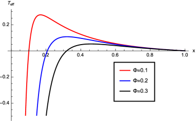
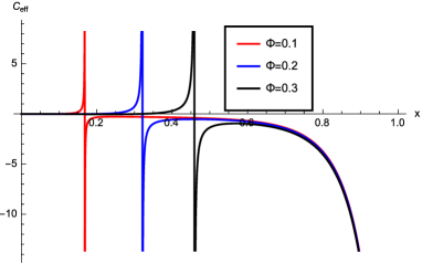
Figure 4: The effective temperature and the effective heat capacity as functions of $x$ for different $\Phi_{eff}=0.1,~{}0.2,~{}0.3$ with fixed $n=2$. We have set $r_{c}=1$.

The effective heat capacity can be defined as

$$C_{\Phi_{eff}}=T_{eff}\left({\frac{\partial S}{\partial T_{eff}}}\right)_{\Phi_{eff}}.$$ (40)

In Fig.4, we depict the effective temperature and the heat capacity at the fixed $\Phi_{eff}$ ensemble. It is shown that the heat capacity will diverge at the point where the effective temperature takes maximum. As the value of $\Phi_{eff}$ increases, the position of the divergent point moves right. Only on the left-hand side of that point, the heat capacity is positive. This means that the effective thermodynamic system is thermodynamically stable when the two horizons have a long way off.

The analog of volume expansion coefficient and analog of isothermal compressibility are given by

$$\alpha=\frac{1}{Q}\left({\frac{\partial Q}{\partial T_{eff}}}\right)_{\Phi_{eff}},\kappa_{T_{eff}}=-\frac{1}{Q}\left({\frac{\partial Q}{\partial\Phi_{eff}}}\right)_{T_{eff}}.$$ (41)

They have the similar behaviors to that of the effective heat capacity.

We now exploit Ehrenfest’s scheme in order to understand the nature of the phase transition. Ehrenfest’s scheme basically consists of a pair of equations known as Ehrenfest’s equations of first and second kind. For a standard thermodynamic system these equations may be written as

$$-\left({\frac{\partial\Phi_{eff}}{\partial T_{eff}}}\right)_{S}=\frac{C_{\Phi_{eff}}^{2}-C_{\Phi_{eff}}^{1}}{T_{eff}V(\alpha^{2}-\alpha^{1})}=\frac{\Delta C_{\Phi_{eff}}}{T_{eff}V\Delta\alpha},$$ (42)

$$-\left({\frac{\partial\Phi_{eff}}{\partial T_{eff}}}\right)_{V}=\frac{\alpha^{2}-\alpha^{1}}{\kappa^{2}-\kappa^{1}}=\frac{\Delta\alpha}{\Delta\kappa}.$$ (43)

The subscript 1 and 2 represent phase 1 and 2 respectively. The new variables $\alpha$ and $\kappa_{T_{eff}}$ correspond to the volume expansivity and isothermal compressibility in statistical thermodynamics.

From the Maxwell’s relations,

$$\left({\frac{\partial Q}{\partial S}}\right)_{T_{eff}}=-\left({\frac{\partial T_{eff}}{\partial\Phi_{eff}}}\right)_{Q},\quad\left({\frac{\partial S}{\partial Q}}\right)_{\Phi_{eff}}=-\left({\frac{\partial\Phi_{eff}}{\partial T_{eff}}}\right)_{S}$$ (44)

substituting Eq.(44) into Eqs.(42) and (43), we can obtain

$$\frac{\Delta C_{\Phi_{eff}}}{T_{eff}V\Delta\alpha}=-\left({\frac{\partial S}{\partial Q}}\right)_{\Phi_{eff}}^{c},\quad\frac{\Delta\alpha}{\Delta\kappa}=-\left({\frac{\partial S}{\partial Q}}\right)_{T_{eff}}^{c}.$$ (45)

Note that the superscript “c” denotes the values of physical quantities at a critical point in our article, while we find that

$$\left({\frac{\partial S}{\partial Q}}\right)_{\Phi_{eff}}=\frac{\left({\frac{\partial S}{\partial x}}\right)_{r_{c}}\left({\frac{\partial\Phi_{eff}}{\partial r_{c}}}\right)_{x}-\left({\frac{\partial\Phi_{eff}}{\partial x}}\right)_{r_{c}}\left({\frac{\partial S}{\partial r_{c}}}\right)_{x}}{\left({\frac{\partial Q}{\partial x}}\right)_{r_{c}}\left({\frac{\partial\Phi_{eff}}{\partial r_{c}}}\right)_{x}-\left({\frac{\partial\Phi_{eff}}{\partial x}}\right)_{r_{c}}\left({\frac{\partial Q}{\partial r_{c}}}\right)_{x}},$$ (46)

$$\left({\frac{\partial S}{\partial Q}}\right)_{T_{eff}}=\frac{\left({\frac{\partial S}{\partial x}}\right)_{r_{c}}\left({\frac{\partial T_{eff}}{\partial r_{c}}}\right)_{x}-\left({\frac{\partial T_{eff}}{\partial x}}\right)_{r_{c}}\left({\frac{\partial S}{\partial r_{c}}}\right)_{x}}{\left({\frac{\partial Q}{\partial x}}\right)_{r_{c}}\left({\frac{\partial T_{eff}}{\partial r_{c}}}\right)_{x}-\left({\frac{\partial T_{eff}}{\partial x}}\right)_{r_{c}}\left({\frac{\partial Q}{\partial r_{c}}}\right)_{x}},$$ (47)

When $\left({\frac{\partial Q}{\partial x}}\right)_{r_{c}}\left({\frac{\partial T_{eff}}{\partial r_{c}}}\right)_{x}-\left({\frac{\partial T_{eff}}{\partial x}}\right)_{r_{c}}\left({\frac{\partial Q}{\partial r_{c}}}\right)_{x}\neq 0$, the critical points satisfy

$$\left({\frac{\partial T_{eff}}{\partial x}}\right)_{r_{c}}\left({\frac{\partial\Phi_{eff}}{\partial r_{c}}}\right)_{x}-\left({\frac{\partial\Phi_{eff}}{\partial x}}\right)_{r_{c}}\left({\frac{\partial T_{eff}}{\partial r_{c}}}\right)_{x}=0.$$ (48)

Substituting Eq. (48) into Eq. (46), we have

$$\left({\frac{\partial S}{\partial Q}}\right)_{\Phi_{eff}}^{c}=\left({\frac{\partial S}{\partial Q}}\right)_{T_{eff}}^{c}.$$ (49)

So far, we have proved that both the Ehrenfest equations are correct at the critical point. Utilizing Eq .(49), the Prigogine–Defay (PD) ratio ($\Pi)$can be calculated as

$$\Pi=\frac{\Delta C_{\Phi_{eff}}\Delta\kappa_{T_{eff}}}{T_{eff}^{c}V^{c}(\Delta\alpha)^{2}}=1.$$ (50)

Hence the phase transition occurring at $T_{eff}=T_{eff}^{c}$ is a second order equilibrium transition . This is true in spite of the fact that the phase transition curves are smeared and divergent near the critical point.

V Conclusions

In this paper, we first propose the condition under which the black hole horizon and the cosmological horizon have the same temperature for the RN-dS black hole. We think that the entropy of these black holes with multiple horizons is not simply the sum of the entropies of every horizon, but should contains an extra contribution from the correlations between the horizons. On the basis of this consideration, we put forward the expression of the entropy. According to the effective first law of black hole thermodynamics, we can derive the effective temperature $T_{eff}$, the effective pressure $P_{eff}$ and the effective potential $\Phi_{eff}$. In the lukewarm case, the temperatures of the two horizons are the same. We conjecture that the effective temperature also takes the same value. According to this relation, we can obtain the differential equation for $f(x)$. Considering the reasonable boundary condition: $f(0)=0$, we can solve the differential equation exactly and obtain the $f(x)$.

In section IV, we analyzed the phase transition of the RN-dS black hole. Near the critical point, the heat capacity, the expansion coefficient and the isothermal compressibility are all divergent, while at this point the entropy and the Gibbs free energy are continuous. Thus the phase transition at this point is of second order. From Fig.4, only when $x<x_{c}$ the heat capacity can be positive. This means that on the left-hand side of the divergent point, the effective thermodynamic system is locally thermodynamically stable.

We anticipate that study on the thermodynamic properties of the black holes in de Sitter space can shed light on the classical and quantum properties of de Sitter space.

VI acknowledgments

This work is supported in part by the National Natural Science Foundation of China (Grant No.11475108).

References

• (1) D.Β Kastor, S.Β Ray and J.Β Traschen, Class. Quant. Grav. 26(2009) 195011.
• (2) D. Kubiznak, R. B. Mann, JHEP 1207:033,2012.
• (3) B. P. Dolan, Class. Quant. Grav.28:125020,2011.
• (4) S. Gunasekaran, D.Kubiznak, R. B. Mann, JHEP11(2012)110.
• (5) R.Β Banerjee, S.Β K.Β Modak and D.Β Roychowdhury, JHEP 1210, 125 (2012).
• (6) R.-G. Cai, L.-M. Cao, L. Li, and R.-Q. Yang, JHEP09(2013)005.
• (7) R. Zhao, H. -H. Zhao, M. -S. Ma and L. -C. Zhang, Eur. Phys. J. C (2013), 73:2645.
• (8) M.-S. Ma, F.Β Liu and R.Β Zhao, Class. Quantum Grav. 31 (2014) 095001.
• (9) B.Β P. Dolan, A.Β Kostouki, D.Β KubizňÑk and R.Β B. Mann, Class. Quantum Grav. 31 (2014) 242001.
• (10) M.-S. Ma and R.Β Zhao, Phys. Rev. D 89 (2014) 044005.
• (11) M.-S. Ma and Y.-Q. Ma, Class. Quantum Grav.32 (2015) 035024.
• (12) M.-S. Ma and R.Β Zhao, Phys. Lett. B 751 (2015) 278–283.
• (13) H.-H. Zhao, L.-C. Zhang, M.-S. Ma and R. Zhao, Class. Quantum Grav. 32 (2015) 145007.
• (14) S. H. Hendi, S. Panahiyan and B. Eslam Panah, Prog. Theor. Exp. Phys. 2015 (2015) 103E01.
• (15) M. H. Dehghani, A. Sheykhi,and Z. Dayyani, Phys. Rev. D 93, 024022 (2016).
• (16) P. Cheng, S.-W. Wei, and Y.-X. Liu, Phys. Rev. D 94, 024025 (2016).
• (17) S. H. Hendi, R. Moradi, Z. Armanfard, M. S. Talezadeh, Eur. Phys. J. C 76 (2016) 263.
• (18) S. H. Hendi, S. Panahiyan, B. Eslam Panah, Z. Armanfard, Eur. Phys. J. C (2016) 76:396.
• (19) M. Chabab, H. El Moumnia, K. Masmar, Eur. Phys. J. C (2016) 76:304.
• (20) Y.-G. Miao, Z.-M. Xu, Eur. Phys. J. C (2016) 76:217.
• (21) J. Sadeghi,Β B. Pourhassan,Β M. Rostami, Phys. Rev. D 94, 064006 (2016).
• (22) H. Liu,Β X.-H. Meng, Mod. Phys. Lett. A 31(2016) 1650199.
• (23) Mohammad Bagher Jahani Poshteh,Β Nematollah Riazi, Gen. Relativ Gravit. (2017) 49: 64.
• (24) S. H. Hendi, R. B. Mann, S. Panahiyan, B. Eslam Panah, Phys. Rev. D 95 (2017)021501(R).
• (25) M.-S. Ma and R.-H. Wang, Phys. Rev. D 96(2017)024052.
• (26) R.-G. Cai, Nucl. Phys. B 628 (2002)375.
• (27) Y. Sekiwa, Phys. Rev. D 73(2006)084009.
• (28) M. Urano, A. Tomimatsu and H. Saida, Class. Quantum Grav.26(2009)105010.
• (29) A. Gomberoff, and C. Teitelboim, Phys. Rev. D,67, 104024(2003).
• (30) A. M. Ghezelbash and R. B. Mann, Phys. Rev. D,72, 064024, (2005).
• (31) T. Roy Choudhury and T. Padmanabhan, Gen. Rel. Grav.,39, 1789(2007).
• (32) S. Bhattacharya, A. Lahiri, Eur. Phys. J. C (2013),Β 73:2673.
• (33) T. Katsuragawa and S. Nojiri, Phys. Rev. DΒ 91, 084001 (2015).
• (34) M. Azreg-AΓ―nou, Eur. Phys. J. C (2015) 75:34.
• (35) M. Azreg-AΓ―nou, Phys. Rev. D 91,064049 (2015).
• (36) K. Hajian, Gen. Relativ Gravit. (2016),Β 48:114.
• (37) D. Kubiznak, F. Simovic, Class. Quantum Grav. 33(2016) 245001.
• (38) J. McInerney,Β G. Satishchandran,Β J. Traschen, Class. Quantum Grav. 33(2016)105007.
• (39) H.-F. Li, M.-S. Ma and Y.-Q. Ma, Mod. Phys. Lett. A 32 (2017) 1750017.
• (40) F. Mellor, and I. Moss, Class. Quantum. Grav. 6(1989) 1379.
• (41) L. J. Romans, Nucl.Phys. B383 (1992) 395.
• (42) R.-G. Cai, J. Y. Ji, K. S. Soh, Class. Quantum Grav. 15 (1998)2783.
• (43) B. P. Dolan,Β D. Kastor,Β D. Kubiznak,Β R. B. Mann, and J. Traschen, Phys. Rev. DΒ 87, 104017(2013).
• (44) R. Zhao, M. S. Ma, H. H. Zhao, and L. C. Zhang, Advances in High Energy Physics, 124854 (2014).
• (45) L. C. Zhang, M. S. Ma, H. H. Zhao, R. Zhao, Eur. Phys. J. C 2014, 74: 3052.
• (46) H.-H. Zhao, L.-C. Zhang, M.-S. Ma, and R. Zhao, Phys. Rev. D,90, 064018(2014).
• (47) M.-S. Ma, H.-H. Zhao, L.-C. Zhang, and R. Zhao, Int. Journal Modern Physics A(2014),29,14500050.
• (48) W. G. Brenna,Β R. B. Mann,Β M. Park, Phys. Rev. D 92, 044015 (2015).
• (49) Mohammad Bagher Jahani Poshteh,Β Behrouz Mirza,Β Fatemeh Oboudiat, Int. Journal Modern Physics D 24(2015)1550029.
• (50) M.-S. Ma, L.-C. Zhang, H.-H. Zhao and R. Zhao, Advances in High Energy Physics, 2015, 134815.
• (51) X.-Y. Guo, H.-F. Li, L.-C. Zhang and R. Zhao, Phys. Rev. D 91,084009(2015).
• (52) L. C. Zhang, R. Zhao, EPL,113(2016) 10008.
• (53) X.-Y. Guo, H.-F. Li, L.-C. Zhang and R. Zhao, Class. Quantum Grav. 33 (2016) 135004.
• (54) M.-S. Ma, R. Zhao, Y.-Q. Ma, Gen Relativ Gravit (2017) 49:79.
• (55) L.-C. Zhang, R. Zhao and M.-S. Ma, Phys. Lett. B 761 (2016)74.
• (56) H.-F. Li, M.-S. Ma, L.-C. Zhang and R. Zhao, Nucl. Phys. B 920 (2017) 211.
• (57) R. Bousso, S. W. Hawking, Phys. Rev. D54, 6312(1996).