Modeling Graphs Using a Mixture of Kronecker Models

Abstract

Generative models for graphs are increasingly becoming a popular tool for researchers to generate realistic approximations of graphs. While in the past, focus was on generating graphs which follow general laws, such as the power law for degree distribution, current models have the ability to learn from observed graphs and generate synthetic approximations. The primary emphasis of existing models has been to closely match different properties of a single observed graph. Such models, though stochastic, tend to generate samples which do not have significant variance in terms of the various graph properties. We argue that in many cases real graphs are sampled drawn from a graph population (e.g., networks sampled at various time points, social networks for individual schools, healthcare networks for different geographic regions, etc.). Such populations typically exhibit significant variance. However, existing models are not designed to model this variance, which could lead to issues such as overfitting. We propose a graph generative model that focuses on matching the properties of real graphs and the natural variance expected for the corresponding population. The proposed model adopts a mixture-model strategy to expand the expressiveness of Kronecker product based graph models (KPGM), while building upon the two strengths of KPGM, viz., ability to model several key properties of graphs and to scale to massive graph sizes using its elegant fractal growth based formulation. The proposed model, called x-Kronecker Product Graph Model, or xKPGM, allows scalable learning from observed graphs and generates samples that match the mean and variance of several salient graph properties. We experimentally demonstrate the capability of the proposed model to capture the inherent variability in real world graphs on a variety of publicly available graph data sets.

I Introduction

Data occurs as graphs and networks in a wide variety of applications, ranging from social sciences to biology. Graph analysis methods are required to understand the structural properties of graphs. One important class of graph analysis methods deal with finding generative mechanisms and models that generate graphs with such structural properties. A crucial application of these models is to generate synthetic graphs which “match” the structural properties of real world graphs. Given the limited availability of real world graph data, mainly because of high cost and privacy concerns, such synthetic (and anonymized) graphs are a valuable resource for researchers to understand network behavior in domains such as systems analysis (e.g., the Internet), bioinformatics, and social sciences, while allowing for anonymity and privacy [4]. Applications include understanding malware propagation in social networks [19], understanding fraud in healthcare [5], etc. Graph generative models also allow researchers to produce realistics simulations at desired scale which are vital to understand issues such as handling scalability challenges and modeling temporal evolution.

What should be the salient characteristics of such a generative model? First, it should be able to capture the properties of real-world graphs. Traditionally the focus has been on general “laws” that are expected to be obeyed by real world graphs, such as power laws for degree distributions, small diameters, communities, etc. However, to accurately represent the real world graph, matching on local graph properties such as edges, transitive triangles, etc., is important. Second, the model should be able to scale to massive graph sizes, to be applicable in domains where graphs tend to be big. Third, to allow generation (simulation) of any sized synthetic graphs, the model should be parametric and should allow learning of the parameters from one or more observed graphs.

Table I compares several existing graph generative models in terms of which of the above characteristics. Note that several models satisfy all three characteristics. However, we argue that there is an additional characteristic that needs to be incorporated into the generation models – the ability to model the natural variance in a population of graphs [14]. Real world graphs can be thought of as being generated from a natural process. Graph models emulate this process to generate similar synthetic graphs. We argue that graphs that are generated by the same process exhibit a natural variance in terms of the structural properties, and hence synthetic graphs generated from a model should mirror the same variance. Examples of such populations include, graphs collected at different times, social networks for different groups of people (e.g., schools), healthcare networks for different spatial regions, etc. Moreno et al., empirically demonstrated such variance in several social and email network graph populations [14]. Figure 1 illustrates the variance in the degree power law coefficient ($\alpha$) for a population of Autonomous Systems (AS) graphs. Observe that $\alpha$ exhibits bounded variance and the empirical distribution is close to the normal distribution. Similar behavior is observed for many other graph properties (See Figure 2).

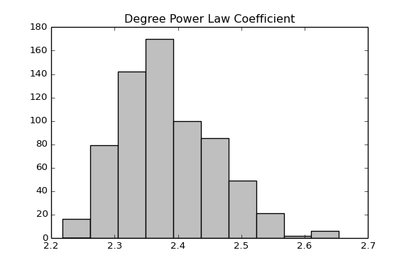
Figure 1: Illustration of the variance in power law coefficient ($\alpha$) for a population of over 700 Autonomous Systems (AS) graphs sampled at different time points. Few anomalous samples were removed from the original population.

	PA [3]	ERGM [25]	CL [1]	BTER [20]	KPGM [12]	mKPGM [16]	xKPGM
1. Learnable	$\times$	$\surd$	See note	See note	$\surd$	$\surd$	$\surd$
2. Scalable Learning	–	$\surd$	–	–	$\surd$	$\times$	$\surd$
3. Scalable Generation	$\times$	$\times$	$\surd$	$\surd$	$\surd$	$\surd$	$\surd$
4. Match Local Properties	$\times$	$\times$	$\times$	$\surd$	$\surd$	$\surd$	$\surd$
5. Capture Variance	$\times$	$\times$	$\times$	$\times$	$\times$	$\surd$	$\surd$

TABLE I: Comparison of existing graph generation models with the proposed xKPGM model. PA - Preferential Attachment, ERGM - Exponential Random Graph Models, CL - Chung-Lu, BTER- Block Two Erdös-Rényi, KPGM- Kronecker Product Graph Model, mKPGM- Mixed KPGM, xKPGM- Proposed Model. Note: The CL and BTER models can be used to generate a synthetic graph from a given real graph with approximately the same number of nodes, however it does not allow generation of arbitrary sized synthetic graphs.

In summary, the research community needs a scalable graph generative model which matches properties of real graphs, including the variance exhibited by a population of graphs. However, as shown in Table I, most existing graph generators lack in at least one of the desired characteristics listed above.

In particular, the Kronecker Product Graph Model (KPGM) [12] has been shown to satisfy some of the above properties. The multiplicative nature of the model allows for fast sampling of massive sized graphs and has been shown, both analytically and empirically, to generate graphs that follow many power-law characteristics for several global graph properties. Moreover, a method of moments based approach was proposed for parameter learning with KPGM [7], which allows it to scale to massive graphs. However, recent papers have identified few shortcomings of KPGM.

The single biggest argument made against KPGM is that they lack the ability to capture the natural variability observed in real world graphs [14, 21]. Researchers have shown that the synthetic graphs sampled from KPGM show little variation in terms of several graph properties. The problem is attributed to the fractal nature of growth in the generative model. The tied-KPGM (tKPGM) and the mixed-KPGM (mKPGM) are two variants proposed to alleviate the issues with KPGM [14]. However, as we demonstrate experimentally, these next generation models are also not expressive enough to model the natural variance in the data. Moreover, the estimation process using the simulated method of moments approach is expensive and not scalable to learning from massive graphs.

To alleviate the lack of variation in existing models, we propose a mixture based approach for graph generation using Kronecker product. In particular, this paper makes the following specific contributions:

1. We propose a mixture-model based Kronecker product graph model (xKPGM). We also show that the existing models are particular instantiations of the proposed xKPGM model.

2. We analytically examine the expected properties of the graph generated by the proposed model.

3. We derive expressions for the expectactions for several salient graph properties for our model. Using these expressions, we provide a method of moments based parameter learning algorithm for the proposed model.

4. We propose a random subgraph based method to evaluate generative models for graphs.

5. We show, analytically and empirically, that xKPGM matches the real graph properties and captures the natural variability in graphs more effectively than existing Kronecker models and other graph generative models.

II Related Work

Generative models for graphs has been a widely studied field for many decades. One of the earliest ones is the Erdős-Rényi model [18] which has obvious shortcomings as it fails to capture properties of real-world graphs. More recent models have focused on the preferential attachment property of nodes, i.e., new nodes tend to form edges with nodes with greater degree [3]. However, in such models, the graph is grown one node at a time, which makes them inherently serial and unscalable. Lately, there has been an emphasis on models which can be learnt from observed graphs. These include the Exponential Random Graph Models (ERGM) (also referred to as p* models) [25]. ERGM essentially defines a log linear model over all possible graphs $G$, $p(G|\theta)\propto exp(\theta^{T}s(G)$, where $G$ is a graph, and $s$ is a set of functions, that can be viewed as summary statistics for the structural features of the network. Another popular and well-known network models are Stochastic Block Models (SBM) [24] in which each node belongs to a cluster and the relationships between nodes are determined by their cluster membership. While conventional SBM are defined for non-overlapping community assignments, many overlapping or mixed variants have also been introduced [2]. Another relevant model is the Chung-Lu (CL) model [1] in which the probability of an edge is proportional to the product of the degrees of its end vertices. While CL model effectively captures the degree distribution, it performs poorly for other properties such as clustering coefficient. A recent extension to CL model, called the Block Two-Level Erdős-Rényi (BTER) model [20] is shown to match both the degree distribution and clustering coefficient on several graphs. However the BTER model is not truly generative as it only allows for creation of a synthetic graph which is exactly the same size as the observed graph. For generating arbitrary sized graphs one needs to provide parameters instead of learning them.

Kronecker product based generative models are increasingly becoming popular [12]. However, given their limited expressiveness [14, 21], several variants have been proposed [14, 15]. The most promising extension, mKPGM, is able to capture the variance in a graph population, however, the parameter estimation phase is expensive. We will be discussing the original model and two variants in more detail in the paper. There also have been other related papers that improve KPGM in other ways, e.g., the Multiplicative Attribute Graph Models [11].

III Background

In this section we introduce the various Kronecker product based models that have been proposed for modeling large graphs. For clarity, we will use the notation used in this section for the subsequent sections of the paper.

III-A Kronecker Product Graph Model

KPGM [12] is a fractal growth model. A graph $\mathcal{G}$ with $N$ nodes is obtained by first generating a $N\times N$ stochastic matrix (containing entries between 0 and 1). The edge between node $i$ and $j$ is independently (from other edges) generated using a Bernoulli trial with the $ij^{th}$ entry from the matrix. The generative algorithm starts with an initial matrix $\mathcal{P}_{1}=\Theta$, which is $b\times b$; typically $b$ is set to 2 or 3, e.g.:

$$\mathcal{P}_{1}=\Theta=\left[\begin{array}[]{cc}\theta_{11}&\theta_{12}\\ \theta_{21}&\theta_{22}\end{array}\right]$$ (1)

The algorithm takes repeated Kronecker product of $\mathcal{P}_{1}$ with itself to generate a larger matrix. For example,

$$\mathcal{P}_{n}=\underbrace{\mathcal{P}_{1}\otimes\mathcal{P}_{1}\otimes\ldots\otimes\mathcal{P}_{1}}_{n\text{ times}}$$ (2)

Note that the matrix $\mathcal{P}_{n}$ will have $b^{n}$ rows (and columns). This matrix is then used to generate a graph $\mathcal{G}=({\bf V},{\bf E})$ with nodes ${\bf V}=\{1,2,\ldots,N\}$. For each pair $(u,v)$, where $1\leq u,v\leq b^{n}$, a Bernoulli sample is generated with parameter $\mathcal{P}_{n}[u,v]$. If the sample is 1 (success), edge $(u,v)$ is added to ${\bf E}$. We denote this process as a realization of $\mathcal{P}_{n}$ to get the adjacency matrix, $A$ ($=R(\mathcal{P}_{n})$).

The KPGM model can assign a probability to a given graph $\mathcal{G}$ as long as the correspondence of nodes in $\mathcal{G}$ to the rows of $\mathcal{P}_{n}$ are given (denoted by $\sigma$). Given the KPGM model ($\mathcal{P}_{1}=\Theta$) and the correspondence function $\sigma$, the probability of an observed graph $\mathcal{G}=({\bf V},{\bf E})$ is given by:

$$P(\mathcal{G}|\Theta,\sigma)=\prod_{(u,v)\in{\bf E}}\mathcal{P}_{n}[\sigma(u),\sigma(v)]\prod_{(u,v)\notin{\bf E}}(1-\mathcal{P}_{n}[\sigma(u),\sigma(v)])$$ (3)

where $\mathcal{P}_{n}$ is derived from $\Theta$ using (2).

Given an observed graph $\mathcal{G}$, two approaches for learning the model parameters ($\Theta$) have been proposed. The first is an MLE approach that approximates computes the gradient of the log-likelihood of the graph (See (3)) [12]. Since the correspondence function $\sigma$ is unknown, the learning algorithm searches over the factorial possible permutations using Metropolis-Hastings sampling and then uses a gradient descent approach to update the parameters in $\Theta$. The second learning approach is based on method of moments [7]. This method avoids the issue of searching over the factorial space of permutations.

It has been shown that KPGM generates graphs which match real networks in terms of several properties such as skewed degree distribution, short network path length, etc. Moreover, the model allows very fast sampling of large graphs ($O(|{\bf E}|)$). However, recent work has identified several limitations with KPGM. Seshadri et al. [21] have shown that graphs generated from KPGM have 50-75% isolated vertices. Moreno et al. [14] have observed, both analytically and empirically, that graphs generated from KPGM do not capture the variability observed in the real networks expected to be generated from the same source. They have attributed this shortcoming to: (i) use of independent edge probabilities, (ii) fractal expansion, and (iii) small number of model parameters. In fact, after several Kronecker products, most entries in the eventual stochastic matrix tend to become homogeneous. This results in a lack of variance since all sampled graphs appear similar.

Moreno et al. [14] investigated several simple approaches to induce variability in KPGM generated graphs. These include using larger initiator matrices and sampling $\Theta$ from a distribution instead of using a point estimate. None of these variations induced significant variability in the sampled graphs. The same authors make the following key observation: For a graph $\mathcal{G}=({\bf V},{\bf E})$ generated by KPGM, $Var(|{\bf E}|)\leq\mathbb{E}[|{\bf E}|]$, independent of $n$. The authors empirically observed that in real networks, the estimated variance of the number of edges across multiple variations of the same graph (across time) is significantly greater than the mean. Thus KPGM cannot generate graphs with large variance.

III-B Tied Kronecker Product Graph Model

Moreno et al. [14] proposed a generalization of KPGM that allows larger variance in the properties of the graphs sampled from the model by inducing edge dependence in the generation process. In the generative process, an adjacency matrix is realized after each iteration from the current matrix $\mathcal{P}_{t}$, denoted as $R(\mathcal{P}_{t})$. The next stochastic matrix, $\mathcal{P}_{t+1}$ is obtained by performing a Kronecker product of the realized adjacency matrix and the initiator matrix, i.e., $\mathcal{P}_{t+1}=R(\mathcal{P}_{t})\otimes\mathcal{P}_{1}$. Note that for KPGM, only one realization is done (after the $n^{th}$ iteration). Thus, the final adjacency matrix can be obtained using recursive realizations and Kronecker products, i.e.,

$$A=\underbrace{R(\ldots R(R(\mathcal{P}_{1})\otimes\mathcal{P}_{1})\ldots)}_{n\text{ realizations}}$$ (4)

The above model is called tied KPGM or tKPGM since the realization at every step can also be thought of as tying the Bernoulli parameters. The authors show analytically that the variance for the expected number of edges in graphs generated using tKPGM is higher than KPGM, in fact the variance was higher than desired which motivated the variant discussed next.

III-C Mixed Kronecker Product Graph Model

The mixed KPGM or mKPGM variation allows the graph to grow as KPGM (without realizations) for first $l$ steps and then acts as tKPGM for remaining $n-l$ steps. mKPGM has an additional parameter $l$ which denotes the extent of tying in the model. Note that for $l=1$, mKPGM is equivalent to tKPGM and for $l=n$, mKPGM is equivalent to KPGM.

IV Natural Variability in Real Graphs

A vital requirement for any graph generative model is the ability of the model to capture the variability across multiple observed samples. In fact, both tKPGM and mKPGM were motivated due to the limited ability of previous models to capture this variability. Most generative graph models have focused on capturing the properties observed for a single instance. But such models are not equipped to model a set of graphs, assumed to be sampled from the same statistical distribution. In many real world applications, one can obtain multiple samples of graphs which would exhibit variance in the different properties. For example, a set of social networks of students for different colleges, or a set of citation networks collected for different decades or disciplines. We show one example in Figure 1 where we consider daily AS networks across several years. In general, obtaining such populations to study the variance is challenging.

In this paper, we address this challenge by generating random subgraphs of a given graph. For a given large graph, the idea is to extract subgraphs using a sampling strategy such that the properties of the original graph are preserved in the subgraph. Several such methods have been proposed in the literature [13, 9, 22]. In this paper we use a variant of the forest fire model to generate subgraphs. In this method, a random node is chosen and the neighborhood of the chosen node is traversed in a breadth first approach. Each outgoing edge from the node is added to the sample with a certain probability. The nodes at the end of the chosen edges are then further “burnt” and the “fire” is further spread.

To illustrate the variability we consider several publicly available real world graphs listed in Table II.

Name	Description	Nodes	Edges
as [23]	CAIDA AS Relationship Graph	6,474	13,233
ca-astroPh [23]	Collaboration network of Arxiv Astro Physics	18,772	396,160
elegans [6]	C. elegans metabolic network	453	4,596
hep-ph [23]	Citation network from Arxiv HEP-PH	34,546	421,578
netscience [17]	Coauthorship network of scientists	1,589	5,484
protein [10]	Protein interaction network for Yeast	1,870	4,480

TABLE II: Publicly available graph data sets used in the evaluation. More details available at http://www.cse.buffalo.edu/~chandola/research/bigdata2015graphs/info.html.

For each graph in Table II, we sample 200 subgraphs (number of nodes were typically 4 times less than the original number of nodes) using the forest-fire approach and measure characteristics of each subgraph. The empirical distribution for several characteristics are shown in Figure 2. We study the following five important characteristics: (i) power law coefficient ($\alpha$) of the degree distribution (ii) number of edges, (iii) number of triangles, (iv) average path length, and (v) average clustering coefficient.

Figure 2: Empirical distribution of graph characteristics for the graphs listed in Table II. The histogram is obtained by taking multiple random sub-graph samples and measuring five properties of the sub-graph.

The empirical distributions show that for most of the characteristics, the population of subgraphs exhibit significant variation. Moreover, the variation itself is not completely arbitrary, but in most cases, resembles standard distributions such as Gaussian or exponential.

V Proposed xKPGM Model

Existing Kronecker product based models are inadequate in capturing the natural variance that exists in graph populations. To address this issue, we propose a mixture-model based approach which allows capturing this variance. We call the proposed model xKPGM, where the ‘x’ signifies that all variants of KPGM discussed in Section III are specific instantiations of xKPGM.

The key idea behind xKPGM is to use $k$ ($k\geq 1$) initiator matrices of possibly different sizes. The graph generation follows similar iterative expansion as seen in other models discussed in Section III with the difference that at any iteration one of the $k$ initiator matrices is randomly chosen for the Kronecker product by drawing a sample from a Multinomial distribution parameterized by a $k$ length probability vector ${\bm{\pi}}$ ($\sum_{i}^{k}\pi_{i}=1$). Similar to mKPGM, there is a parameter $l$ ($1\leq l\leq k$) such that for first $l$ iterations no realization (or tying) is performed while from iteration $l+1$, parameter tying through realizations is employed.

To illustrate the impact of using multiple initiator matrices instead of a single matrix, we generate multiple synthetic graphs using different generative models. We use the following two initiator matrices:

$$\Theta_{1} =\left(\begin{array}[]{cc}0.95&0.60\\ 0.60&0.20\end{array}\right) \Theta_{2} =\left(\begin{array}[]{cc}0.99&0.20\\ 0.20&0.70\end{array}\right)$$ (9)

Figure 3: Variation of number of edges for synthetic graphs with $2^{10}$ nodes generated by mKPGM and xKPGM for varying levels of tying ($l$). Note that $l=1$ indicates purely tied model (tKPGM) and $l=10$ indicates purely untied model (KPGM). The error bars are computed by generating 2000 samples for each value of $l$.

These exact matrices have been used in previous papers [14] for conducting empirical simulations for mKPGM and other variants. The mean and the variance for the number of edges across the simulations is shown in Figure 3 which illustrates that the variability (in terms of the number of edges) for samples generated by mKPGM is low for higher values of $l$ ($\geq 6$). In fact, the variance becomes negligible for KPGM ($l=10$). For very low values of $l$ the variability is very high. On the other hand, xKPGM generates samples with much more stable variability across $l$. We observe that for xKPGM, the variance is generally higher when $\pi=0.5$, though it also depends on the individual initiator matrices. We observe similar behavior for other properties (clustering coefficient, etc.) as well.

V-A xKPGM Sampling Algorithm

The steps for sampling a graph in xKPGM are shown in Algorithm 1. Note that the algorithm needs following inputs: $k$ initialization matrices, ${\Theta_{1},\Theta_{2},\ldots,\Theta_{k}}$, a $k$ length vector ${\bm{\pi}}$, the number of iterations $n$, and the level of tying $l$. The number of rows (and columns) for each matrix $\Theta_{i}$ is denoted as $b_{i}$.

V-B Interchangeability in Kronecker Products

We make use of the following important result [8] for Kronecker matrices. For two matrices $A$ and $B$:

$$A\otimes B=M(B\otimes A)N$$ (10)

where $M$ and $N$ are permutation matrices which merely change the order of rows and columns, respectively. In other words, the above result means that the Kronecker product is commutative as long as we allow changing of labels of nodes, which is irrelevant in our case. Since in Algorithm 1, the order of rows and columns is not important, one can use this result in the purely untied setting. In Algorithm 1, the graph generated using any arbitrary sequence of initialization matrices is equivalent to the following canonical sequence:

$$\underbrace{(\Theta_{1}\otimes\Theta_{1}\ldots)}_{n_{1}\text{ times}}\otimes\underbrace{(\Theta_{2}\otimes\Theta_{2}\ldots)}_{n_{2}\text{ times}}\otimes\ldots\otimes\underbrace{(\Theta_{k}\otimes\Theta_{k}\ldots)}_{n_{k}\text{ times}}$$

The above observation allows us to arrive at several important results later, because it simplifies the analysis, especially, in the untied setting for xKPGM, where arbitrary sequences of initialization matrices can be represented using the above canonical sequence. In fact, the next result follows from this observation.

V-C Generating Graphs of Arbitrary Sizes

The input $n$ determines the eventual size of the graph in terms of the number of nodes ($|{\bf V}|$). For a simple case where all initialization matrices are of the same size ($b_{i}=b,\forall i$), the size of the graph will be $b^{n}$. In general, expected number of nodes will be $\prod_{i=1}^{k}b_{i}^{n\pi_{i}}$.

Note that existing Kronecker based models are limited to generating graphs with number of nodes as exact powers of $b$ (typically set to 2 or 3). On the other hand, xKPGM can generate graphs with number of nodes, which in principle, need not be restricted to the exact powers of $b$. Thus, by using initialization matrices of varying sizes, xKPGM can generate graphs with more number of possibilities for the number of nodes. For example, if we use two initialization matrices of sizes 2 and 3 and if $N$ can be factorized as $2^{a}3^{b}$, then one can set $\pi_{1}=\frac{a}{a+b}$ and $\pi_{2}=\frac{b}{a+b}$ and generate a graph using Algorithm 1 with $N$ expected number of nodes.

Input: $\Theta_{1},\Theta_{2},\ldots,\Theta_{k},{\bm{\pi}},n,l$

Output: Adjacency matrix $A$

1 $\mathcal{P}\leftarrow 1$

// Untied Phase

2 foreach $t=1$ to $l$ do

3       $i\sim Multinomial({\bm{\pi}})$

4       $\mathcal{P}\leftarrow\mathcal{P}\otimes\Theta_{i}$

5      

// Tied Phase

6 foreach $t=l+1$ to $n$ do

       $A\leftarrow R(\mathcal{P})$;

        // $R$ - Realization

7       $i\sim Multinomial({\bm{\pi}})$

8       $\mathcal{P}\leftarrow A\otimes\Theta_{i}$

9      

10$A\leftarrow R(\mathcal{P})$

return $A$

Algorithm 1 Graph Generation Algorithm for xKPGM

V-D Relationship to Existing Models

If $k=1$ and $l=1$, xKPGM is equivalent to tKPGM. Similarly, for $k=1$ and $l=n$, xKPGM is equivalent to KPGM. For $k=1$ and for all other values of $l$ ($1\leq l<n$) xKPGM is equivalent to mKPGM. Thus all existing Kronecker product based graph models are specific instantiations of xKPGM.

Model	$\mathbb{E}[{\bf E}]$	$var[{\bf E}]$
KPGM	$S_{\Theta}^{n}$	$S_{\Theta}^{n}-S_{\Theta^{2}}^{n}$
tKPGM	$S_{\Theta}^{n}$	$S_{\Theta}^{n-1}(S_{\Theta}^{n}-1)\frac{S_{\Theta}-S_{\Theta^{2}}}{S_{\Theta}-1}$
mKPGM	$S_{\Theta}^{n}$	$S_{\Theta}^{n-1}(S_{\Theta}^{n-l}-1)\frac{S_{\Theta}-S_{\Theta^{2}}}{S_{\Theta}-1}+(S_{\Theta}^{l}-S_{\Theta^{2}}^{l})S_{\Theta}^{2(n-l)}$
xKPGM (purely tied)	$(\pi_{1}S_{\Theta_{1}}+\pi_{2}S_{\Theta_{2}})^{n}$	$(\pi_{1}(S_{\Theta_{1}}-S_{\Theta_{1}^{2}})+\pi_{2}(S_{\Theta_{2}}-S_{\Theta_{2}^{2}})+\pi_{1}\pi_{2}(S_{\Theta_{1}}-S_{\Theta_{2}})^{2})\sum_{j=1}^{2(n-1)}(\pi_{1}S_{\Theta_{1}}+\pi_{2}S_{\Theta_{2}})^{j}$
xKPGM (untied)	$S_{\Theta_{1}}^{\pi_{1}n}S_{\Theta_{2}}^{\pi_{2}n}$	$S_{\Theta_{1}}^{\pi_{1}n}S_{\Theta_{2}}^{\pi_{2}n}-S_{\Theta_{1}^{2}}^{\pi_{1}n}S_{\Theta_{2}^{2}}^{\pi_{2}n}$

TABLE III: Comparison of $\mathbb{E}[{\bf e}]$ and $var[{\bf e}]$ for Kronecker models. $S_{\Theta}$, $S_{\Theta_{1}}$ and $S_{\Theta_{2}}$ denote the sum of values of $\Theta$, $\Theta_{1}$ and $\Theta_{2}$. $S_{\Theta^{2}}$, $S_{\Theta^{2}_{1}}$ and $S_{\Theta^{2}_{2}}$ denote the sum of squares of values of $\Theta$, $\Theta_{1}$ and $\Theta_{2}$.

Kronecker product models have been analyzed in terms of the expected number of edges for the generated samples. In Section VI, we provide similar expressions for other graph properties as well. In Table III, we list the expressions for the expectation and variance for the number of edges for xKPGM and compare them with other models. The derivation is omitted in the interest of space though the key is to use the Observation V-B along with the fact that the expectation of an edge between a pair of nodes is equal to the corresponding value in the final stochastic matrix.

VI Properties of xKPGM Graphs

In this section we provide expressions for expectations of four key properties for graphs, viz., i) edges, ii) hairpins (or 2-stars), iii) tripins (or 3-stars), and iv) triangles. These four properties provide an understanding of local structure of the samples. Moreover, we will be using the expressions to estimate the model parameters in Section VII. For simplicity we assume that all $k$ initiator matrices are of size $2\times 2$ and are of the following form: $\Theta_{k}=\left(\begin{array}[]{cc}a_{k}&b_{k}\\ b_{k}&c_{k}\end{array}\right)$. The derivation for expected values in the purely untied ($l=n$) setting closely follows the line of argument taken for pure KPGM [7] (Section 3) and makes use of Observation V-B. The expressions are provided in Table IV.

$2\mathbb{E}[{\bf E}]$	$=$	$\prod_{i=1}^{n}(a_{i}+2b_{i}+c_{i})^{\pi_{i}n}-\prod_{i=1}^{n}(a_{i}+c_{i})^{\pi_{i}n}$
$2\mathbb{E}[{\bf H}]$	$=$	$\prod_{i=1}^{n}((a_{i}+b_{i})^{2}+(b_{i}+c_{i})^{2})^{\pi_{i}n}-2\prod_{i=1}^{n}(a_{i}(a_{i}+b_{i})+c_{i}(c_{i}+b_{i}))^{\pi_{i}n}-\prod_{i=1}^{n}(a_{i}^{2}+2b_{i}^{2}+c_{i}^{2})^{\pi_{i}n}+2\prod_{i=1}^{n}(a_{i}^{2}+c_{i}^{2})^{\pi_{i}n}$
$6\mathbb{E}[{\bf T}]$	$=$	$\prod_{i=1}^{n}((a_{i}+b_{i})^{3}+(b_{i}+c_{i})^{3})^{\pi_{i}n}-3\prod_{i=1}^{n}(a_{i}(a_{i}+b_{i})^{2}+c_{i}(b_{i}+c_{i})^{2})^{\pi_{i}n}$
	$-$	$3\prod_{i=1}^{n}(a_{i}^{3}+c_{i}^{3}+b_{i}(a_{i}^{2}+c_{i}^{2})+b_{i}^{2}(a_{i}+c_{i})+2b_{i}^{3})^{\pi_{i}n}+2\prod_{i=1}^{n}(a_{i}^{3}+2b_{i}^{3}+c_{i}^{3})^{\pi_{i}n}$
	$+$	$5\prod_{i=1}^{n}(a_{i}^{3}+c_{i}^{3}+b_{i}^{2}(a_{i}+c_{i}))^{\pi_{i}n}+4\prod_{i=1}^{n}(a_{i}^{3}+c_{i}^{3}+b_{i}(a_{i}^{2}+c_{i}^{2}))^{\pi_{i}n}-6\prod_{i=1}^{n}(a_{i}^{3}+c_{i}^{3})^{\pi_{i}n}$
$6\mathbb{E}[{\bm{\Delta}}]$	$=$	$\prod_{i=1}^{n}(a_{i}^{3}+3b_{i}^{2}(a_{i}+c_{i})+c_{i}^{3})^{\pi_{i}n}-3\prod_{i=1}^{n}(a_{i}(a_{i}^{2}+b_{i}^{2})+c_{i}(b_{i}^{2}+c_{i}^{2}))^{\pi_{i}n}+2\prod_{i=1}^{n}(a_{i}^{3}+b_{i}^{3})^{\pi_{i}n}$

TABLE IV: Expressions for ${\bf E}$ - num. edges, ${\bf H}$ - num. hairpins, ${\bf T}$ - num. tripins and ${\bm{\Delta}}$ - num. of triangles

Note that the expression for $\mathbb{E}[{\bf E}]$ here is slightly different from a similar expression in Table III. The reason is that in Table IV we do not count the self-loops and count each edge only once.

VII Parameter Estimation

The parameters of xKPGM are the elements in the $k$ initiator matrices and the vector ${\bm{\pi}}=\pi_{1},\pi_{2},\ldots,\pi_{k}$. We describe a method of moments based approach to estimate these parameters from a given observed graph. The graph is characterized using a set of statistics (or moments). In this paper we have used the same moments as used in the past for KPGM estimation (edges, hairpins, tripins, and triangles) [7]. The idea is to find the model parameters such that the expected moments for the model match closely with the moments computed from the observed graph within an optimization procedure. Each moment is denoted as $F_{i}$ and the computed moment for an observed graph $\mathcal{G}$ is denoted as $F_{i}^{*}$. The estimation method searches for the parameters $\Theta_{1},\Theta_{2},\ldots,{\bm{\pi}}$ which minimize the following objective function:

$$f({\Theta},{\bf F}^{*})=\sum_{i=1}^{|{\bf F}|}w_{i}\left(\frac{F_{i}^{*}-\mathbb{E}[F_{i}|\Theta]}{F_{i}^{*}}\right)^{2}$$ (11)

where $w_{i}$ indicates a weight assigned to the $i^{th}$ moment. In this paper we have used equal weights, however, they can be used to assign more emphasis on certain moments. Note that the above objective function can be easily extended to learn from multiple graphs by replacing the observed moment $F_{i}$ in (11) with the average moment value across all $p$ observed graphs, i.e., $\widetilde{F}_{i}=\frac{1}{p}\sum_{\mathcal{G}}F_{i\mathcal{G}}$.

For xKPGM in a purely untied setting ($l=n$), we have expressions for each of the moments as functions of the parameters (See Table IV). We plugin these expressions into a gradient based optimizer (e.g., fmincon function available in Matlab) to get the optimal parameter values.

Note that the above estimation algorithm can be extended to more general settings of purely untied xKPGM such as using initiator matrices of larger sizes ($>2$ and using initiator matrices with different sizes, by deriving the appropriate expressions similar to the ones listed in Table IV. For the tied setting ($l<n$), obtaining such closed form expressions is challenging. However, one could use the simulated method of moments approach which was originally proposed for mKPGM [16].

VIII Computational Complexity

Generating a graph of size $N$ using the learnt initiator matrices using Algorithm 1 requires $n=\log_{2}{N}$ Kronecker products and $l$ intermediate realization followed by $N^{2}$ bernoulli trials for the final realization. In the original KPGM paper [12], the authors propose a sampling strategy which is linear in the number of edges, however, that method requires one to specify the number of edges desired in the graph. For xKPGM the generation is dominated by the final $O(N^{2})$ realization step. However, given that the realizations are independent, efficient distributed implementations can be devised.

The parameter estimation using the method of moments allows scalable training. The only compute intensive phase is the computation of the moments for the observed graph, which is done once. The objective function can be computed in $O(1)$ time, independent of the size of the observe graph. In contrast, the simulated method of moments, used by mKPGM, requires computation of the moments for the generated graph multiple times at each iteration of the gradient descent, making it unscalable to large graphs. The number of iterations required by the fmincon minimizer will depend on the number of model parameters, which increases linearly with the number of initiator matrices ($k$).

IX Experimental Results

We present results on several publicly available network data sets (See Table II). The evaluation has two objectives. We first show that the parameters learnt for xKPGM using the algorithm sketched in Section VII allow a more accurate modeling of the observed graph, compared to other Kronecker based models.

IX-A Parameter Estimation

For each graph in Table II, we estimate parameters using Matlab fmincon with 5000 initial values with constraints that elements of the initiator matrices are between 0 and 1 and $a_{i}>c_{i}$. We train xKPGM with two initiator matrices of size $2\times 2$ and other models (KPGM, tKPGM, mKPGM) using one initator matrix of size $2\times 2$, using the objective function in (11) and the four moments listed in Table IV. For mKPGM and tKPGM, we use implementation provided by the authors [16]. For KPGM, we used the direct optimization method [7].

IX-B Matching Moments

The objective function values (see (11)) for the different methods are shown in Figure 4. For every data set, xKPGM gives the best estimation in terms of the objective function, especially for ca-astroPh, netscience, protein, and hep-ph data sets. The relative performance of other models varies across the different data sets. In general, we observe that the objective function value improves as the tying level ($l$) decreases and is best when $l=1$, i.e., tKPGM.

Figure 4: Comparing xKPGM with other models in terms of the objective function value obtained after training.

IX-C Impact of Number of Initiator Matrices

To understand how the choice of $k$, i.e., the number of initiator matrices, impacts the performance of the model, we compared the objective function obtained by training the xKPGM model using different values of $k$. The results for three graphs are shown in Figure 5. In all three cases, increasing $k$ from 1 to 2 results in a significant improvement in the objective function. For two of the graphs (netscience and protein), increasing $k$ beyond 2 does not show any further improvements. However, for the $as$ graph, higher values of $k$ show improvement in the objective function.

Figure 5: Performance of xKPGM using different number of initiator matrices ($k$). Note that $k=1$ is KPGM.

IX-D Variability of Generated Samples

The second set of experiments attempt to understand the variability in the samples generated by the xKPGM and other Kronecker models. For each model, we use the estimated parameters and generate 200 samples with the same sample size that was used to generate the subgraphs in Section IV. For each sample we measure five salient properties similar to Figure 2 and plot the distribution across the samples. The distributions for cit-hepPh is shown in Figure 6.

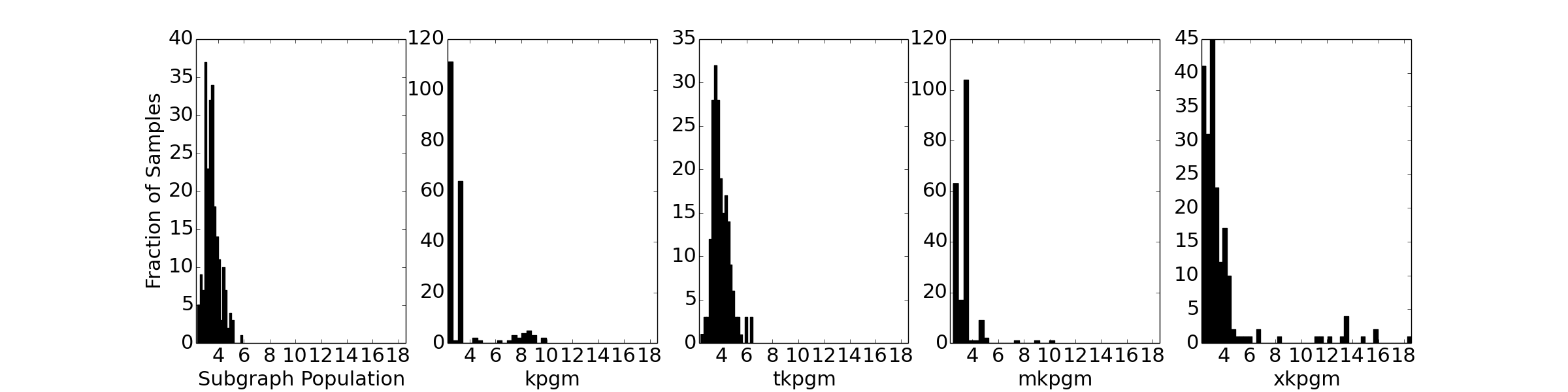
(a) Power Law Coefficient of Degree Distribution

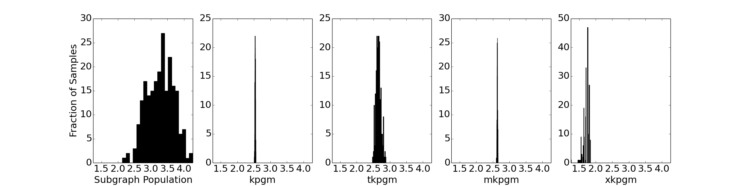
(b) Average Path Length

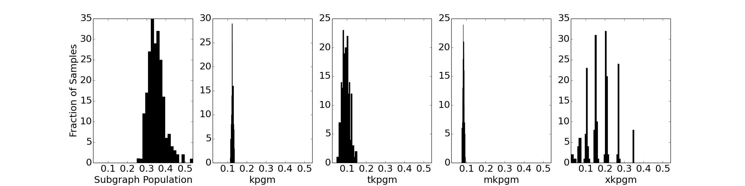
(c) Average Clustering Coefficient

Figure 6: Distribution of network characteristics for samples using the models trained on cit-hepPh data. The first plot in each row is the distribution for the subgraph population discussed in Section IV.

In the results shown in Figure 6, both KPGM and mKPGM exhibit almost negligible variability for almost all of the network properties. In fact, it is evident that the variability increases as we decrease $l$ from $n$ (KPGM) to $1$ (tKPGM). xKPGM shows most variability, and in many cases approximately matches the variability of the subgraph population (degree distribution, average clustering coefficient).

IX-E Comparison with BTER

As noted earlier, the BTER model allows generating a synthetic graph which approximates an observed graph. However, by design, BTER can generate graphs of approximately the same size (nodes and edges) as the observed graph. Using the available implementation, we observed that while BTER matches the degree distribution and the clustering coefficient, the generated graphs show minimal variation for a set of samples generated using the same observed graph. For example, for the ca-astroPH graph, 200 simulations using BTER resulted in graphs with number of edges in the range: $196156\pm 208$ and the average clustering coefficient in the range: $0.3265\pm 0.0013$.

X Conclusions

We propose a new generative model, xKPGM, for graphs based on mixture of Kronecker models. The model induces variability by incorporating multiple initiator matrices strung together using a random multinomial trial, while retaining the strong features of KPGM, such as scaling to massive graphs. We provide analytical expressions for various characteristics of the generated graphs which allows us to estimate the parameters using a method of moments approach. The mixture approach allows us to devise a scalable method of moments based learning method (similar to KPGM) while achieving better variance (similar to mKPGM).

We show, both analytically and through experiments, that xKPGM is able to learn a model which best matches the moments of the observed graph (See Figure 4) and also induces variability (See Figure 6) which aligns with the natural variability observed in real graphs (See Figure 2). To better evaluate the variability of generative graph models we have come up with a sub-graph based method. Using this method we show that the proposed model provides a robust variance across multiple graph properties. We also provide comparisons with the state of art generative models and show that xKPGM outperforms them both in terms of matching the graph properties and the variance in the population.

References

- [1] W. Aiello, et. al., “A random graph model for power law graphs,” Experiment. Math., 10(1), 53–66, 2001.
- [2] E. M. Airoldi, et. al. Mixed membership stochastic blockmodels. J. Mach. Learn. Res., 9:1981–2014, 2008.
- [3] A.-L. Barabasi and R. Albert. Emergence of scaling in random networks. Science, 286(5439):509–512, 1999.
- [4] J. Casas-Roma, et al., “An algorithm for k-degree anonymity on large networks,” in ASONAM, 2013.
- [5] V. Chandola, et. al., “Knowledge discovery from massive healthcare claims data,” in KDD, 2013.
- [6] J. Duch and A. Arenas. Community detection in complex networks using extremal optimization. Physical Review E, 72:027104, 2005.
- [7] D. F. Gleich and A. B. Owen. Moment-based estimation of stochastic kronecker graph parameters. Internet Mathematics, 8(3):232–256, 2012.
- [8] H. V. Henderson and S. R. Searle. The vec-permutation matrix, the vec operator and kronecker products: a review. Linear and Multilinear Algebra, 9(4):271–288, 1981.
- [9] C. Hübler, et. al. Metropolis algorithms for representative subgraph sampling. In ICDM, 2008.
- [10] H. Jeong, et. al. Lethality and centrality in protein networks. Nature, 411:41–42, 2001.
- [11] M. Kim and J. Leskovec. Multiplicative attribute graph model of real-world networks. Internet Mathematics, 8(1-2):113–160, 2012.
- [12] J. Leskovec, et. al. Kronecker graphs:An approach to modeling networks. J. Mach. Lear. Res., 11:985–1042, 2010.
- [13] J. Leskovec and C. Faloutsos. Sampling from large graphs. In Proceedings of the SIGKDD pages 631–636, 2006.
- [14] S. Moreno, et. al. Tied kronecker product graph models to capture variance in network populations. In IEEE Communication, Control, and Computing (Allerton), 2010.
- [15] S. Moreno, et. al. Block kronecker product graph model. In Workshop on Mining and Learning from Graphs, 2013.
- [16] S. I. Moreno, et. al. Learning mixed kronecker product graph models with simulated method of moments. In SIGKDD, pages 1052–1060, 2013.
- [17] M. E. J. Newman. Finding community structure in networks using the eigenvectors of matrices. Phys. Rev. E, 74:36–104, 2006.
- [18] P. Erdős and A. Rényi. On the evolution of random graphs. In Publication of the Mathematical Institute of the Hungarian Academy of Sciences, pages 17–61, 1960.
- [19] A. Sanzgiri, A. Hughes, and S. Upadhyaya, “Analysis of malware propagation in Twitter,” in IEEE SRDS, 2013.
- [20] C. Seshadhri, et. al., “Community structure and scale-free collections of erdös-rényi graphs,” CoRR, 2011.
- [21] C. Seshadhri, et. al. An in-depth analysis of stochastic Kronecker graphs. Journal of the ACM, 60(2), 2013.
- [22] H. Sethu and X. Chu. A new algorithm for extracting a small representative subgraph from a very large graph. CoRR, 2012.
- [23] SNAP: Stanford network analysis platform. http://snap.stanford.edu/data/index.html.
- [24] T. A. Snijders and K. Nowicki. Estimation and prediction for stochastic blockmodels for graphs with latent block structure. Journal of Classification, 14(1):75–100, 1997.
- [25] S. Wasserman and P. Pattison. Logit models and logistic regressions for social networks. Psychometrika, 61(3):401–425, 1996.