Emergence of Landauer Transport from Quantum Dynamics: A Model Hamiltonian Approach

I Introduction

The interest in time dependent (TD) quantum transport has been growing with the ever improving technologies. Although nanoscale devices have long been fabricated and characterized, it is only recently that the challenge of combining the spatial with temporal resolution to capture short time phenomena was achieved. Ultrafast experiments were initially restricted to solid state thin films but are now increasingly manifested in molecular scale materials. Irrespective of the system, the electrons are first to react to the ultrashort perturbations and may or may not attain a dynamic equilibrium depending on the time span of the disturbance. Theoretical methods for exploring the steady-state electron flow (dynamic equilibrium) in mesoscopic systems is a mature field and the challenge is gradually shifting towards molecular and atomic scale systems. Although several of the established mesoscale methods are transferable to the sub-nanometer scale, junction conductance is completely oblivious to it. Quantum tunneling, which dominates the transport characteristics in sub-nanoscale junctions, requires a different set of theoretical tools.

The scenario becomes more complicated if the flow of electrons acquire a time dependence, for example, if they are driven by an alternating voltage or if they interact with an ultrashort laser pulse. In general, it is difficult to employ a steady-state formalism to describe transienceCarey et al. (2017) but the reverse mapping can be natural and convenient. With this motivation, the theory of TD quantum transport has become an active area of research during the past few decades. Early efforts were directed towards developing a TD Green function framework that would converge seamlessly into a Landauer type conductance formula under certain conditionsJauho, Wingreen, and Meir (1994). The advent of powerful computers lead to numerical recipes for computing TD Green’s functionsHou et al. (2006); Moldoveanu, Gudmundsson, and Manolescu (2007); Prociuk and Dunietz (2008); Gaury et al. (2014); Ridley, Mackinnon, and Kantorovich (2015); Ding, Xiong, and Dong (2016); Popescu and Croy (2016) in open systems. Computationally expensive time dependent density functional theory (TDDFT) was also used as an approach to calculate the TD current for both openWang, Hou, and Zheng (2013) and closed systemsStefanucci and Almbladh (2004). In the simplest implementation, the one-particle density matrix was propagated in time by a driving term in a tight-binding model with mean-field interactions at the level of adiabatic local density approximationSánchez et al. (2006). First-principles realization of a similar methodology was reported recentlyMorzan et al. (2017). A quasi-steady-state current-voltage characteristics was obtained in a finite sized nano junction using TDDFT on a tight-binding model within a microcanonical approach which agreed with static scattering calculationsDi Ventra and Todorov (2004); Bushong, Sai, and Di Ventra (2005). More recently, with a more generalized implementation of the above framework, Ercan and Anderson showed that the emergence of TD current and local occupation functions are structure dependentErcan and Anderson (2010). TDDFT based studies were reported, for example, to explore the transient current in molecular devices under ac biasBaer et al. (2004); Wu et al. (2005); Ke et al. (2010), to calculate currents due to a pulsedZhu et al. (2005) or an exponentially turned on voltageWang et al. (2011), or an optical pulseGalperin and Tretiak (2008), and to illustrate dynamic suppression of current due to charge build upEvans and Voorhis (2009). The effects of the lead sizeCheng, Evans, and Van Voorhis (2006) and the TDDFT exchange and correlation functionals on the transient current Evans, Vydrov, and Van Voorhis (2009) were explored in refs. Cheng, Evans, and Van Voorhis, 2006; Evans, Vydrov, and Van Voorhis, 2009. Open boundary conditions were implemented within TDDFT using a modified Crank-Nicholson algorithm and a stationary current was achieved for one dimensional model systemsKurth et al. (2005). Using a microcanonical framework within TDDFT, similarities between pressure gradients in classical fluid flow and transient electronic current in nanoscale junctions were illustratedSai et al. (2007). Comparison of transport characteristics as obtained from static DFT + NEGF and TDDFT using complex absorbing potentials to tackle open boundary conditions were performed in benzene-dithiolate and bipyridine junctions with gold electrodesVarga (2011). A combination of TDDFT and NEGF within the wide-band limit approximation was also used to investigate transient transport characteristics in realistic molecular junctionsZheng et al. (2007, 2010); Zhang, Chen, and Chen (2013). Recently, a TDDFT approach based on grids in real space and real time was applied to a system of conjugated molecules and reliability of the concept was establishedSchaffhauser and Kümmel (2016). A combination of quantum dissipative theory and TDDFT was also utilized to study optically induced transient current in a weakly coupled molecular deviceCao et al. (2015). In another recent study, the dependence of early transient transport on the symmetry of the initial state of the system was exploredTu et al. (2016). Simulations using density functional based tight binding (DFTB), which are an order of magnitude cheaper than TDDFT, also appeared to capture the transient current dynamics although only at low biasesWang and May (2011).

Mapping the real-space to state-space representation and propagating the density matrix via the Louiville-von Neumann equation of motion can also capture the transient transport and, moreover, allow modeling of complex multi-terminal finite but realistic junctionsZelovich, Kronik, and Hod (2014); Chen, Hansen, and Franco (2014); Zelovich, Kronik, and Hod (2016); Zelovich et al. (2017). Other formalisms include a many body path integral Monte Carlo approach that, when applied on a quantum system coupled to a phonon bath exhibited a TD current that reached a non-equilibrium stationary state after the initial transienceMühlbacher and Rabani (2008). In another many body approach the Kadanoff-Baym equations for the NEGF were propagated in time resulting in the inclusion of electronic correlations and the ability to include TD external perturbationsMyöhänen et al. (2009). This method not only estimated the transient current and molecule charging timesMyöhänen et al. (2009) but was also able to address the molecule-lead effect on the screening and the relaxation timesMyöhänen et al. (2012). The effect of electronic correlations (both electron-electron and electron-vibration) on the transient current was also explored through multilayer multiconfiguration time dependent Hartree theoryWang and Thoss (2013).

Most of the transient current features reported in the literature can however be captured within a wave function approach (rather than density propagation), which (subject to certain approximations discussed below) is computationally cheaper. In addition, the interaction terms of the molecular bridge with the electrodes can be extracted from first-principles calculations (formally at any level of accuracy) and incorporated into the dynamics. In this article, we formulate and investigate quantum transport by applying the time dependent Schrödinger equation to a model Hamiltonian. Our Hamiltonian is an extended version of the one used earlier to study heterogeneous electron transferRamakrishna, Willig, and May (2001). We focus on simple two-terminal model devices, where the electrodes and the bridge are replaced by uniformly spaced quasi-continuum (QC) and a set of discrete energy levels respectively. Our model Hamiltonian consists of separate sets of energy levels corresponding to each sub-system (left and right lead, molecular bridge) and coupling terms between the molecule and the quasi-continua. At the initial time, the populations in the quasi-continua are determined by the Fermi-Dirac distribution (FDD) with a common Fermi level ($E_{f}$).

We construct the most general expression for the TD current ($I_{L}$) in terms of the rate of change of population in the left QC (LQC), which has two components $I_{in}$ and $I_{out}$ corresponding to the incoming and the outgoing populations, respectively. Our calculations demonstrate (1) at early times $I_{in}$ and $I_{out}$ oscillate with a damped frequency and amplitude, (2) after a certain time, both $I_{in}$ and $I_{out}$ settles into a constant value and $I_{L}$ matches exactly with steady-state Landauer current. We term the commencement of the overlap between the two currents (exact and Landauer) as the onset of the Landauer regime and are the first ones to show the natural emergence of Landauer transport from a first-principles quantum dynamical picture sans prior assumptions. The initial frequency and amplitude of the oscillations and the timescale of the onset of the Landauer regime depend strongly on the electronic coupling strength of the molecule bridge with the electrodes. We are able to define and extract a time dependent transmission (and reflectance) function and illustrate that it transitions into a steady state after the onset of the Landauer regime. Finally, we focus on the importance of our framework by comparing the current calculated by our exact expression to the Landauer current when time dependence in the electronic coupling between the bridge and the electrodes is turned on. Additionally, we examine the charge dynamics when hot-electrons are generated via plasmonic excitations in one of the electrodes.

The paper is organized as follows: In section II we introduce the quantum dynamical model and the main working equations. Subsequently, we provide the results and discuss them extensively in section III. Finally, in section IV, we conclude the paper with a brief summary and outlook of our work.

II Formalism

II.1 Transport from quantum dynamics

A two-terminal device is modeled by three sub-systems - two leads, each replicated by a uniform QC and a bridge state (BS) described by a discrete set of energy levels. Thus, the Hamiltonian of the above system is written as:

$$\begin{split}H=\displaystyle\sum_{k_{l}}\epsilon_{k_{l}}\mid k_{l}~{}\rangle\langle~{}k_{l}\mid+\displaystyle\sum_{k_{r}}\epsilon_{k_{r}}\mid k_{r}~{}\rangle\langle~{}k_{r}\mid+~{}\displaystyle\sum_{m}\epsilon_{m}\mid m~{}\rangle\langle~{}m\mid\\ +\bigg{(}\displaystyle\sum_{k_{l}}V_{k_{l}m}\mid k_{l}~{}\rangle\langle~{}m\mid+\displaystyle\sum_{k_{r}}V_{k_{r}m}\mid k_{r}~{}\rangle\langle~{}m\mid+~{}h.c\bigg{)}\end{split}$$ (1)

where $\epsilon_{k_{l/r}}$ and $\mid k_{l/r}\rangle$ are the energy eigenvalues and eigenstates respectively of the electrodes. $\epsilon_{m}$ and $\mid m\rangle$ are the stationary energy level and state of the BS. $V_{k_{l/r}m}$ are the terms between coupling the BS to the quasi-continua. The total wave function is written as:

$$\begin{split}\mid\psi(t)_{total}\rangle=\displaystyle\sum_{m}c_{m}(t)e^{-i\omega_{m}t}\mid m\rangle+\displaystyle\sum_{k_{l}}c_{k_{l}}e^{-i\omega_{k_{l}}t}\mid k_{l}\rangle+\displaystyle\sum_{k_{r}}c_{k_{r}}e^{-i\omega_{k_{r}}t}\mid k_{r}\rangle,\end{split}$$ (2)

where $c_{k_{l/r}}$ and $c_{m}$ are the complex amplitudes corresponding to each eigenstate in the QCs and the BS respectively and $\omega_{x}=\epsilon_{x}/\hbar,x\in m,k_{l},k_{r}$. Substituting equation 2 in the time dependent Schrödinger equation and using the orthogonality of the $\mid x\rangle$ we obtain:

$$\begin{split}i\hbar~{}\dot{c_{k_{l}}}=\displaystyle\sum_{m}c_{m}V_{k_{l}m}e^{i(\omega_{k_{l}}-~{}\omega_{m})t}\end{split}$$ (3)

$$\begin{split}i\hbar~{}\dot{c_{k_{r}}}=\displaystyle\sum_{m}c_{m}V_{k_{r}m}e^{i(\omega_{k_{r}}-~{}\omega_{m})t}\end{split}$$ (4)

$$\begin{split}i\hbar~{}\dot{c_{m}}=\displaystyle\sum_{k_{l}}V_{k_{l}m}c_{k_{l}}e^{i(\omega_{k_{m}}-\omega_{k_{l}})t}+\displaystyle\sum_{k_{r}}V_{k_{r}m}c_{k_{r}}e^{i(\omega_{k_{m}}-~{}\omega_{k_{r}})t}.\end{split}$$ (5)

Again, from the Heisenberg equation of motion we derive the following equation for the expectation value of the rate of change of occupancy in the LQC:

$$\begin{split}\langle\dot{n}_{L}^{k^{0}_{l/r}}\rangle~{}=~{}-\dfrac{i}{\hbar}\big{[}n_{L}^{k^{0}_{l/r}},H\big{]}~{}=~{}\dfrac{2}{\hbar}Im\big{\{}\displaystyle\sum_{k_{l}}V_{k_{l}m}c_{k_{l}}^{*}c_{m}e^{i(\omega_{k_{m}}-~{}\omega_{k_{l}})t}\big{\}},\end{split}$$ (6)

where $\langle n_{L}^{k^{0}_{l}}(t)\rangle=\displaystyle\sum_{k_{l}}|c_{k_{l}}(t)|^{2}$ with the initial condition - ONE eigenstate is populated @t=0 and the expectation value is obtained from that TD wave function. Formally, equation 6 can be rewritten in a condensed form as:

$$\begin{split}\langle\dot{n}_{L}^{k^{0}_{l/r}}\rangle~{}=~{}\dfrac{2}{\hbar}Im\big{\{}\displaystyle\sum_{k_{l/r}}T_{k_{l/r}m}\big{\}}f_{k^{0}_{l/r}}~{}=~{}S_{k^{0}_{l/r}}f_{k^{0}_{l/r}},\end{split}$$ (7)

where $f_{k^{0}_{l/r}}$ is the Fermi-Dirac occupancy (@t = 0) of a particular eigenstate in either QC. We justify the factorization of equation 7 as a product of Fermi-Dirac occupancy and a reflectance/transmission function in the appendix. If the initially occupied state is in the LQC (RQC), $S_{k^{0}_{l}}$ ($S_{k^{0}_{r}}$) is a reflectance (transmission) function. As the initial state of the full system is an incoherent superposition of the electrode states, the observables are determined by time propagating the wave function for a range of initial electrode states and summing the initial-state-dependent-observables with weights determined from a FDD. The electronic current in the LQC, denoted as $I_{L}$, can now be split into two contributions, one corresponding to initial population in the LQC ($I_{out}$) and the other for the population originating in the RQC ($I_{in}$):

$$\begin{split}I_{out}~{}=~{}\sum_{k_{l}^{0}}\langle\dfrac{d}{dt}n_{L}^{k^{0}_{l}}\rangle~{}=~{}\sum_{k_{l}^{0}}S_{k^{0}_{l}}f_{k^{0}_{l}},\\ I_{in}~{}=~{}\sum_{k_{r}^{0}}\langle\dfrac{d}{dt}n_{L}^{k^{0}_{r}}\rangle~{}=~{}\sum_{k_{r}^{0}}S_{k^{0}_{r}}f_{k^{0}_{r}},\end{split}$$ (8)

where $\sum_{k_{l}^{0}}$ and $\sum_{k_{r}^{0}}$ represents the summation over all initial conditions associated with the initial populations at LQC and RQC respectively. The total current in the left electrode $I_{L}$ can then be written as:

$$\begin{split}I_{L}=I_{out}-I_{in}=\sum_{k_{l}^{0}}S_{k^{0}_{l}}f_{k^{0}_{l}}-\sum_{k_{r}^{0}}S_{k^{0}_{r}}f_{k^{0}_{r}}.\end{split}$$ (9)

which is our most general expression for the TD current valid at all times.

III Results and Discussion

III.1 Dynamics

We investigate the population dynamics within our single-particle framework by introducing a finite number of particles into our microcanonical (total energy and the number of particles is fixed) system. At zero bias, the equilibrium Fermi levels ($E_{f}$) in both quasi-continua are identical and are placed at the center of the range of QC levels (0 - 1.2 eV with a spacing of $\Delta_{QC}=0.005$ eV unless or otherwise mentioned) to avoid band edge effects and allow comparison with the analytical data. We restrict our time propagation to $t<t_{r}(=\frac{2\pi\hbar}{\Delta_{QC}})$, where $t_{r}$ is the recurrence time - defined as the time limit until which a QC acts as a realistic continuumRamakrishna, Willig, and May (2001). The maximum level spacing we use in our calculations is $\Delta_{QC}=0.005$ and so we cutoff all our quantum dynamics simulation at 800 femtoseconds (fs) or even before. The population ($\langle{n}_{x}^{k^{o}_{l/r}}\rangle;x\in$ BS, LQC, RQC) as a function of time in the various sub-systems for energy independent coupling strengths ($V_{k_{l/r}m}$) and BS on-resonance with $E_{f}$, is illustrated in Figure Supplementary Information (SI)-2. A certain amount of population is transferred from the QCs to the empty BS until the populations in the sub-systems achieve a dynamic equilibrium. The overall population decay rate of the two QCs are identical since there is no external bias on the system and $V_{k_{l}m}=V_{k_{r}m}$. The saturation population at the BS and the equilibration time are determined by $V_{k_{l/r}m}$, the density of states ($\rho$) in the quasi-continua ($\rho={\Delta_{QC}}^{-1}$) and the alignment of the BS with $E_{f}$. In the example shown here the saturation population is 0.5 and the equilibration time is $\sim 391$ fs. The saturation population on the BS is directly proportional to $V_{k_{l/r}m}$ and is maximum if the BS is on-resonance with $E_{f}$.

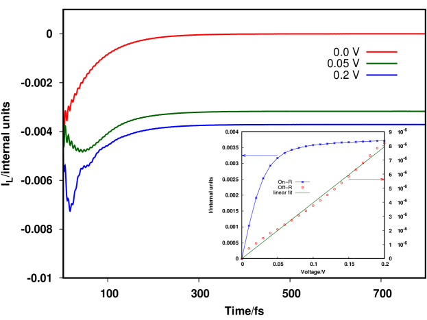
Figure 1: $I_{L}$ as a function of time for different external voltages as mentioned in the legends. Inset: current-voltage characteristics when BS is on (on-R) and off-resonance (off-R) with $E_{f}$. QC levels run from $0-1.2$ eV with a spacing of 0.005 eV with equilibrium Fermi level at 0.6 eV. BS is positioned at 0.6 eV and 1.0 eV for the on-R and off-R cases respectively. $V_{k_{l/r}m}$ = 0.002 eV for both the arrangements.

We introduce an external bias ($V_{B}$) by modifying the local chemical potential (CP) in the QCs by $\pm V_{B}/2$, where the positive sign corresponds to a higher CP at the left ($\mu_{1}=E_{f}+V_{B}/2$) compared to that in the right electrode ($\mu_{2}=E_{f}-V_{B}/2$). In the presence of bias voltage, $I_{L}$ (defined in equation 9) saturates, after short time fluctuations, to a non-zero as seen in Figure 1. As expected $I_{L}$ settles to 0 (red) at $V_{B}$ = 0 V. $I_{L}$ is negative at long times because $V_{B}$ is positive resulting in steady-state unidirectional population flow from the LQC to the right QC (RQC). Similar quasi-steady currents in closed systems have been reported earlier in several TD quantum transport calculations on model junctionsZhu et al. (2005); Kurth et al. (2005); Bushong, Sai, and Di Ventra (2005); Sánchez et al. (2006); Zheng et al. (2007); Varga (2011); Yam et al. (2011); Wang et al. (2011); Schaffhauser and Kümmel (2016). The long time limit of $I_{L}$ is the non-equilibrium steady-state current and it is evidently bias dependent as shown in the inset of Fig. 1. Near resonance (blue line in the inset of Figure 1) we observe a sigmoidal current-voltage characteristics. The same voltage dependence was found in early steady-state calculations of the transportDi Ventra M, Pantelides, and Lang (2000); Pal and Pati (2011) and of current-driven dynamicsAlavi et al. (2000). The trend is readily explainable through the analytical theory of Alavi et al. (2000) to mirror the eigenvalue structure of the bridging molecule, with the steepness of the sigmoidal curve determined by the resonance lifetime. If the BS is outside the window ($E_{f}+0.4$ eV) of $\mu_{1}$ and $\mu_{2}$ (off-R) the current-voltage alliance is linear (red dots with a green fit), which is consistent with off-resonance tunneling trendsPal and Pati (2010). Thus our formulation, along with our definition of current approves the steady-state current-voltage relationship reported in the literature. It is however interesting to note that the increase in the steady-state current with $V_{B}$ is maximum in the on-R model, where BS $=(\mu_{1}+\mu_{2})/2$. Shifting the BS (denoted by $\Delta$) diminishes the slope of the sigmoidal current-voltage curve as shown in Figure SI-3 although the long-time limit current at higher applied biases converges to the same value for all BS locations.

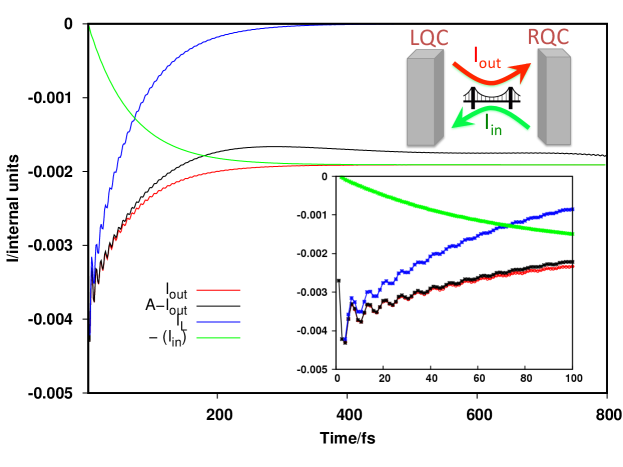
Figure 2: Current dynamics at the LQC and its $I_{out}$ and -$I_{in}$ components. Bridge level (BS) is on-resonance with the equilibrium $E_{f}$ of the QCs. The definition of the components are provided in the text. Inset: Transient current at very early times. The parameters are identical to the on-R model in Figure 1.

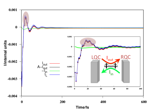
Figure 3: Dynamical current at the LQC and its $I_{out}$ and -$I_{in}$ contributions. Inset: Current at very early times. Parameters are identical to Figure 2 but BS is located at 0.7 eV.

III.2 Non-equilibrium Steady State

I_L consists of 2 components, one ($I_{out}$) corresponding to initial population in the left and the other ($I_{in}$) to the initial population in the right QC. In Figure 2, we show the $I_{L}$ and its components at $0~{}V$ for the on-R model introduced in section III.1. $I_{out}$ is always negative because the population flux originating in the LQC leaks out of it at all times. In contrast, $I_{in}$ is always positive since it adds population to the LQC. However, we plot $-(I_{in})$ to illustrate that $I_{in}$ and $I_{out}$ settle into an equal and opposite value and at the same time, which is 391 fs for this particular arrangement of energy levels. Beyond this point, the transient features in the current (and its components) disappears and the rate of population exchange attains a steady value (for $V_{B}\neq 0$V,) replicating the time-independent non-equilibrium steady-state current. Thus, commencing from a quantum dynamical description of population transport between the LQC-BS-RQC we arrive at a time independent charge flow, which is a measurable quantity.

It is however interesting to note that $I_{out}$ oscillates at early times (inset of Figure 2) due to significant backscattering from the BS to the LQC, whereas $I_{in}$ exhibits a relatively smooth trend. This behavior is consistent with an earlier observation that an electron when traveling from a narrow conductor to a wide lead suffers from minimal reflectionSzafer and Stone (1989) but the vice-versa is not trueDatta (1997); Di Ventra (2008). The segment of population originating in the RQC and leaking out of LQC is negligible because coupling between the sub-systems is relatively weak. Oscillations in $I_{in}$ however observed if the coupling strength is significantly increased (for e. g., a 5 fold increase) as illustrated in the results of Figure SI-4.

III.3 Comparison with an Analytical Theory

We derive an analytical expression for $I_{out}$ to arrive at a structure for a more generalized expression for the time-dependent electron transport, which is later shown to reduce to the Landauer expression in the steady state. We are interested to explore the physics of the analytical expression, though they are admittedly approximate, as the truncated recursions ignore the population dynamics of the initially unoccupied states in the dynamical expression for the initially occupied states. This neglect propagates even through the dynamics of the initially unoccupied states that are derived subsequently from the incomplete expression for the initially occupied states as elaborated in the appendix.

The black line (denoted as A-$I_{out}$) in Figure 2 corresponds to $I_{out}$ calculated from the analytical expression (derived in the appendix) for the on-R arrangement. Our analytical theory agrees well with the numerical calculations (red) for the initial few tens of fs (inset of Figure 2) after which the high-frequency current fluctuations evaluated from either expression are damped and additionally, they start to deviate from each other. This discrepancy arises because we stop at the first recursion to get to a closed form of the analytical expression as detailed in the appendix. A consequence of this approach is the exclusion of at least two higher order processes: (1) influence of the initially unoccupied LQC levels on the rate of population leakage at the initially occupied level in the same electrode, (2) the population dynamics of a specific initially unoccupied LQC level being exclusively related to the population of the initially occupied level and not on the rest of the unoccupied LQC levels. Both the above-mentioned higher order processes, which are unaccounted for in our simplified analytical expression, involve backscattering of the BS population into the LQC levels. The time scale of backscattering associated with a single LQC level can be approximated by $2\pi\hbar/\Delta_{BS-\epsilon_{k_{l}}}$, where $\Delta_{BS-\epsilon_{k_{l}}}$ is defined as the energy difference between BS and $\epsilon_{k_{l}}$. However, it is difficult to nail the time scale of the overall backscattering that disturbs the initial overlap between the numerical and the analytical currents because of the summation over all $\epsilon_{k_{l}}$ in $I_{out}$(equation 8).

In the off-resonance case (Fig. 3), where BS $=E_{f}+0.1$ eV, the analytical expression for I_out (black) is in excellent agreement with its numerical counterpart (red). This result could be anticipated - the backscattering of BS population into LQC in this situation is inefficient because of lack of BS population in the first place (note - BS is on-resonance with initially unoccupied LQC levels). As a result, the higher order processes ignored by our restricting the analytical solution to the first recursion, are unable to play a dominant role in the overall population dynamics. We also note (see Figure 3) that $I_{L}$ is strongly dominated by I_out in the off-resonance case. Due to lack of occupied RQC levels around BS, I_in is negligibly small at early time and converges to zero as time progresses. It is also interesting to note that $I_{L}$ in this setup reverses its direction (as marked by shaded oval areas in Figure 3) before the onset of steady state. To analyze this behavior we replot the dynamical current alongside the rate of change of population in the LQC level resonant with BS (marked by a magenta line ‘X’ in the schematic of Figure SI-5). Part of the BS population is backscattered into ‘X’, culminating in LQC population gain until $\sim$150 fs before the rate of gain starts to drop off. We establish this by tracking $I_{out}$ in Figure SI-5 , which changes its sign synchronously with $I_{L}$ around 20 fs. In the inset of the same figure, we further observe the on-resonant LQC level gains population on a similar time scale, thus supporting the sign reversal of $I_{out}$. When the bridge level is below the Fermi level (BS $=E_{f}-0.4$ eV) the current dynamics (Figure SI-6) is similar to Figure 2. The initial oscillations in $I_{L}$ are, however, less frequent and more damped, possibly due to a sizable amount of population exchange between the initially filled levels of both the quasi-continua and the BS. The analytical expression in this scenario agrees with the numerical $I_{out}$ at early time scales and displays low frequency oscillation instead of transitioning into a steady state. Overall, we do establish that our truncated analytical expression is able to capture the transience although does not perform well in the long-time limit. However, the structure of our analytical formula cements the foundation for the rest of the interrogations in the article.

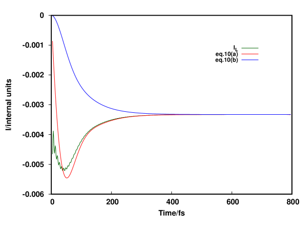
Figure 4: $I_{in}^{Land}$ and $I_{out}^{Land}$ as calculated from an approximate Landauer type equation 10. The exact $I_{L}$ is also plotted to illustrate the emergence of the Landauer regime. The model and parameters of Figure 1 are used but with $V_{B}$ = + 0.06 V

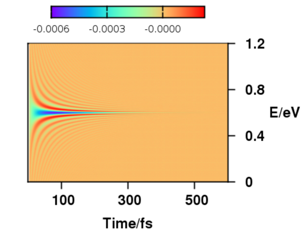
Figure 5: Difference of the time dependent functions $S_{k^{0}_{l}}$($\epsilon$,t) and $S_{k^{0}_{r}}$($\epsilon$,t). The model and parameters of Figure 1 are used here.

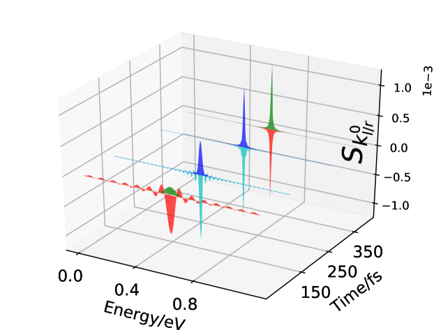
Figure 6: Time dependent reflectance(red and cyan) and transmission(blue and green) functions, $S_{k^{0}_{l/r}}$($\epsilon$,t). The model and parameters of Figure 1 are used here.

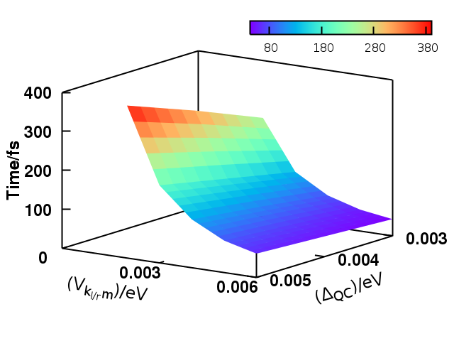
Figure 7: Onset of Landauer regime for a range of symmetric coupling strength between the bridge and the QC and energy levels spacing in the QCs. The bridge level is on-resonance with the E_F.

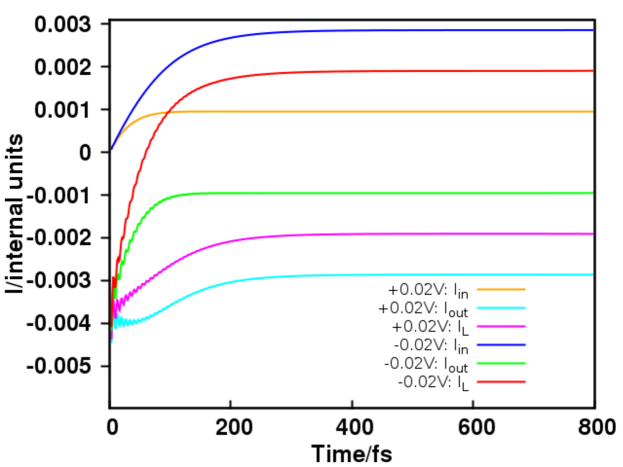
Figure 8: Onset of Landauer regime for a range of symmetric coupling (C) strength between the bridge and the QC and energy levels spacing (S) in the QCs. The bridge level is on-resonance with $E_{f}$.

III.4 Onset of the Landauer Regime

The analytical solution of $I_{out}$ in equation 26 (Appendix) indicates that the FDD can be factored out as a time independent segment of the function. $I_{in}$ is also expressible similarly (equation 31 in Appendix) and exploiting this structural form we approximate I_L as:

$$I_{L}=\displaystyle\sum_{k_{l}^{0}}S_{k^{0}_{l}}\big{(}f_{k^{0}_{l}}-f_{k^{0}_{r}}\big{)}=I^{Land}_{out}$$ (10a)

$$=\displaystyle\sum_{k_{r}^{0}}S_{k^{0}_{r}}\big{(}f_{k^{0}_{r}}-f_{k^{0}_{l}}\big{)}=I^{Land}_{in}$$ (10b)

The equations above are very similar to the Landauer formula:

$$\begin{split}I_{L}=\displaystyle\sum_{\epsilon=-\infty}^{+\infty}T(\epsilon)\bigg{[}f_{l}(\epsilon)-f_{r}(\epsilon)\bigg{]},\end{split}$$ (11)

where $f_{l/r}(\epsilon)$ is the FDD at the left/right electrode. Comparing equations 10 and 11, we have that $S_{k^{0}_{l/r}}$ takes the role of a reflectance/transmission function in our formalism. In Figure 4 we plot $I_{out}^{Land}$ and $I_{in}^{Land}$ for the on-R model, which are approximate Landauer currents given by equation 10. Red, blue and dark-green curves corresponds to $I_{out}^{Land}$, $I_{in}^{Land}$, and $I_{L}$ (equation 9) respectively. All the calculations are performed with $V_{B}=+0.06$ V as equations 10a and  10b go to zero at all times when $V_{B}=0$ V. We clearly observe that the approximate Landauer type expressions are devoid of any rapid oscillations and are unable to capture the transient current. Despite this drawback, the current via this expression converges to the correct $I_{L}$ rendering the Landauer type equations invalid prior to the onset of the steady state at 391 fs. Thus, we are able to capture the natural emergence of the Landauer transport from a quantum dynamical framework without the prior assumption of time independent charge flow between the sub-systems. This is the central result of our efforts here, which was possible only because of our analytical expressions that allowed us to define the Landauer $I_{L}$ and compare it with the numerically exact $I_{L}$.

To analyze the emergence of the Landauer regime, we plot the difference of the transmission ($S_{k^{0}_{r}}$) and the reflectance function ($S_{k^{0}_{l}}$) as a function of time in Figure 5. At an early time the difference as a function of energy is finite but this quantity goes to zero after the onset of the Landauer regime with $S_{k^{0}_{l}}=S_{k^{0}_{r}}$ at all energies, further illustrated in Figure 6. $S_{k^{0}_{r}}$ is plotted in green and blue in Figure 6 whereas red and cyan curves show $S_{k^{0}_{l}}$. $S_{k^{0}_{l}}$ values are negative because it corresponds to population decrease in the LQC. Both transmission and reflectance functions at early times are spread over multiple energy levels before settling down to equal and opposite Lorentzian functions (last data point) centered around the BS after the population exchange attains a dynamic equilibrium. The full-width at half maxima (fwhm) of the Lorentzian depends on the electronic coupling between the QC and the BS. After the onset, one of the $S$’s in equation 9 can be factored out resulting in the Landauer type formulas of equation 10. Increasing $V_{k_{l}m}$ results in a steady-state $S_{k^{0}_{r}}$ (and also $S_{k^{0}_{l}}$) with a larger fwhm as shown in Figure SI-7a and an early Landauer onset (Figure SI-7b) as detailed in the next section.

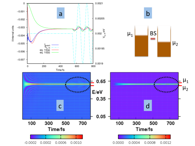
Figure 9: (a)Comparison of exact $I_{L}$ with approximate Landauer type equation 10 in the presence of time dependent coupling ($V_{k_{l/r}m}$ (cyan curve plotted against right ordinate) between the bridge and the electrodes. (b) The position of BS and the chemical potentials are shown using schematics for the two respective situations. Bias = $\mu_{1}-\mu_{2}$ = 0.05 V. (c) Reflectance as a function of time and energy. (d) Transmittance as a function of time and energy. Dotted ovals in (c) and (d) indicate the region where the coupling is time dependent. $\mu_{1}$ and $\mu_{2}$ are marked by short red dashes in (c) and (d).

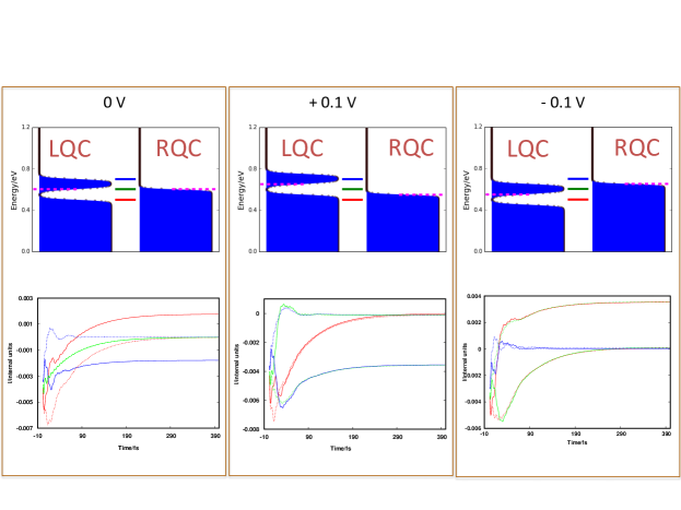
Figure 10: I_L in the absence (dotted lines) and presence (solid lines) of hot electrons that are generated via plasmon decoherence in the LQC. Blue, green and red lines in the top panel represent the position of BS and the same colors are correspondingly used to plot the dynamical current in the bottom panel.

III.5 Controlling the Onset Time

We now proceed to systematically calculate the onset time of the Landauer regime as a function of the coupling strength and the energy level spacing of the QCs for the on-resonant case and present it in the form of a 3D plot in Figure 7. We define the onset of Landauer regime, $t_{L}$, as the time when $I_{L}$ in equation 9 goes to zero when $V_{B}=0$ V. For a symmetric coupling of BS with the QCs, $t_{L}$ is inversely proportional to $V_{k_{l/r}m}$; for example, $t_{L}$ is $\sim$ 391 and 82 fs for coupling strengths of 0.002 and 0.005 eV respectively. In the weak coupling regime, $t_{L}$ decreases as the energy levels in the QC are more closely spaced but as $V_{k_{l/r}m}$ gets stronger $t_{L}$ becomes independent of the level spacing. Between the two, $t_{L}$ has a stronger dependence on $V_{k_{l/r}m}$ than $\Delta_{QC}$ because the rate of population exchange between the sub-systems is controlled predominantly by the coupling strength. Computing the dependence of $t_{L}$ on $V_{k_{l/r}m}$ and QC level spacing using the approximate Landauer expression of equation 10 with a small bias of $+0.02$ V (Figure SI-8) reveals that the trend is qualitatively similar to Figure 7.

Despite being a purely theoretical aspect - we find it interesting that the individual contributions $I_{in}$ and $I_{out}$ attain the non-equilibrium steady state at the same time, only at $V_{B}=0$ V (Figure 2). When biased, the QC which has larger initial population in the energy levels close to BS, takes more time to attain the steady state. For example, when $V_{B}=+0.02$ V, $I_{out}$ (cyan curve in Figure 8) takes a much longer time to settle into a steady state whereas $I_{in}$ (orange curve in Figure 8) flattens out much earlier. The trend is reversed at $V_{B}=-0.02$ V where $I_{out}$ (green) transitions into the dynamic equilibrium much earlier that $I_{in}$(blue). However, $t_{L}$, which marks the onset of $I_{L}$ steady-state is independent of $V_{B}$. By contrast to the results of Figure 4, the individual contributions $I^{Land}_{in}$ and $I^{Land}_{out}$ in equation 10 transition into the steady state at the same time ($=t_{L}$) even if $V_{B}\neq$ 0 V. In experiments, the measurements will detect $I_{L}$ only but $t_{L}$ may continuously vary in situations such as in a scanning tunneling microscope (STM)-break junction approach, where the interaction strength between the bridge and the electrode changes along the course of the experiment.

III.6 Time Dependent Coupling

We next investigate the effectiveness of the Landauer formula in the presence of a TD perturbationPeskin (2017) for example, when a vibrational wave packet is excited in the bridging molecule, its distance from either electrode varies sinusoidally as a function of timeKaun and Seideman (2005) and so also would the electronic coupling matrix elements. We introduce this time dependence into our model by adding a term to the coupling (perturbation to $V_{k_{l}m}$ and $V_{k_{r}m}$ are out of phase by $\pi$) after the system settles into the Landauer regime. The red and green curves in Figure 9(a), which are calculated using equations 10a ($I_{Land}^{out}$) and  10b ($I_{Land}^{in}$) respectively, overlap with $I_{L}$ (blue curve) after $t_{L}$ and before the perturbation is applied. In Figure 9(b) we provide a schematic used for the calculations, which is identical to the on-R model mentioned in section III.1. As soon as the time dependent term in $V_{k_{l/r}m}$ is switched on, $I_{in}^{Land}$ and $I_{out}^{Land}$ drifts away from $I_{L}$ both in terms of amplitude and phase. $I_{out}^{Land}$ underestimates the current with a lower peak value as compared to $I_{L}$ whereas $I_{in}^{Land}$ overestimates. $I_{out}^{Land}$ is ahead in phase compared to $I_{L}$ and $I_{in}^{Land}$ is behind it. The disagreement between the analytical and numerically exact currents indicate the incompleteness of the Landauer expression when the coupling is time dependent.

To account for the disparities between the two Landauer currents of Figure 9(a) we analyze the response of $S_{k^{0}_{r}}$ and $S_{k^{0}_{l}}$ to the sinusoidal component of the $V_{k_{l/r}m}$. After the time dependent term in the coupling is switched on, $S_{k^{0}_{r}}$ fluctuates about BS (located at 0.6 eV in Figure 9(d)), the region indicated by dotted oval lines. In contrast, $S_{k^{0}_{l}}$ values at $\epsilon_{k_{l}}$ far off from BS also gains a time dependence (Figure 9(c)). It is essential to note that equations 10 and 11 reduce to:

$$I_{L}=\displaystyle\sum_{\epsilon_{k_{l}}=\mu_{1}}^{\epsilon_{k_{l}}=\mu_{2}}T(\epsilon_{k_{l}})\bigg{[}f_{l}(\epsilon_{k_{l}})-f_{r}(\epsilon_{k_{r}})\bigg{]}.$$ (12)

at low temperatures, when the Fermi-Dirac distribution approaches a step function and thus, the terms inside the parenthesis go to zero for $\mu_{2}<\epsilon_{k_{l}}<\mu_{1}$. As a result equation 10a captures the portion of the TD fluctuations in $S_{k^{0}_{l}}$ only within the range $\mu_{1}-\mu_{2}$ and misses the rest. However, equation 10b is able to capture the entire time dependence of $S_{k^{0}_{r}}$, which exclusively lies within the range $\mu_{1}-\mu_{2}$. This explains the existence of a higher peak in $I_{in}^{Land}$ and a smaller one in $I_{out}^{Land}$, with $I_{L}$ peaking between the two $I^{Land}$ currents. Thus, our analysis elucidates the central reason behind the deficiency of the Landauer expression in this situation - the starkly different response of the reflectance and the transmission function to the time dependent coupling.

III.7 Hot-electron Dynamics

In a scanning tunneling microscope, hot-electrons are created through plasmon decoherence when a laser is incident on a plasmonic tip. When the STM is engaged to a sample with monolayer of molecules hot electrons tunnel if they find suitable pathways such as molecular orbitals, giving rise to an additional current Pal et al. (2015). In order to model this process using our time dependent framework, we assume the existence of hot electrons in the LQC. We borrow an analytical expression for the distribution from our previous workKornbluth, Nitzan, and Seideman (2013); Pal et al. (2015) to investigate the transient hot-electron dynamics. The electrons in the RQC follow a pure FDD. We calculate $I_{L}$ from equation 9 for different BS positions, green for on-resonance and red (blue) for 0.1 eV below (above) the equilibrium Fermi level. Using the same colors in Figure 10, we plot $I_{L}$ as a function of time in the presence (absence) of hot electrons with solid (dotted) lines. The solid blue lines in the bottom panel of Figure 10(a) indicate that when BS is 0.1 eV above $E_{f}$, current flows from LQC to RQC whereas when it is 0.1 eV below $E_{f}$, the electronic population flows from RQC to the empty levels in the LQC in the steady state (red solid). Thus, even at 0 V hot electrons generate a finite current, the direction of which depends on the position of BS. As expected, in the absence of hot electrons, $I_{L}$ (represented by dotted lines) goes to zero at steady-state in Figure 10(a) irrespective of BS location. In the same figure, when BS is on-resonance with the equilibrium Fermi level, $I_{L}$ in the presence and absence of hot electrons (solid and dotted green) overlap with each other. This occurs possibly due to the proximity of BS to the tail of either the FDD or the hot electron distribution.

At a finite bias ($+0.1$ V), the current may be suppressed to zero when plasmons (and subsequently hot electrons) are excited in the LQC, for example, red and green solid lines in Figure 10(b). This happens because in both cases LQC and RQC levels close to BS are populated to similar extent; almost filled in red and almost empty for green. Similar considerations explain the results shown as blue and green solid lines in Figure 10(c). In the same figure, the population flows from the right to the left QC (red solid) giving rise to positive $I_{L}$ when BS is below the Fermi level. This happens because LQC has vacant levels close to BS where the population from RQC can flow into. In the presence of bias (Figure 10(b) and (c)), as expected from earlier sections, significant current flows in the absence of hot electrons only when BS lies within the window of $\mu_{1}$ and $\mu_{2}$. For all the cases considered here, $I_{L}$ transitions into the non-equilibrium steady state regime within few hundreds of fs and we verified that it converges to the Landauer current thereafter. This reinforces the validity of estimating the hot electron current via the Landauer expression in a STM tip-sample junction when the tip is excited by a continuous wave (CW) laser passed through a 80 Hz optic chopperPal et al. (2015). The CW laser is thus focussed on the STM tip for a few milliseconds during which the dynamical hot electron current would surely transition into the Landauer regime.

IV Conclusions

To summarize, we have devised a first-principles quantum dynamical framework for time dependent charge transport in a representative electrode-molecule-electrode arrangement. A quasi-continuum of evenly spaced energy levels and a single level depict the electrodes and the molecule respectively. Our approach is based on propagation of the single particle time dependent Schrödinger wave function of a model Hamiltonian. Our calculations reveal a transient charge flow at early time scales prior to the onset of a steady state. Upon biasing, the steady-state current (defined as the rate of charge flow from the left electrode) attains a nonzero constant value and exhibits a qualitatively similar current-voltage characteristics as that obtained via the popular Landauer formula. To gain further insight into these results, we derive a formally exact analytical formula for the portion of the current due to population originating from the left electrode, which shows excellent agreement with the numerical data at early time scales. We construct a closed form approximation by truncating higher order processes in our exact analytical form, and illustrate the emergence of high order processes at long time, manifested as deviation of the closed form approximation from the numerical results. The structural form of the analytical expression reveals that the outgoing current can be written as the initial occupancy multiplied by a transmission or reflectance function. Exploiting this observation, we rewrite the time dependent current in terms of an approximate Landauer style expression and illustrate that it matches the exact current (obtained from the most generalized definition) after the population dynamics settles into a steady state. We term this the onset of the Landauer regime, where, analogous to the Landauer formula, the net current in the left electrode can be expressed as a sum over the transmission (or reflectance) function weighted by the respective difference in the Fermi function occupancies. In-depth analysis points out that the transmission and reflectance functions transition into a time independent equal and opposite quantities after the onset. The onset time is however dependent on the coupling strength between the BS and the QCs and the QC level spacing with stronger coupling leading to faster onset of the Landauer regime. This behavior is explained in terms of rapid population exchange between the various subsystems.

When the coupling between the BS and the QCs is time-dependent, for example, when a vibrational wave packet is triggered in the bridge of a molecular scale junction the numerically exact dynamical current deviates from the Landauer currents. Discrepancies are recorded both in amplitude and phase of the current and the disagreement is associated with the distinctly dissimilar response of the transmission and the reflectance function to the time dependence of the coupling. In the transmission case, the time dependent fluctuations occur only at energy levels close to BS whereas in the reflectance case the time varying coupling seems to have an effect at energy levels away from the BS. Through our formalism we are able to visualize hot-electron dynamics, which is again a time dependent phenomenon. We predict flow of electrical current in an unbiased junction triggered solely by hot-electrons that are created from plasmon decoherences in metal nanoconstructs (such as a STM tip). Similarly, the current in a biased junction can be suppressed by exciting hot-electrons in one of the electrodes. In both scenarios, we show the importance of the presence of an appropriate bridging level that mediates the population exchange between the electrodes. We further show that the hot-electron dynamics settles into a steady state within few hundreds of femtoseconds, after which the Landauer expression gives realistic values for the current. Thus, we find that the current generated via tunneling hot-electrons (created from laser excitations) can be estimated by the conventional Landauer formula. One of our goals in future research in this area would be to calculate the current under similar conditions but for realistic molecular junctions by extracting the parameters of the model Hamiltonian from first-principles simulations. Our work will thus have important implications for fundamental investigations in molecular optoelectronics.

Appendix: Analytical expressions for the microscopic currents

We start from the differential equations for the TD amplitudes of $C_{k_{l}}(t)$, $C_{k_{r}}(t)$ and $C_{m}(t)$ namely equations (3 - 5) in the text. Substitution, integration and by application of the initial condition $C_{k_{l}}(t=0)=\sqrt{f_{k_{l}}}$, yields [see equation 3]

$$\dot{C}_{k_{l}}(t) = -\frac{{|v|}^{2}}{\hbar^{2}}\left(\int_{0}^{t}dt^{\prime}\,exp[-(A+iB)(t-t^{\prime})]\,C_{k_{l}}(t^{\prime})\right.$$ (13)

$$+\left.\sum_{k_{l}^{\prime}\neq k_{l}}e^{i\omega_{k_{l}}t}\int_{0}^{t}dt^{\prime}\,exp[-(A+i\omega_{m})(t-t^{\prime})-i\omega_{k_{l}^{\prime}}t^{\prime}]C_{k_{l}^{\prime}}(t^{\prime})\right).$$

where $A=\frac{\pi v^{2}\rho}{\hbar}$, $B=(\omega_{m}-\omega_{k_{l}})$ and $\rho$ is the density of states in the right electrode. The density of states is inversely related to the quasicontinuum spacing i.e., $\rho={\Delta_{QC}}^{-1}$, where $\Delta_{QC}$ is the energy spacing between quasicontinuum levels. In arriving at the above we have made use of the Poisson summation Lighthill (1970), $\sum_{k_{r}}e^{-i\omega_{k_{r}}(t-t^{\prime})}=2\pi\hbar\delta(t-t^{\prime})$, which is valid for an infinitely wide, uniform quasicontinuum of electrode levels, or the wide band limit (WBL). As the integro-differential equation obtained cannot be solved analytically, we attempt a recursive solution by ignoring levels that are initially unoccupied thus obtaining a closed form solution for the single level in the left electrode that is initially occupied. In other words, we assume that $C_{k_{l}^{\prime}}(t)\approx 0$ in Equation (13) obtaining

$$\dot{C}_{k_{l}}(t)\approx-\frac{{|v|}^{2}}{\hbar^{2}}\int_{0}^{t}dt^{\prime}\,exp[-(A+iB)(t-t^{\prime})]\,C_{k_{l}}(t^{\prime}).$$ (14)

Equation (14) is expected to be valid only in the short time limit. At long times neglecting the initially unoccupied levels will be incorrect as the probability amplitude in the initially occupied level will scatter back from the bridge level into the initially unoccupied left electrode levels. It should be noted that when a term has a prime superscript, it basically represents the initially unoccupied level which enters the equations via its energy $\omega_{k_{l}^{\prime}}$. The solution to Eq. (14) is obtained by Laplace transforms which results in

$$C_{k_{l}}(t)\approx C^{(1)}_{k_{l}}(t)=\sqrt{f_{k_{l}}}(Le^{r_{1}t}+Me^{r_{2}t}),$$ (15)

and

$$L = \frac{(A+iB)+r_{1}}{r_{1}-r_{2}},$$ (16)

$$M = \frac{(A+iB)+r_{2}}{r_{2}-r_{1}},$$ (17)

$$r_{1} = \frac{-(A+iB)+\sqrt{(A+iB)^{2}-4\kappa}}{2},$$ (18)

$$r_{2} = \frac{-(A+iB)-\sqrt{(A+iB)^{2}-4\kappa}}{2},$$ (19)

where $\kappa=\frac{v^{2}}{\hbar^{2}}$ and $C^{(1)}_{k_{l}}(t)$ denotes the first recursive solution pertaining to the assumption $C_{k_{l}^{\prime}}(t=0)=0$. Equation (15) correctly reduces to $C_{k_{l}}(t=0)=\sqrt{f_{k_{l}}}$ at t=0 as one can verify that $L+M=1$. As anticipated, as time progresses the correct limit is no longer for two reasons; (1) as mentioned above, at long times probability amplitude is scattered back into unoccupied levels of the left electrode, a process that is not accounted for and (2) unphysical recurrences become non-negligible $t\geq\tau_{r}$, where $\tau_{r}=2\pi\hbar\rho$ is the recurrence time - a consequence of representing the electrode levels as a uniform QC [2]. The temporal behavior of the decay of the occupied level is controlled by by three parameters: the electronic coupling strength ($V_{k_{l/r}m}$) between the electrode levels and the bridge, the density of states of the right electrode ($\rho$) and the energy difference between the electrode level and the bridge. The last parameter induces oscillatory behavior in the decay.

In order to obtain the TD amplitudes of the initially unoccupied levels in the LQC at the first recursive , we can rewrite Equation (13) as

$$\dot{C}^{(1)}_{k_{l}^{\prime}}(t) = -\frac{{|v|}^{2}}{\hbar^{2}}\left(\int_{0}^{t}dt^{\prime}\,exp[-(A+iB^{\prime})(t-t^{\prime})]\,C_{k_{l}^{\prime}}(t^{\prime})\right.$$ (20)

$$+\left.e^{i\omega_{k_{l}^{\prime}}t}\int_{0}^{t}dt^{\prime}\,exp[-(A+i\omega_{m})(t-t^{\prime})-i\omega_{k_{l}}t^{\prime}]C_{k_{l}}(t^{\prime})\right),$$

where $C^{(1)}_{k_{l}^{\prime}}$ represents the first recursive solution to an initially unoccupied level, while $C_{k_{l}}(t^{\prime})$ in the above represents the amplitude of the initially occupied level. Again the dynamics of the other unoccupied levels have been neglected in Equation (20). Substituting the first recursive solution for the occupied level, namely Eq. (15), in Equation (20), we obtain,

$$C^{(1)}_{k_{l}^{\prime}}(t) = \frac{P_{1}L^{\prime}}{r_{1}^{\prime}-K_{1}}(e^{r_{1}^{\prime}t}-e^{K_{1}t})+\frac{P_{1}M^{\prime}}{r_{2}^{\prime}-K_{1}}(e^{r_{2}^{\prime}t}-e^{K_{1}t})$$ (21)

$$-\frac{(P_{1}+P_{2})L^{\prime}}{r_{1}^{\prime}-K_{2}}(e^{r_{1}^{\prime}t}-e^{K_{2}t})-\frac{(P_{1}+P_{2})M^{\prime}}{r_{2}^{\prime}-K_{2}}(e^{r_{2}^{\prime}t}-e^{K_{2}t})$$

$$+\frac{P_{2}L^{\prime}}{r_{1}^{\prime}-K_{3}}(e^{r_{1}^{\prime}t}-e^{K_{3}t})+\frac{P_{2}M^{\prime}}{r_{2}^{\prime}-K_{3}}(e^{r_{2}^{\prime}t}-e^{K_{3}t}).$$

The various terms in the above Eq. (21) can be made explicit in the following manner:

$$P_{1} = \frac{-\kappa L\sqrt{f_{k_{l}}}}{A+r_{1}+i(\omega_{m}-\omega_{k_{l}})}$$ (22)

$$P_{2} = \frac{-\kappa M\sqrt{f_{k_{l}}}}{A+r_{2}+i(\omega_{m}-\omega_{k_{l}})},$$ (23)

while, $K_{1}=r_{1}+i(\omega_{k_{l}^{\prime}}-\omega_{k_{l}})$, $K_{2}=i(\omega_{k_{l}^{\prime}}-\omega_{m})-A$ and $K_{3}=r_{2}+i(\omega_{k_{l}^{\prime}}-\omega_{k_{l}})$. As in the case of the occupied level, the dynamics of the unoccupied level is seen to arise from sums of exponential functions, several of which are oscillatory. At time $t=0$, this amplitude vanishes correctly but as time progresses its dynamics is driven again by the three parameters seen above in the dynamics of the occupied state. Oscillations at an additional frequency are observed commensurate with the energy difference between the occupied and the unoccupied level in the left electrode.

The probability amplitude for the bridge level can be obtained by solving Equation(5) using the Poisson summation, and the initial condition of $C_{k_{l}}(t=0)=\sqrt{f_{k_{l}}}$. The resultant differential equation has a simple solution in terms of the $C_{k_{l}}(t)$, namely

$$C_{m}(t)=-\frac{iv}{\hbar}\sum_{k_{l}}\int_{0}^{t}dt^{\prime}\,e^{-A(t-t^{\prime})}exp[i(\omega_{m}-\omega_{k_{l}})t^{\prime}]\,C_{k_{l}}(t^{\prime}).$$ (24)

We now solve for $C_{m}(t)$ using Equations (15) & (21). An important result is that we are able to factor out $\sqrt{f_{k_{l}}}$ from the expressions for $C_{k_{l}}(t)$, $C_{k_{l}^{\prime}}(t)$ and as a consequence also from the above expression for $C_{m}(t)$. Although we have done this only from the solutions to the first recursion it can be shown that higher recursions are additive and we can thus always factor out $\sqrt{f_{k_{l}}}$ from expressions that include recursions to infinite order.

Because the microscopic current is defined as the rate of change of the electronic population in the LQC for a given initial condition, it can be expressed using the Heisenberg equations of motion as,

$$\langle\dot{n}_{L}^{k^{0}_{l}}\rangle=\frac{2}{\hbar}Im\left\{v\sum_{k_{l}}C^{*}_{k_{l}}(t)C_{m}(t)e^{i(\omega_{m}-\omega_{k_{l}})t}\right\}.$$ (25)

It is readily shown that the initial occupancy can be factored out from the $C^{*}_{k_{l}}(t)C_{m}(t)$ product to give Equation(7) in the main text, which pertains to a level in the left electrode being occupied initially. Thus

$$\langle\dot{n}_{L}^{k^{0}_{l}}\rangle=S_{k^{0}_{l}}(t)f_{k^{0}_{l}}.$$ (26)

where $S_{k^{0}_{l}}$ has the significance of a reflectance function, since it determines the population that remains in the LQC as a result of being reflected back from the bridge level. The reflectance function therefore corresponds to an outgoing current from the perspective of the LQC. Even at the first level of recursion, the reflectance function can be understood as a sum of exponential functions with complex arguments. Including higher and higher levels of recursions is essentially summing over an infinite number of exponential functions to obtain its most precise analytical form.

In a similar fashion we obtain the rate of change of population when the initially populated level is in the RQC. We again start with the integro-differential equation for the probability amplitude of a level in the left electrode $\tilde{C}_{k_{l}}(t)$ when a level in the right electrode is initially populated, i.e., $C_{k_{r}}(t=0)=\sqrt{f_{k_{r}}}$,

$$\dot{\tilde{C}}_{k_{l}}(t) = -\frac{{|v|}^{2}}{\hbar^{2}}\left(\int_{0}^{t}dt^{\prime}\,exp[-(A+iB)(t-t^{\prime})]\,\tilde{C}_{k_{l}}(t^{\prime})\right.$$ (27)

$$+\left.\sum_{k_{l}^{\prime}\neq k_{l}}e^{i\omega_{k_{l}}t}\int_{0}^{t}dt^{\prime}\,exp[-(A+i\omega_{m})(t-t^{\prime})-i\omega_{k_{l}^{\prime}}t^{\prime}]\tilde{C}_{k_{l}^{\prime}}(t^{\prime})\right.$$

$$+\left.\sqrt{f_{k_{r}}}e^{i\omega_{k_{l}}t}\int_{0}^{t}dt^{\prime}\,exp[-(A+i\omega_{m})(t-t^{\prime})]e^{-i\omega_{k_{r}}t^{\prime}}\right).$$

Ignoring all levels in the left electrode that are present in the second integral on the right hand side of Equation (27) (all $\tilde{C}_{k_{l}^{\prime}}(t^{\prime})$), enables one to solve for the above as the first recursive solution.

$$\dot{\tilde{C}}_{k_{l}}(t) \approx -\frac{{|v|}^{2}}{\hbar^{2}}\left[\int_{0}^{t}dt^{\prime}\,exp[-(A+iB)(t-t^{\prime})]\,C_{k_{l}}(t^{\prime})\right.$$ (28)

$$+\left.\sqrt{f_{k_{r}}}\left(\frac{e^{i\omega_{k_{l}k_{r}}}t-e^{-(A+i\omega_{mk_{l}})t}}{A+i\omega_{mk_{r}}}\right)\right],$$

where $\omega_{ab}=\omega_{a}-\omega_{b}$. As the right electrode population flows into the empty levels of the left electrode, we neglect the flow into all other levels (all $\tilde{C}_{k_{l}^{\prime}}(t^{\prime})$) except the one ($\tilde{C}_{k_{l}}(t^{\prime})$) at the level of the first recursive solution. The solution to equation (28) is

$$\tilde{C}^{(1)}_{k_{l}} = -\frac{\kappa\sqrt{f_{k_{r}}}}{A+i\omega_{mk_{r}}}\left[\frac{L}{r_{1}-i\omega_{k_{l}k_{r}}}(e^{r_{1}t}-e^{i\omega_{k_{l}k_{r}}t})-\frac{L}{r_{1}+A+i\omega_{mk_{l}}}(e^{r_{1}t}-e^{-(A+i\omega_{mk_{l}})t})\right.$$ (29)

$$+\left.\frac{M}{r_{2}-i\omega_{k_{l}k_{r}}}(e^{r_{2}t}-e^{i\omega_{k_{l}k_{r}}t})-\frac{M}{r_{2}+A+i\omega_{mk_{l}}}(e^{r_{2}t}-e^{-(A+i\omega_{mk_{l}})t}\right].$$

The expression vanishes, as it should, at $t=0$ and and allows a factor $\sqrt{f_{k_{r}}}$ to be eliminated. We obtain an expression for the amplitude of the bridge level, when a level in the right electrode is initially populated, in terms of the probability amplitude of the left electrode levels as,

$$C_{m}(t)=-\frac{iv}{\hbar}\sum_{k_{l}}\int_{0}^{t}dt^{\prime}\,e^{-A(t-t^{\prime})}\left(\tilde{C}_{k_{l}}(t^{\prime})\,exp[i(\omega_{m}-\omega_{k_{l}})t^{\prime}]+\sqrt{f_{k_{r}}}e^{i\omega_{mk_{r}}t}\right).$$ (30)

. Employing Equations (29) and (30) in Equation (25) we arrive at the solution in the text,

$$\langle\dot{n}_{L}^{k^{o}_{r}}\rangle=S_{k^{0}_{r}}(t)f_{k^{o}_{r}}.$$ (31)

where $S_{k^{0}_{r}}(t)$ has the significance of a transmission function.

References

- Carey et al. (2017) R. Carey, L. Chen, B. Gu, and I. Franco, “When can time-dependent currents be reproduced by the Landauer steady-state approximation?” J. Chem. Phys. 146, 174101(1–8) (2017).
- Jauho, Wingreen, and Meir (1994) A. P. Jauho, N. S. Wingreen, and Y. Meir, “Time-dependent transport in interacting and noninteracting resonant-tunneling systems,” Phys. Rev. B 50, 5528–5544 (1994), arXiv:9404027 [cond-mat] .
- Hou et al. (2006) D. Hou, Y. He, X. Liu, J. Kang, J. Chen, and R. Han, “Time-dependent transport: Time domain recursively solving NEGF technique,” Phys. E Low-Dimensional Syst. Nanostructures 31, 191–195 (2006).
- Moldoveanu, Gudmundsson, and Manolescu (2007) V. Moldoveanu, V. Gudmundsson, and A. Manolescu, “Transient regime in nonlinear transport through many-level quantum dots,” Phys. Rev. B - Condens. Matter Mater. Phys. 76, 085330 (1–12) (2007), arXiv:0703179v1 [arXiv:cond-mat] .
- Prociuk and Dunietz (2008) A. Prociuk and B. D. Dunietz, “Modeling time-dependent current through electronic open channels using a mixed time-frequency solution to the electronic equations of motion,” Phys. Rev. B - Condens. Matter Mater. Phys. 78, 165112 (1–16) (2008).
- Gaury et al. (2014) B. Gaury, J. Weston, M. Santin, M. Houzet, C. Groth, and X. Waintal, “Numerical simulations of time-resolved quantum electronics,” Phys. Rep. 534, 1–37 (2014), arXiv:arXiv:1307.6419v4 .
- Ridley, Mackinnon, and Kantorovich (2015) M. Ridley, A. Mackinnon, and L. Kantorovich, “Fluctuating-bias controlled electron transport in molecular junctions,” Phys. Rev. B 91, 125433 (1–22) (2015).
- Ding, Xiong, and Dong (2016) G.-H. Ding, B. Xiong, and B. Dong, “Transient currents of a single molecular junction with a vibrational mode,” J. Phys. Condens. Matter 28, 065301 (1–10) (2016), arXiv:1509.06120 .
- Popescu and Croy (2016) B. S. Popescu and A. Croy, “Efficient auxiliary-mode approach for time-dependent nanoelectronics,” New J. Phys. 18, 093044 (1–11) (2016).
- Wang, Hou, and Zheng (2013) R. Wang, D. Hou, and X. Zheng, “Time-dependent density-functional theory for real-time electronic dynamics on material surfaces,” Phys. Rev. B - Condens. Matter Mater. Phys. 88, 205126 (2013).
- Stefanucci and Almbladh (2004) G. Stefanucci and C. O. Almbladh, “Time-dependent quantum transport: An exact formulation based on TDDFT,” Europhys. Lett. 67, 14–20 (2004).
- Sánchez et al. (2006) C. G. Sánchez, M. Stamenova, S. Sanvito, D. R. Bowler, A. P. Horsfield, and T. N. Todorov, “Molecular conduction: Do time-dependent simulations tell you more than the Landauer approach?” J. Chem. Phys. 124, 214798(1–7) (2006).
- Morzan et al. (2017) U. N. Morzan, F. F. Ramírez, M. C. González Lebrero, and D. A. Scherlis, “Electron transport in real time from first-principles,” J. Chem. Phys. 146, 044110(1–10) (2017), arXiv:1604.06863 .
- Di Ventra and Todorov (2004) M. Di Ventra and T. N. Todorov, “Transport in nanoscale systems: the microcanonical versus grand-canonical picture,” J. Phys. Condens. Matter 16, 8025–8034 (2004).
- Bushong, Sai, and Di Ventra (2005) N. Bushong, N. Sai, and M. Di Ventra, “Approach to steady-state transport in nanoscale conductors,” Nano Lett. 5, 2569–2572 (2005), arXiv:0504538 [cond-mat] .
- Ercan and Anderson (2010) I. Ercan and N. G. Anderson, “Tight-binding implementation of the microcanonical approach to transport in nanoscale conductors: Generalization and analysis,” J. Appl. Phys. 107, 124318(1–13) (2010).
- Baer et al. (2004) R. Baer, T. Seideman, S. Ilani, and D. Neuhauser, “Ab initio study of the alternating current impedance of a molecular junction.” J. Chem. Phys. 120, 3387–3396 (2004).
- Wu et al. (2005) J. Wu, B. Wang, J. Wang, and H. Guo, “Giant enhancement of dynamic conductance in molecular devices,” Phys. Rev. B - Condens. Matter Mater. Phys. 72, 195324 (2005).
- Ke et al. (2010) S.-H. Ke, R. Liu, W. Yang, and H. U. Baranger, “Time-dependent transport through molecular junctions,” J. Chem. Phys. 132, 234105 (2010), arXiv:arXiv:1002.1441v1 .
- Zhu et al. (2005) Y. Zhu, J. Maciejko, T. Ji, H. Guo, and J. Wang, “Time-dependent quantum transport: Direct analysis in the time domain,” Phys. Rev. B 71, 075317 (2005).
- Wang et al. (2011) Y. Wang, C.-Y. Yam, T. Frauenheim, G. Chen, and T. Niehaus, “An efficient method for quantum transport simulations in the time domain,” Chem. Phys. 391, 69–77 (2011).
- Galperin and Tretiak (2008) M. Galperin and S. Tretiak, “Linear optical response of current-carrying molecular junction: A nonequilibrium Green’s function-time-dependent density functional theory approach,” J. Chem. Phys. 128, 124705 (2008).
- Evans and Voorhis (2009) J. Evans and T. Voorhis, “Dynamic Current Suppression and Gate Voltage Response in Metal− Molecule− Metal Junctions,” Nano Lett. 9, 2671–2675 (2009).
- Cheng, Evans, and Van Voorhis (2006) C. L. Cheng, J. S. Evans, and T. Van Voorhis, “Simulating molecular conductance using real-time density functional theory,” Phys. Rev. B - Condens. Matter Mater. Phys. 74, 155112 (2006).
- Evans, Vydrov, and Van Voorhis (2009) J. S. Evans, O. A. Vydrov, and T. Van Voorhis, “Exchange and correlation in molecular wire conductance: Nonlocality is the key,” J. Chem. Phys. 131, 034106 (2009).
- Kurth et al. (2005) S. Kurth, G. Stefanucci, C.-O. Almbladh, A. Rubio, and E. K. U. Gross, “Time-dependent quantum transport: A practical scheme using density functional theory,” Phys. Rev. B 72, 035308 (2005), arXiv:0502391 [cond-mat] .
- Sai et al. (2007) N. Sai, N. Bushong, R. Hatcher, and M. Di Ventra, “Microscopic current dynamics in nanoscale junctions,” Phys. Rev. B - Condens. Matter Mater. Phys. 75, 115410 (2007).
- Varga (2011) K. Varga, “Time-dependent density functional study of transport in molecular junctions,” Phys. Rev. B 83, 195130 (1–14) (2011).
- Zheng et al. (2007) X. Zheng, F. Wang, C. Y. Yam, Y. Mo, and G. Chen, “Time-dependent density-functional theory for open systems,” Phys. Rev. B 75, 195127 (2007), arXiv:0702249 [quant-ph] .
- Zheng et al. (2010) X. Zheng, G. Chen, Y. Mo, S. Koo, H. Tian, C. Yam, and Y. Yan, “Time-dependent density functional theory for quantum transport,” J. Chem. Phys. 133, 114101 (2010).
- Zhang, Chen, and Chen (2013) Y. Zhang, S. Chen, and G. Chen, “First-principles time-dependent quantum transport theory,” Phys. Rev. B - Condens. Matter Mater. Phys. 87, 085110 (2013).
- Schaffhauser and Kümmel (2016) P. Schaffhauser and S. Kümmel, “Using time-dependent density functional theory in real time for calculating electronic transport,” Phys. Rev. B 93, 35115 (2016).
- Cao et al. (2015) H. Cao, M. Zhang, T. Tao, M. Song, and C. Zhang, “Electric response of a metal-molecule-metal junction to laser pulse by solving hierarchical equations of motion,” J. Chem. Phys. 142, 084705 (2015).
- Tu et al. (2016) M. W.-Y. Tu, A. Aharony, O. Entin-Wohlman, A. Schiller, and W.-M. Zhang, “Transient probing of the symmetry and the asymmetry of electron interference,” Phys. Rev. B 93, 125437 (2016), arXiv:arXiv:1601.01081v1 .
- Wang and May (2011) L. Wang and V. May, “Laser pulse induced transient currents through a single molecule.” Phys. Chem. Chem. Phys. 13, 8755–68 (2011).
- Zelovich, Kronik, and Hod (2014) T. Zelovich, L. Kronik, and O. Hod, “State representation approach for atomistic time-dependent transport calculations in molecular junctions,” J. Chem. Theory Comput. 10, 2927–2941 (2014).
- Chen, Hansen, and Franco (2014) L. Chen, T. Hansen, and I. Franco, “Simple and Accurate Method for Time-Dependent Transport along Nanoscale Junctions,” J. Phys. Chem. C 118, 20009–20017 (2014).
- Zelovich, Kronik, and Hod (2016) T. Zelovich, L. Kronik, and O. Hod, “Driven Liouville von Neumann Approach for Time-Dependent Electronic Transport Calculations in a Nonorthogonal Basis-Set Representation,” J. Phys. Chem. C 120, 15052–15062 (2016).
- Zelovich et al. (2017) T. Zelovich, T. Hansen, Z. F. Liu, J. B. Neaton, L. Kronik, and O. Hod, “Parameter-free driven Liouville-von Neumann approach for time-dependent electronic transport simulations in open quantum systems,” J. Chem. Phys. 146, 092331 (1–11) (2017).
- Mühlbacher and Rabani (2008) L. Mühlbacher and E. Rabani, “Real-time path integral approach to nonequilibrium many-body quantum systems,” Phys. Rev. Lett. 100, 176403 (1–4) (2008), arXiv:0707.0956 .
- Myöhänen et al. (2009) P. Myöhänen, A. Stan, G. Stefanucci, and R. Van Leeuwen, “Kadanoff-Baym approach to quantum transport through interacting nanoscale systems: From the transient to the steady-state regime,” Phys. Rev. B - Condens. Matter Mater. Phys. 80, 115107 (1–16) (2009), arXiv:0906.2136 .
- Myöhänen et al. (2012) P. Myöhänen, R. Tuovinen, T. Korhonen, G. Stefanucci, and R. Van Leeuwen, “Image charge dynamics in time-dependent quantum transport,” Phys. Rev. B - Condens. Matter Mater. Phys. 85, 075105 (1–18) (2012), arXiv:1111.6104 .
- Wang and Thoss (2013) H. Wang and M. Thoss, “Numerically exact, time-dependent study of correlated electron transport in model molecular junctions.” J. Chem. Phys. 138, 134704 (2013).
- Ramakrishna, Willig, and May (2001) S. Ramakrishna, F. Willig, and V. May, “Theory of ultrafast photoinduced heterogeneous electron transfer: Decay of vibrational coherence into a finite electronic-vibrational quasicontinuum,” J. Chem. Phys. 115, 2743 (2001).
- Yam et al. (2011) C. Yam, X. Zheng, G. Chen, Y. Wang, T. Frauenheim, and T. A. Niehaus, “Time-dependent versus static quantum transport simulations beyond linear response,” Phys. Rev. B - Condens. Matter Mater. Phys. 83, 245448 (1–5) (2011), arXiv:1101.0722 .
- Di Ventra M, Pantelides, and Lang (2000) Di Ventra M, S. Pantelides, and N. Lang, “First-principles calculation of transport properties of a molecular device,” Phys. Rev. Lett. 84, 979–82 (2000).
- Pal and Pati (2011) P. P. Pal and R. Pati, “Charge transport in strongly coupled molecular junctions: ”in-phase” and ”out-of-Phase” contribution to electron tunneling,” J. Phys. Chem. C 115, 17564–17573 (2011).
- Alavi et al. (2000) S. Alavi, R. Rousseau, S. Patitsas, G. P. Lopinski, R. A. Wolkow, and T. Seideman, “Inducing desorption of organic molecules with a scanning tunneling microscope: theory and experiments,” Phys. Rev. Lett. 85, 5372–5375 (2000).
- Pal and Pati (2010) P. P. Pal and R. Pati, “First-principles study of the variation of electron transport in a single molecular junction with the length of the molecular wire,” Phys. Rev. B 82, 045424 (2010).
- Szafer and Stone (1989) A. Szafer and A. D. Stone, “Theory of quantum conduction through a constriction,” Phys. Rev. Lett. 62, 300–303 (1989).
- Datta (1997) S. Datta, Electronic Transport in Mesoscopic Systems (Cambridge University Press, Cambridge, 1997).
- Di Ventra (2008) M. Di Ventra, Electrical Transport in Nanoscale Systems (Cambridge University Press, Cambridge, 2008).
- Peskin (2017) U. Peskin, “Formulation of charge transport in molecular junctions with time-dependent molecule-leads coupling operators,” Fortschritte der Phys. 65, 1600048(1–9) (2017).
- Kaun and Seideman (2005) C. C. Kaun and T. Seideman, “Current-driven oscillations and time-dependent transport in nanojunctions,” Phys. Rev. Lett. 94, 226801 (1–4) (2005).
- Pal et al. (2015) P. P. Pal, N. Jiang, M. D. Sonntag, N. Chiang, E. T. Foley, M. C. Hersam, R. P. Van Duyne, and T. Seideman, “Plasmon-Mediated Electron Transport in Tip-Enhanced Raman Spectroscopic Junctions,” J. Phys. Chem. Lett. 6, 4210–4218 (2015).
- Kornbluth, Nitzan, and Seideman (2013) M. Kornbluth, A. Nitzan, and T. Seideman, “Light-induced electronic non-equilibrium in plasmonic particles.” J. Chem. Phys. 138, 174707 (2013).
- Lighthill (1970) M. J. Lighthill, Introduction to Fourier Analysis and Generalized Functions (Cambridge University Press, Cambridge, 1970).